Naturalness, $b\to s\gamma$, and SUSY Heavy Higgses

Given the potential in eq. (1), we can vary with respect to the VEVs of $H_{u}^{0}$ and $H_{d}^{0}$ to obtain the conditions for an electroweak symmetry breaking vacuum of VEV $v$. These equations, for the case of the MSSM, are:

The appearance of $m_{Z}^{2}$ here comes from assuming that only the tree-level $D$-term quartic couplings are present. Of course, this assumption is not consistent with the observed Higgs mass in our universe, since $m_{h}^{2}<m_{Z}^{2}$ in the tree-level MSSM. Nonetheless, it is useful to take a quick look at tuning in this case because it is familiar and it offers a useful starting point before proceeding to theories with more general quartic terms. Adding the two EWSB equations gives

using the result one obtains by diagonalizing the pseudoscalar mass matrix. On the other hand, multiplying Eq. (3) by $\tan^{2}\beta$ and subtracting from Eq. (4), we obtain:

In order to have a theory that is not fine-tuned, we would like the individual terms on the right-hand side to be not much larger than the terms on the left-hand side. Recalling that $M_{U}^{2}=m_{H_{u}}^{2}+\left|\mu\right|^{2}$, we can extract three conditions:

The first of these equations is the very familiar condition that higgsinos should not be much heavier than the $Z$ boson to prevent tree-level tuning [1, 6, 7, 8, 9, 34]. The second is unsurprising, since $\tan\beta>1$ so that the Higgs that gets a VEV has a significant component in $H_{u}^{0}$. In order to obtain a VEV at the weak scale, this Higgs should have a mass near the weak scale. The final condition receives the least attention, although it has been discussed at times in the literature (e.g. [6, 22]). It tells us that the down-type Higgs soft mass—which, at large $\tan\beta$, is approximately a measure for the mass of the states $A^{0},H^{0}$, and $H^{\pm}$—cannot be much larger than $m_{Z}\tan\beta$. The reason this bound typically receives less attention is that it is usually assumed that $\tan\beta$ can naturally be very large, allowing the heavy Higgs bosons to be very heavy without a large amount of fine-tuning. We think that it is timely to revisit this tree-level naturalness constraint for two reasons. First, many of the models that are frequently studied as ways of lifting the Higgs mass to 125 GeV operate best at small-to-moderate $\tan\beta$. Second, we will argue that the measurement of $b\to s\gamma$ prevents theories with very large values of $\tan\beta$ from being natural. Given such an upper bound on $\tan\beta$, a fine-tuning argument can then impose an upper bound on $m_{A}$ as well. One of the main goals of this paper is to quantify this upper bound: given what we now know about $b\to s\gamma$, how heavy can the other Higgs bosons be without fine-tuning?

The fine-tuning of EWSB is typically measured in terms of the variation of either the Higgs VEV [1, 6] or the soft mass $m_{H_{u}}^{2}$ [5, 7] with respect to the input parameters. We will mostly follow the first, Barbieri-Giudice, definition to quantify the tuning of the Higgs VEV with respect to a parameter $x$:

If $\Delta_{x}\gg 1$ for some parameter $x$, we will say that the theory is fine-tuned. This actually measures the sensitivity of the Higgs VEV (or, equivalently, the $Z$ mass) to an underlying parameter. We generally think of tuning as occurring when there must be a cancelation between different contributions, requiring a delicate adjustment of different input parameters with respect to one another to achieve a result near the experimentally observed value. For recent discussions of definitions of tuning and how this computation may not always reflect what we think of as fine-tuning, see refs. [35, 9, 36]. We expect that the Barbieri-Giudice measure is typically a fairly good, albeit imperfect, proxy for our intuitive notions of tuning.

We will now explore the tuning measure in various extensions of the MSSM. In each case, we will assume that a particular new hard-SUSY-breaking quartic coupling has been added. We will not worry much about the details of the UV completion, which we expect to have only a mild effect on the fine-tuning bounds that we infer.¹¹ 1 In some examples, e.g. quartic which is generated from non-decoupling D-terms, one would often need an additional fine tuning beyond the MSSM to produce the desired quartic. In the D-term scenario this is related to the fact that that the non-decoupling D-term is proportional to the soft masses of heavy $W^{\prime}/Z^{\prime}$-inos. Of course we do not take this potentially model-dependent tuning into account in our analysis. However one should bear in mind that the fine tuning that we estimate is the lowest possible bound within the low energy effective theory.

First we will assume that the new quartic coupling that has been added is dominantly up-type. The usual loop corrections in the MSSM obtained by integrating out stops [37, 38, 39, 40] are of this form. It could also arise from new $D$-terms in conjunction with other quartics [18, 28, 41, 42, 29, 43]; its effects would dominate over those of the other quartics at large $\tan\beta$. Finally, we could consider a new source of tree-level $F$-terms by adding a new triplet $T$ with appropriate hypercharge to allow an $H_{u}\cdot TH_{u}$ Yukawa coupling, and pairing $T$ with a vectorlike partner $\overline{T}$ with a supersymmetric mass term [20, 33]. For now we will remain agnostic about the UV completion, simply assuming that such a quartic is present in the potential.

Given a new contribution $\delta\lambda_{1}$ to the up-type Higgs quartic (beyond the $D$-term contribution in eq. (2)), the two EWSB equations become

The new quartic term shifts the mass of the light scalar Higgs eigenstate. The full analytic formula is not very enlightening, but in the $\lambda\ll 1$, $m_{A}\gg m_{Z}$ limit we can expand it as:

Alternatively, for any $\tan\beta$ we can expand the mass formula for $m_{A}^{2}\gg m_{Z}^{2}$ as

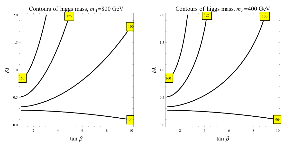
We show the contours of the lifted Higgs mass as a function of $\delta\lambda_{1}$ and $\tan\beta$ in Fig 1.

As we expect for a term involving only the up-type Higgs, the new quartic is more efficient at raising the light Higgs boson mass to 125 GeV in the limit of large $\tan\beta$. Furthermore, because the MSSM tree-level contribution is suppressed at small $\tan\beta$, it becomes even more difficult to obtain $\delta\lambda_{1}$ large enough in that case. This is illustrated by the contours of constant Higgs mass in the $\left(\tan\beta,\delta\lambda_{1}\right)$ plane in Figure 1.

To evaluate the tuning, we first take a derivative with respect to $M_{d}^{2}$. We use the fact that $b=m_{A}^{2}\sin\beta\cos\beta$ (a result that is unchanged from the MSSM case) and thus that $M_{d}^{2}$ can be written in terms of the physical parameters $m_{Z}^{2},m_{A}^{2},$ and $\tan\beta$ as $M_{d}^{2}=m_{A}^{2}\sin^{2}\beta-\frac{1}{2}m_{Z}^{2}\cos(2\beta)$. The resulting expression is:

This expression is not very enlightening on its own, but the main question we are interested in is: if we allow at most a given amount of fine-tuning, can we infer a bound on the physical masses of heavy particles? For this question, it is reasonable to expand the tuning measure at large $m_{A}^{2}$. We will also assume that the value of $\delta\lambda_{1}$ is chosen to fix the Higgs mass $m_{h}^{2}$ as in eq. (11). The result is:

From this we can see that if $m_{A}^{2}\gg m_{h}^{2}$, the theory becomes very fine-tuned unless $\sin(2\beta)$ is small, which happens in the $\tan\beta\gg 1$ limit. We explicitly illustrate this point in Fig. 2 where we plot the contours of fine tuning as a function of $m_{A}$ and $\tan\beta$. The precise value of $\delta\lambda_{1}$ on this plot is set by demanding $m_{h}=125$ GeV.

As expected, one gets very low fine tuning for very large values of $\tan\beta$. Even now the large $\tan\beta$ region can be partially explored by the LHC, due to a robust $H^{0},~A^{0}\to\tau^{+}\tau^{-}$ decay mode which can be directly probed. In Fig. 2 we show a green region, which has been directly excluded by the CMS search [44] for $H^{0}\to\tau^{+}\tau^{-}$. We anticipate that much more significant gains will be made by LHC14.

However, another important constraint on the large $\tan\beta$ region comes from the measurement of the flavor-violating decay $b\to s\gamma$, which we will explore in detail in Section 3. There we will find that, for very low-scale SUSY breaking (mediated at $\Lambda=10$ TeV), one can accommodate $\tan\beta\approx 30$ if one allows a factor of 10 tuning in the stop sector. (Indirect constraints from Higgs decays already force us to accept a minimum factor of about 5 tuning in the stop sector [36].) Using the formula above, we find that if we allow at most an additional factor of 10 tuning in EWSB, for a combined 1% tuning, we have $m_{A}\mathrel{\hbox to0.0pt{\lower 4.0pt\hbox{\hskip 1.0pt$\sim$}\hss}\raise 1.0pt\hbox{$<$}}8.4$ TeV. Probing such large values of $m_{A}$ will require future hadron colliders, more powerful than the LHC. On the other hand, we will find in Section 3.3 that with even a slightly higher mediation scale $\Lambda=30$ TeV the bound from $b\to s\gamma$ becomes notably stronger: $\tan\beta\mathrel{\hbox to0.0pt{\lower 4.0pt\hbox{\hskip 1.0pt$\sim$}\hss}\raise 1.0pt\hbox{$<$}}10$. In this case, allowing for at most an additional factor of 10 tuning in EWSB implies $m_{A}\mathrel{\hbox to0.0pt{\lower 4.0pt\hbox{\hskip 1.0pt$\sim$}\hss}\raise 1.0pt\hbox{$<$}}2.8$ TeV. If we view the factor of 10 tuning in the stop sector as already deviating from naturalness, and want to ask for no additional tuning in EWSB, we have the stronger condition $m_{A}\mathrel{\hbox to0.0pt{\lower 4.0pt\hbox{\hskip 1.0pt$\sim$}\hss}\raise 1.0pt\hbox{$<$}}0.9$ TeV. Furthermore, higher mediation scales only strengthen the $\tan\beta$ upper bound from $b\to s\gamma$, so although parts of the natural parameter space may require future colliders to probe, in much of the parameter space the heavy Higgs bosons should be accessible at the LHC. Measurements of the light Higgs boson decay modes at the 14 TeV LHC with 300 fb^-1 of data will probe the range of $m_{A}$ up to about 450 GeV [45]. Heavier masses can be probed only by direct searches or higher precision measurements at the high luminosity LHC or especially future $e^{+}e^{-}$ colliders.

This is the quartic extension that arises in the NMSSM or $\lambda$SUSY. It does not change the pseudoscalar mass relation $m_{A}^{2}=2b/\sin(2\beta)$. In this case, we find that the light Higgs mass is corrected as:

In this case moderate values of $\tan\beta$ are most effective for raising the Higgs mass, because the correction term involves $v_{d}$ and is suppressed in the large $\tan\beta$ limit. In fact, it is impossible to get $m_{h}=125$ GeV with large $\tan\beta$. On top of that, we often need large, almost non-perturbative values of $\delta\lambda_{5}$ in order to get the correct value of the SM-like Higgs mass.

The tuning measure in this case is:

Again, this expression simplifies in the limit $m_{A}^{2}\gg m_{h}^{2},m_{Z}^{2}$, choosing $\delta\lambda_{5}$ to fix the Higgs mass $m_{h}^{2}$ as in eq. (14):

This suggests that $\lambda_{5}$ extension is typically fine tuned, since it is not easy to find a perturbative $\delta\lambda_{5}$ for a light pseudo-scalar $A$. We show this point explicitly in Fig 4. Most of the solutions for $\delta\lambda_{5}$ are already fine tuned, and those which are technically not fine tuned require very large values of $\delta\lambda_{5}$. The region with order-one values of $\delta\lambda_{5}$ and low fine-tuning has $m_{A}\mathrel{\hbox to0.0pt{\lower 4.0pt\hbox{\hskip 1.0pt$\sim$}\hss}\raise 1.0pt\hbox{$<$}}1$ TeV, so the heavy Higgs bosons may be accessible at the LHC.

The simplest estimate for the smallest natural choice of $A_{t}$, assuming running from a relatively low scale $\Lambda$, is

If we run from a higher scale, we can do a somewhat more careful estimate by resumming large logarithms.

What we have called $A_{t}$ is really $a_{t}/y_{t}$, where $a_{t}$ is the coefficient of the three-scalar operator in the Lagrangian. Keeping only the one-loop terms involving $g_{3}$ or $y_{t}$, the RG evolution of $a_{t}$ is related to that of the gluino mass by the equation (e.g. [71])

If we assume that $a_{t}\approx 0$ at some mediation scale $M_{\rm med}$ (as is true in a number of models, including gauge mediation), we can use this equation together with the RGEs for $g_{3},y_{t},$ and $M_{3}$ to plot the low-scale value of $A_{t}$ as a function of the low-scale gluino mass parameter $M_{3}$ and the mediation scale. We show this in Fig. 6.

What we learn from this is that typically, the RG contribution to $A_{t}$ ranges from $-200~{\rm GeV}$ to $-750~{\rm GeV}$ over a wide range of mediation scales and for gluinos near 1 TeV. Thus, a smaller trilinear coupling $A_{t}$ will generally imply some tuning of a positive tree-level value at the mediation scale against a negative loop correction from gluinos. (Here we use “tree-level” loosely for the value of $A_{t}$ at the mediation scale; in a given model, it may arise from loops, but we distinguish it from the contribution generated in the RGE.) We will quantify this tuning in an intuitive way. Given that $A_{t}$ is a sum $A_{t}=A_{t}^{\rm tree}+A_{t}^{\rm loop}$, we can measure a tuning by the amount of cancelation:

In the regime where the two terms nearly cancel, this behaves similarly to other tuning measures like that of Barbieri and Giudice [1]. If there is no significant cancelation (e.g. if $A_{t}$ at the mediation scale is much larger than the gluino-generated term), it asymptotes to $1$. This is a desirable property for a tuning measure to have, because we would like to be able to compute a combined tuning in multiple variables as a product of independent tunings in each variable.

As $\tan\beta$ increases, the Yukawa couplings needed to generate the $b$ and $\tau$ masses from the VEV of $H_{d}$ become large. However, a new source of masses arises from loop effects that generate the “wrong-Higgs” Yukawa couplings $H_{u}^{\dagger}Qd^{c}$ and $H_{u}^{\dagger}Le^{c}$. For sufficiently large $\tan\beta$ we can think of the $b$ and $\tau$ masses as arising entirely for these effects, in what has been called the uplifted supersymmetric Higgs region of parameter space [72, 73]. In this part of parameter space, we must exercise some caution in our argument about the size of the $b\to s\gamma$ amplitude. The same loop diagram that generates the wrong-Higgs bottom quark Yukawa coupling also generates $b\to s\gamma$, when one external $b$ quark is replaced by a strange quark and a photon is attached to an internal line. (Compare the loops generating Yukawas in Fig. 7 to those for $b\to s\gamma$ in Fig. 5.) As a result, $b\to s\gamma$ is no longer enhanced by a factor of $\tan\beta$ relative to the $b$-quark mass, and we should be concerned that data on $b\to s\gamma$ can’t actually rule out very large values of $\tan\beta$.

This concern is conceptually reasonable but proves to be numerically unfounded. The uplifted region of parameter space lies at very large values of $\tan\beta$ and also requires large values of $\mu$, putting it outside of what we consider to be natural SUSY parameter space. In all of our computations, we will use the formulas of Ref. [68], in which the corrections to the $b\to s\gamma$ amplitude are proportional to $\tan\beta/(1+\epsilon_{b}\tan\beta)$, where $\epsilon_{b}$ in the denominator is a loop factor correcting for the wrong-Higgs contribution to the $b$-quark mass. The statement that the uplifted regime does not change our conclusion is that $\epsilon_{b}\tan\beta$ is at most ${\cal O}(1)$ for reasonable input parameters, whereas removing the bound at large $\tan\beta$ would require that it be $\gg 1$.

It is easy to see that naturalness is in tension with the uplifted regime by inspection of the loop corrections. The approximate result for $\epsilon_{b}$ in the limit $m_{Q_{3}}^{2}=m_{u^{c}_{3}}^{2}=m_{d^{c}_{3}}^{2}\equiv m_{\tilde{q}}^{2}$ assuming $M_{3}^{2}\gg m_{\tilde{q}}^{2}\gg\mu^{2}$ is

Numerically, we expect the gluino loop contribution to $\epsilon_{b}$, which is $\sim\mu/M_{3}$, to dominate in most of the natural SUSY parameter space. Note that for naturalness, we prefer $\mu$ as small as possible (close to 100 GeV), whereas experimentally we know that $M_{3}\mathrel{\hbox to0.0pt{\lower 4.0pt\hbox{\hskip 1.0pt$\sim$}\hss}\raise 1.0pt\hbox{$>$}}1~{\rm TeV}$. Furthermore, the gluino loop drags the stop and sbottom soft masses up, so the log is rarely large. Estimating $\mu/M_{3}\mathrel{\hbox to0.0pt{\lower 4.0pt\hbox{\hskip 1.0pt$\sim$}\hss}\raise 1.0pt\hbox{$<$}}0.2$ and $\log(M_{3}^{2}/m_{\tilde{q}}^{2})\mathrel{\hbox to0.0pt{\lower 4.0pt\hbox{\hskip 1.0pt$\sim$}\hss}\raise 1.0pt\hbox{$<$}}3$, we see that $\epsilon_{b}\mathrel{\hbox to0.0pt{\lower 4.0pt\hbox{\hskip 1.0pt$\sim$}\hss}\raise 1.0pt\hbox{$<$}}10^{-2}$, so that $\epsilon_{b}\tan\beta$ becomes an order-one number only at $\tan\beta\sim 100$. One could try to get around this conclusion by choosing very large values of $A_{t}$ to enhance the second term, but this is not very well-motivated and potentially runs into problems with vacuum stability [74]. Increasing the first term requires going to large $\mu$ and thus indicates significant tree-level tuning for electroweak symmetry breaking. In short, the uplifted regime is of little relevance for a study of natural SUSY, and will not interfere with our inference of a bound on $\tan\beta$ from $b\to s\gamma$ and naturalness.

For the experimental bound on $b\to s\gamma$, we will follow Ref. [68] in taking the SM prediction to be [75] ${\rm Br}(B\to X_{s}\gamma)_{\rm SM}=\left(3.15\pm 0.23\right)\times 10^{-4}$ and the experimental value to be [76, 77] ${\rm Br}(B\to X_{s}\gamma)_{\rm exp}=\left(3.43\pm 0.22\right)\times 10^{-4}$. Given these values, we estimate that at 95% confidence level the ratio $R_{bs\gamma}$ of the true value of the branching ratio to its Standard Model value lies in the range

Because the data prefer a slightly high value relative to the Standard Model, constraints are weaker on the scenario where new physics constructively interferes with the SM amplitude. This happens when $\mu A_{t}>0$. Because small $A_{t}$ is easiest to achieve if the RG contribution from the gluino dominates, this corresponds to a negative sign for $\mu M_{3}$. The case $\mu A_{t}<0$, arising if $\mu$ and the gluino mass term have the same sign, is more strongly constrained.

We have plotted the largest allowed value of $\tan\beta$, with various naturalness constraints superimposed, in Fig. 8. In this figure $\mu$ is fixed to 100 GeV. We have also fixed $\left|M_{3}\right|=1.3$ TeV, $m_{d_{3}}=2$ TeV, $M_{2}=0.5$ TeV, and $\zeta$ (a parameter defined in ref. [68] related to the relative size of various MFV terms in the soft mass matrices) equal to 0.5. We assume that running begins at $\Lambda=10$ TeV, a fairly extreme limit of low-scale SUSY breaking, in order to be conservative about tuning measures. Bounds on $\tan\beta$ become stronger if $\mu$ increases. The plot is relatively insensitive to the other parameters, but we have included them for concreteness. We have checked that including the stop–chargino loop alone, with all other superpartners decoupled, makes very little difference in the result. We plot two cases with two different signs of $M_{3}$ (relative to $\mu$). The sign of $M_{3}$ determines the sign of $A_{t}^{\rm loop}$ which enters in the tuning measure Eq. (21).

The naturalness constraints are defined in terms of two tunings. First, large stop soft masses correspond to a tuning of the up-type Higgs soft mass parameter, which is quantified by [5, 6]

The second tuning arises for small values of $A_{t}$, as quantified in the expression $\Delta_{A_{t}}$ of Eq. (21). In Fig. 8, regions of large $\Delta_{\tilde{t}}$ are shaded red and regions of large $\Delta_{A_{t}}$ are shaded purple. One can see that large values of $\tan\beta$ are allowed only if $A_{t}$ is small or the stop masses are large, indicating that at least one of these tuning measures is becoming large. For instance, there are two corners of parameter space where $\Delta_{A_{t}}=\Delta_{\tilde{t}}=5$, one at negative $A_{t}$ and one at positive $A_{t}$ (where the sign is understood relative to that of $\mu$). In the case $M_{3}<0$, at the former point, the largest 95% CL allowed value of $\tan\beta$ is less than 10; at the latter, it is about 25. Thus, as noted above, the case of positive $A_{t}$ is less strongly constrained.

We have no particular reason to think that cancellations in $m_{H_{u}}^{2}$ and in $A_{t}$ will happen at the same point in parameter space, although perhaps one could imagine a model in which this is true. If the tunings are independent, we can think of an overall tuning $\Delta=\Delta_{\tilde{t}}\Delta_{A_{t}}$ which is simply the product of the two individual tunings. In other words, if we have to adjust two unrelated parameters to the 10% level, this may reasonably be thought of as a 1% tuning in parameter space. With such independent tunings in mind, we have plotted dashed black contours in Fig. 8 that show where $\Delta=10$. We see that the combined tuning is mildest whenever $M_{3}A_{t}<0$, which is driven by the fact that $\Delta_{A_{t}}$ prefers $A_{t}$ to be either near its loop-generated value or much bigger.

The most optimistic region of parameter space has $\mu A_{t}>0$ (so that the new physics contribution constructively interferes with the SM and improves agreement with data) and $A_{t}M_{3}<0$ (so that the trilinear can be mostly generated from the RG). From the figure, we can see that this marginally allows $\tan\beta\approx 28$ with a combined tuning $\Delta\approx 10$ coming almost entirely from the stop mass $m_{\tilde{t}}\approx 600~{\rm GeV}$. The plots make it clear that allowing $\tan\beta>30$ will require either quite heavy stops—out of the range that can be considered truly natural—or a cancelation in $A_{t}$, or both. We think that it is very conservative to conclude that generic natural SUSY requires $\tan\beta<30$.

In fact, we are usually understating the required cancelation in $A_{t}$, because most reasonable models will run from a higher UV scale and generate values of $A_{t}$ a factor of 2 or more larger than we have considered. Even a slightly larger amount of running produces a significantly stronger conclusion, as we illustrate in Fig. 9. Beginning the RGE at 30 TeV instead of 10 TeV produces a larger value of $A_{t}^{\rm loop}$ and also increases the stop-generated contribution to $m_{H_{u}}^{2}$. In this case, the conclusion is already that $\tan\beta<10$. We show how the bound on $\tan\beta$ changes with the mediation scale in the lower panel of Fig. 9. Running from 100 TeV already requires $\tan\beta<3.4$ for consistency with an overall tuning $\Delta<10$. (In fact, the bound already hits $\tan\beta=1$ when the mediation scale $\Lambda\approx 350$ TeV, indicating that models of high-scale SUSY breaking will require significant fine-tuning for compatibility with the $b\to s\gamma$ measurement.) Although the choice of a tuning measure is to some extent a matter of taste, it is clear that accommodating $\tan\beta\mathrel{\hbox to0.0pt{\lower 4.0pt\hbox{\hskip 1.0pt$\sim$}\hss}\raise 1.0pt\hbox{$>$}}10$ requires both very low-scale mediation and a mild tuning. We also show, with the dashed orange line in the lower panel of Fig. 9, that allowing for more tuning significantly increases the range of allowed $\tan\beta$. If we allow $\Delta=30$ rather than 10, we can accommodate $\tan\beta=30$ even with running from 100 TeV, and $\tan\beta=10$ even with running from 1000 TeV. Still, high-scale SUSY breaking is highly constrained even allowing for this larger amount of tuning.

As a simpler estimate, we can use the one loop RG approximation eq. (19) for $A_{t}^{\rm loop}$, write the average stop mass in terms of the tuning $\Delta_{\tilde{t}}$ from eq. (24), and use the leading term in equation (18) to estimate that

implying

This is a useful check that the more detailed numerical results are reasonable. The $\left(\log\Lambda\right)^{-3}$ behavior explains the rapid improvement of the bound as we increase $\Lambda$ above 10 TeV that we saw in Fig. 9.

This very rare process is often quoted as the best possible constraint on SUSY with large $\tan\beta$. Indeed the most important SUSY contribution to $B_{s}\to\mu^{+}\mu^{-}$ is proportional to $\tan^{3}\beta$ [78, 79], and therefore is naively expected to be very sensitive to natural SUSY. However we find that all the constraints that we get from this process are subdominant to $b\to s\gamma$ constraints. There is a simple explanation for why this happens. Although the matrix element is enhanced by $\tan^{3}\beta$, it is also suppressed by $m_{A}^{2}$. As we have learned in Sec. 2, in the large $\tan\beta$ limit the fine tuning of EWSB stays approximately constant along the contours of $m_{A}\tan\beta=const$. Therefore, effectively the matrix element is enhanced only by a single power of $\tan\beta$, precisely as is $b\to s\gamma$.

On the other hand, the rate of $B_{s}\to\mu^{+}\mu^{-}$ is measured to much worse precision than $b\to s\gamma$. While the process $b\to s\gamma$ is measured to the precision of better than 10%, Ref. [80] gives the following 95% CL bound on $B_{s}\to\mu^{+}\mu^{-}$:

Based on the SM prediction [81]

from these equations we estimate that at 95% confidence level

The lower bound is meaningless in large $\tan\beta$ regime: in SUSY one cannot get $R_{B_{s}\to\mu^{+}\mu^{-}}$ smaller than 0.5, unless the SUSY contribution is dominated by the $Z$-penguin.³³ 3 The reason for this is that there is a contribution with $H^{0}$ exchange that interferes destructively with the Standard Model, and a contribution with $A^{0}$ exchange that does not interfere and is equal to the $H^{0}$ amplitude to the extent that $m_{A}\approx m_{H^{0}}$. Thus the squared matrix element goes as $\left|A_{\rm SM}-A_{\rm NP}\right|^{2}+\left|A_{\rm NP}\right|^{2}\geq\frac{1}{2}\left|A_{\rm SM}\right|^{2}$. If the $Z$ penguin contribution matters, this argument is no longer strictly true. But the $Z$ penguin goes only as $\tan^{2}\beta$ and is suppressed by the mass insertion $\delta_{LR}$ in the up sector (see [82] for relevant expressions), so is generally expected to be less important. On the other hand the upper bound is weak, allowing ${\cal O}(1)$ deviations from the SM-predicted values. Therefore the bounds on $\tan\beta$ one gets from this process are much weaker than those one gets from $b\to s\gamma$. To illustrate these points we show these bounds, considering (as in the $b\to s\gamma$ example) only the higgsino loop contribution, in Fig. 10, showing the maximal allowed values of $\tan\beta$ for $m_{A}=400$ GeV. We see that these constraints are very clearly subdominant to the $b\to s\gamma$ constraints in Fig. 8. At higher $m_{A}$ these constraints quickly decouple.

If the gluino has a Dirac mass rather than the standard Majorana mass, our argument breaks down because $A_{t}$ can naturally be smaller, protected by $R$-symmetry. Supersymmetry with Dirac gauginos has received a great deal of recent attention: see (for example) refs. [83, 84, 85, 86, 87, 8, 88, 89, 90, 91, 92, 93, 94]. An $R$-symmetry forbids a $\mu$-term as the higgsino mass, so these models typically involve new doublets that pair with the usual Higgs doublets to form massive higgsinos. The $A$-term is also forbidden. Depending on how and to what extent the $R$-symmetry is broken, a remnant of our argument may survive in these models. For the most part, however, we expect that these models evade our argument and that a detailed look at the EWSB conditions and naturalness in these theories will require a completely different perspective. Some aspects of naturalness in such theories have been addressed in refs. [91, 92, 94]. Although this loophole exists, models with Dirac gauginos are necessarily more baroque than traditional SUSY models, and we do not feel that they undermine the motivation for viewing heavy Higgs bosons as key channels in which to search for naturalness.

References

- [1] R. Barbieri and G. Giudice, “Upper Bounds on Supersymmetric Particle Masses,” Nucl.Phys. B306 (1988) 63.
- [2] S. Dimopoulos and G. Giudice, “Naturalness constraints in supersymmetric theories with nonuniversal soft terms,” Phys.Lett. B357 (1995) 573–578, arXiv:hep-ph/9507282 [hep-ph].
- [3] A. Pomarol and D. Tommasini, “Horizontal symmetries for the supersymmetric flavor problem,” Nucl.Phys. B466 (1996) 3–24, arXiv:hep-ph/9507462 [hep-ph].
- [4] A. G. Cohen, D. Kaplan, and A. Nelson, “The More minimal supersymmetric standard model,” Phys.Lett. B388 (1996) 588–598, arXiv:hep-ph/9607394 [hep-ph].
- [5] R. Kitano and Y. Nomura, “Supersymmetry, naturalness, and signatures at the LHC,” Phys.Rev. D73 (2006) 095004, arXiv:hep-ph/0602096 [hep-ph].
- [6] M. Perelstein and C. Spethmann, “A Collider signature of the supersymmetric golden region,” JHEP 0704 (2007) 070, arXiv:hep-ph/0702038 [hep-ph].
- [7] M. Papucci, J. T. Ruderman, and A. Weiler, “Natural SUSY Endures,” JHEP 1209 (2012) 035, arXiv:1110.6926 [hep-ph].
- [8] C. Brust, A. Katz, S. Lawrence, and R. Sundrum, “SUSY, the Third Generation and the LHC,” JHEP 1203 (2012) 103, arXiv:1110.6670 [hep-ph].
- [9] H. Baer, V. Barger, and D. Mickelson, “How conventional measures overestimate electroweak fine-tuning in supersymmetric theory,” Phys.Rev. D88 (2013) 095013, arXiv:1309.2984 [hep-ph].
- [10] P. Meade and M. Reece, “Top partners at the LHC: Spin and mass measurement,” Phys.Rev. D74 (2006) 015010, arXiv:hep-ph/0601124 [hep-ph].
- [11] M. Farina, M. Perelstein, and N. R.-L. Lorier, “Higgs Couplings and Naturalness,” arXiv:1305.6068 [hep-ph].
- [12] G. D. Kribs, A. Martin, and A. Menon, “Natural Supersymmetry and Implications for Higgs physics,” Phys.Rev. D88 (2013) 035025, arXiv:1305.1313 [hep-ph].
- [13] K. Kowalska and E. M. Sessolo, “Natural MSSM after the LHC 8 TeV run,” Phys.Rev. D88 (2013) 075001, arXiv:1307.5790 [hep-ph].
- [14] C. Han, K.-I. Hikasa, L. Wu, J. M. Yang, and Y. Zhang, “Current experimental bounds on stop mass in natural SUSY,” JHEP 1310 (2013) 216, arXiv:1308.5307 [hep-ph].
- [15] N. Craig, “The State of Supersymmetry after Run I of the LHC,” arXiv:1309.0528 [hep-ph].
- [16] J. L. Feng, “Naturalness and the Status of Supersymmetry,” Ann.Rev.Nucl.Part.Sci. 63 (2013) 351–382, arXiv:1302.6587 [hep-ph].
- [17] E. Hardy, “Is Natural SUSY Natural?,” JHEP 1310 (2013) 133, arXiv:1306.1534 [hep-ph].
- [18] P. Batra, A. Delgado, D. E. Kaplan, and T. M. Tait, “The Higgs mass bound in gauge extensions of the minimal supersymmetric standard model,” JHEP 0402 (2004) 043, arXiv:hep-ph/0309149 [hep-ph].
- [19] R. Barbieri, L. J. Hall, Y. Nomura, and V. S. Rychkov, “Supersymmetry without a Light Higgs Boson,” Phys.Rev. D75 (2007) 035007, arXiv:hep-ph/0607332 [hep-ph].
- [20] M. Dine, N. Seiberg, and S. Thomas, “Higgs physics as a window beyond the MSSM (BMSSM),” Phys.Rev. D76 (2007) 095004, arXiv:0707.0005 [hep-ph].
- [21] L. J. Hall, D. Pinner, and J. T. Ruderman, “A Natural SUSY Higgs Near 126 GeV,” JHEP 1204 (2012) 131, arXiv:1112.2703 [hep-ph].
- [22] T. Gherghetta, B. von Harling, A. D. Medina, and M. A. Schmidt, “The price of being SM-like in SUSY,” JHEP 1404 (2014) 180, arXiv:1401.8291 [hep-ph].
- [23] K. Ishiwata, N. Nagata, and N. Yokozaki, “Natural Supersymmetry and constraints,” Phys.Lett. B710 (2012) 145–148, arXiv:1112.1944 [hep-ph].
- [24] J. F. Gunion and H. E. Haber, “The CP conserving two Higgs doublet model: The Approach to the decoupling limit,” Phys.Rev. D67 (2003) 075019, arXiv:hep-ph/0207010 [hep-ph].
- [25] L. Randall, “Two Higgs Models for Large Tan Beta and Heavy Second Higgs,” JHEP 0802 (2008) 084, arXiv:0711.4360 [hep-ph].
- [26] K. Blum and R. T. D’Agnolo, “2 Higgs or not 2 Higgs,” Phys.Lett. B714 (2012) 66–69, arXiv:1202.2364 [hep-ph].
- [27] X. Lu, H. Murayama, J. T. Ruderman, and K. Tobioka, “A Natural Higgs Mass in Supersymmetry from Non-Decoupling Effects,” Phys.Rev.Lett. 112 (2014) 191803, arXiv:1308.0792 [hep-ph].
- [28] A. Maloney, A. Pierce, and J. G. Wacker, “D-terms, unification, and the Higgs mass,” JHEP 0606 (2006) 034, arXiv:hep-ph/0409127 [hep-ph].
- [29] C. Cheung and H. L. Roberts, “Higgs Mass from D-Terms: a Litmus Test,” JHEP 1312 (2013) 018, arXiv:1207.0234 [hep-ph].
- [30] J. Espinosa and M. Quiros, “On Higgs boson masses in nonminimal supersymmetric standard models,” Phys.Lett. B279 (1992) 92–97.
- [31] K. Agashe, Y. Cui, and R. Franceschini, “Natural Islands for a 125 GeV Higgs in the scale-invariant NMSSM,” JHEP 1302 (2013) 031, arXiv:1209.2115 [hep-ph].
- [32] T. Gherghetta, B. von Harling, A. D. Medina, and M. A. Schmidt, “The Scale-Invariant NMSSM and the 126 GeV Higgs Boson,” JHEP 02 (2013) 032, arXiv:1212.5243 [hep-ph].
- [33] K. Agashe, A. Azatov, A. Katz, and D. Kim, “Improving the tunings of the MSSM by adding triplets and singlet,” Phys.Rev. D84 (2011) 115024, arXiv:1109.2842 [hep-ph].
- [34] H. Baer, V. Barger, D. Mickelson, and M. Padeffke-Kirkland, “SUSY models under siege: LHC constraints and electroweak fine-tuning,” arXiv:1404.2277 [hep-ph].
- [35] S. Fichet, “Quantified naturalness from Bayesian statistics,” Phys.Rev. D86 (2012) 125029, arXiv:1204.4940 [hep-ph].
- [36] J. Fan and M. Reece, “A New Look at Higgs Constraints on Stops,” arXiv:1401.7671 [hep-ph].
- [37] H. E. Haber and R. Hempfling, “Can the mass of the lightest Higgs boson of the minimal supersymmetric model be larger than m(Z)?,” Phys.Rev.Lett. 66 (1991) 1815–1818.
- [38] R. Barbieri, M. Frigeni, and F. Caravaglios, “The Supersymmetric Higgs for heavy superpartners,” Phys.Lett. B258 (1991) 167–170.
- [39] J. Casas, J. Espinosa, M. Quiros, and A. Riotto, “The Lightest Higgs boson mass in the minimal supersymmetric standard model,” Nucl.Phys. B436 (1995) 3–29, arXiv:hep-ph/9407389 [hep-ph].
- [40] M. S. Carena, J. Espinosa, M. Quiros, and C. Wagner, “Analytical expressions for radiatively corrected Higgs masses and couplings in the MSSM,” Phys.Lett. B355 (1995) 209–221, arXiv:hep-ph/9504316 [hep-ph].
- [41] N. Craig, D. Green, and A. Katz, “(De)Constructing a Natural and Flavorful Supersymmetric Standard Model,” JHEP 1107 (2011) 045, arXiv:1103.3708 [hep-ph].
- [42] N. Craig and A. Katz, “A Supersymmetric Higgs Sector with Chiral D-terms,” JHEP 1305 (2013) 015, arXiv:1212.2635 [hep-ph].
- [43] A. Bharucha, A. Goudelis, and M. McGarrie, “En-gauging Naturalness,” arXiv:1310.4500 [hep-ph].
- [44] CMS Collaboration, “Higgs to tau tau (MSSM),” Tech. Rep. CMS-PAS-HIG-13-021, CERN, Geneva, 2013. http://cds.cern.ch/record/1623367.
- [45] R. S. Gupta, M. Montull, and F. Riva, “SUSY Faces its Higgs Couplings,” JHEP 1304 (2013) 132, arXiv:1212.5240 [hep-ph].
- [46] K. Blum, R. T. D’Agnolo, and J. Fan, “Natural SUSY Predicts: Higgs Couplings,” JHEP 1301 (2013) 057, arXiv:1206.5303 [hep-ph].
- [47] J. R. Espinosa, C. Grojean, V. Sanz, and M. Trott, “NSUSY fits,” JHEP 1212 (2012) 077, arXiv:1207.7355 [hep-ph].
- [48] N. Oshimo, “Radiative meson decay in supersymmetric models,” Nucl.Phys. B404 (1993) 20–41.
- [49] R. Barbieri and G. Giudice, “ decay and supersymmetry,” Phys.Lett. B309 (1993) 86–90, arXiv:hep-ph/9303270 [hep-ph].
- [50] Y. Okada, “Light stop and the process,” Phys.Lett. B315 (1993) 119–123, arXiv:hep-ph/9307249 [hep-ph].
- [51] R. Garisto and J. Ng, “Supersymmetric with large chargino contributions,” Phys.Lett. B315 (1993) 372–378, arXiv:hep-ph/9307301 [hep-ph].
- [52] H. Baer, M. Brhlik, D. Castano, and X. Tata, “ constraints on the minimal supergravity model with large tan Beta,” Phys.Rev. D58 (1998) 015007, arXiv:hep-ph/9712305 [hep-ph].
- [53] G. Degrassi, P. Gambino, and G. Giudice, “ in supersymmetry: Large contributions beyond the leading order,” JHEP 0012 (2000) 009, arXiv:hep-ph/0009337 [hep-ph].
- [54] M. S. Carena, D. Garcia, U. Nierste, and C. E. Wagner, “ and supersymmetry with large tan ,” Phys.Lett. B499 (2001) 141–146, arXiv:hep-ph/0010003 [hep-ph].
- [55] ALEPH Collaboration, A. Heister et al., “Search for charginos nearly mass degenerate with the lightest neutralino in e+ e- collisions at center-of-mass energies up to 209-GeV,” Phys.Lett. B533 (2002) 223–236, arXiv:hep-ex/0203020 [hep-ex].
- [56] DELPHI Collaboration, J. Abdallah et al., “Searches for supersymmetric particles in collisions up to 208-GeV and interpretation of the results within the MSSM,” Eur.Phys.J. C31 (2003) 421–479, arXiv:hep-ex/0311019 [hep-ex].
- [57] OPAL Collaboration, G. Abbiendi et al., “Search for nearly mass degenerate charginos and neutralinos at LEP,” Eur.Phys.J. C29 (2003) 479–489, arXiv:hep-ex/0210043 [hep-ex].
- [58] L3 Collaboration, M. Acciarri et al., “Search for charginos with a small mass difference with the lightest supersymmetric particle at = 189 GeV,” Phys.Lett. B482 (2000) 31–42, arXiv:hep-ex/0002043 [hep-ex].
- [59] S. Gori, S. Jung, and L.-T. Wang, “Cornering electroweakinos at the LHC,” JHEP 1310 (2013) 191, arXiv:1307.5952 [hep-ph].
- [60] C. Han, A. Kobakhidze, N. Liu, A. Saavedra, L. Wu, and J. M. Yang, “Probing Light Higgsinos in Natural SUSY from Monojet Signals at the LHC,” JHEP 1402 (2014) 049, arXiv:1310.4274 [hep-ph].
- [61] P. Schwaller and J. Zurita, “Compressed electroweakino spectra at the LHC,” JHEP 1403 (2014) 060, arXiv:1312.7350 [hep-ph].
- [62] Z. Han, G. D. Kribs, A. Martin, and A. Menon, “Hunting Quasi-Degenerate Higgsinos,” Phys.Rev. D89 (2014) 075007, arXiv:1401.1235 [hep-ph].
- [63] ATLAS Collaboration, G. Aad et al., “Search for new phenomena in final states with large jet multiplicities and missing transverse momentum at TeV proton-proton collisions using the ATLAS experiment,” JHEP 1310 (2013) 130, arXiv:1308.1841 [hep-ex].
- [64] CMS Collaboration, S. Chatrchyan et al., “Search for supersymmetry in pp collisions at = 8 TeV in events with a single lepton, large jet multiplicity, and multiple b jets,” arXiv:1311.4937 [hep-ex].
- [65] CMS Collaboration, S. Chatrchyan et al., “Search for new physics in the multijet and missing transverse momentum final state in proton-proton collisions at = 8 TeV,” arXiv:1402.4770 [hep-ex].
- [66] ATLAS Collaboration, “Search for massive particles in multijet signatures with the ATLAS detector in TeV pp collisions at the LHC,”. http://cds.cern.ch/record/1595753.
- [67] J. A. Evans, Y. Kats, D. Shih, and M. J. Strassler, “Toward Full LHC Coverage of Natural Supersymmetry,” arXiv:1310.5758 [hep-ph].
- [68] W. Altmannshofer, M. Carena, N. R. Shah, and F. Yu, “Indirect Probes of the MSSM after the Higgs Discovery,” JHEP 1301 (2013) 160, arXiv:1211.1976 [hep-ph].
- [69] A. Freitas and U. Haisch, “ gamma in two universal extra dimensions,” Phys.Rev. D77 (2008) 093008, arXiv:0801.4346 [hep-ph].
- [70] F. Mescia and J. Virto, “Natural SUSY and Kaon Mixing in view of recent results from Lattice QCD,” Phys.Rev. D86 (2012) 095004, arXiv:1208.0534 [hep-ph].
- [71] S. P. Martin, “A Supersymmetry primer,” arXiv:hep-ph/9709356 [hep-ph].
- [72] B. A. Dobrescu and P. J. Fox, “Uplifted supersymmetric Higgs region,” Eur.Phys.J. C70 (2010) 263–270, arXiv:1001.3147 [hep-ph].
- [73] W. Altmannshofer and D. M. Straub, “Viability of MSSM scenarios at very large tan(beta),” JHEP 1009 (2010) 078, arXiv:1004.1993 [hep-ph].
- [74] A. Kusenko, P. Langacker, and G. Segre, “Phase transitions and vacuum tunneling into charge and color breaking minima in the MSSM,” Phys.Rev. D54 (1996) 5824–5834, arXiv:hep-ph/9602414 [hep-ph].
- [75] M. Misiak, H. Asatrian, K. Bieri, M. Czakon, A. Czarnecki, et al., “Estimate of Br at O(),” Phys.Rev.Lett. 98 (2007) 022002, arXiv:hep-ph/0609232 [hep-ph].
- [76] BaBar Collaboration, J. Lees et al., “Measurement of B(), the photon energy spectrum, and the direct CP asymmetry in decays,” Phys.Rev. D86 (2012) 112008, arXiv:1207.5772 [hep-ex].
- [77] Heavy Flavor Averaging Group Collaboration, Y. Amhis et al., “Averages of B-Hadron, C-Hadron, and tau-lepton properties as of early 2012,” arXiv:1207.1158 [hep-ex].
- [78] K. Babu and C. F. Kolda, “Higgs mediated in minimal supersymmetry,” Phys.Rev.Lett. 84 (2000) 228–231, arXiv:hep-ph/9909476 [hep-ph].
- [79] G. Isidori and A. Retico, “Scalar flavor changing neutral currents in the large tan beta limit,” JHEP 0111 (2001) 001, arXiv:hep-ph/0110121 [hep-ph].
- [80] LHCb Collaboration, R. Aaij et al., “First Evidence for the Decay ,” Phys.Rev.Lett. 110 (2013) 021801, arXiv:1211.2674 [hep-ex].
- [81] A. J. Buras, J. Girrbach, D. Guadagnoli, and G. Isidori, “On the Standard Model prediction for ,” Eur.Phys.J. C72 (2012) 2172, arXiv:1208.0934 [hep-ph].
- [82] P. H. Chankowski and L. Slawianowska, “ decay in the MSSM,” Phys.Rev. D63 (2001) 054012, arXiv:hep-ph/0008046 [hep-ph].
- [83] P. J. Fox, A. E. Nelson, and N. Weiner, “Dirac gaugino masses and supersoft supersymmetry breaking,” JHEP 0208 (2002) 035, arXiv:hep-ph/0206096 [hep-ph].
- [84] A. E. Nelson, N. Rius, V. Sanz, and M. Unsal, “The Minimal supersymmetric model without a mu term,” JHEP 0208 (2002) 039, arXiv:hep-ph/0206102 [hep-ph].
- [85] G. D. Kribs, E. Poppitz, and N. Weiner, “Flavor in supersymmetry with an extended R-symmetry,” Phys.Rev. D78 (2008) 055010, arXiv:0712.2039 [hep-ph].
- [86] R. Davies, J. March-Russell, and M. McCullough, “A Supersymmetric One Higgs Doublet Model,” JHEP 1104 (2011) 108, arXiv:1103.1647 [hep-ph].
- [87] C. Frugiuele and T. Gregoire, “Making the Sneutrino a Higgs with a Lepton Number,” Phys.Rev. D85 (2012) 015016, arXiv:1107.4634 [hep-ph].
- [88] G. D. Kribs and A. Martin, “Supersoft Supersymmetry is Super-Safe,” Phys.Rev. D85 (2012) 115014, arXiv:1203.4821 [hep-ph].
- [89] K. Benakli, M. D. Goodsell, and F. Staub, “Dirac Gauginos and the 125 GeV Higgs,” JHEP 1306 (2013) 073, arXiv:1211.0552 [hep-ph].
- [90] Z. Han, A. Katz, M. Son, and B. Tweedie, “Boosting Searches for Natural SUSY with RPV via Gluino Cascades,” Phys.Rev. D87 (2013) 075003, arXiv:1211.4025 [hep-ph].
- [91] A. Arvanitaki, M. Baryakhtar, X. Huang, K. van Tilburg, and G. Villadoro, “The Last Vestiges of Naturalness,” JHEP 1403 (2014) 022, arXiv:1309.3568 [hep-ph].
- [92] C. Csaki, J. Goodman, R. Pavesi, and Y. Shirman, “The Problem of Dirac Gauginos and its Solutions,” Phys.Rev. D89 (2014) 055005, arXiv:1310.4504 [hep-ph].
- [93] G. D. Kribs and N. Raj, “Mixed Gauginos Sending Mixed Messages to the LHC,” Phys.Rev. D89 (2014) 055011, arXiv:1307.7197 [hep-ph].
- [94] E. Bertuzzo, C. Frugiuele, T. Gregoire, and E. Ponton, “Dirac gauginos, R symmetry and the 125 GeV Higgs,” arXiv:1402.5432 [hep-ph].
- [95] A. Arbey, M. Battaglia, and F. Mahmoudi, “Supersymmetric Heavy Higgs Bosons at the LHC,” Phys.Rev. D88 (2013) 015007, arXiv:1303.7450 [hep-ph].
- [96] E. Brownson, N. Craig, U. Heintz, G. Kukartsev, M. Narain, et al., “Heavy Higgs Scalars at Future Hadron Colliders (A Snowmass Whitepaper),” arXiv:1308.6334 [hep-ex].
- [97] M. Carena, S. Heinemeyer, O. Stål, C. Wagner, and G. Weiglein, “MSSM Higgs Boson Searches at the LHC: Benchmark Scenarios after the Discovery of a Higgs-like Particle,” Eur. Phys. J. C73 (2013) 2552, arXiv:1302.7033 [hep-ph].
- [98] N. Craig, J. Galloway, and S. Thomas, “Searching for Signs of the Second Higgs Doublet,” arXiv:1305.2424 [hep-ph].
- [99] N. Craig, J. A. Evans, R. Gray, C. Kilic, M. Park, et al., “Multi-Lepton Signals of Multiple Higgs Bosons,” JHEP 1302 (2013) 033, arXiv:1210.0559 [hep-ph].
- [100] O. Eberhardt, U. Nierste, and M. Wiebusch, “Status of the two-Higgs-doublet model of type II,” JHEP 1307 (2013) 118, arXiv:1305.1649 [hep-ph].
- [101] B. Dumont, J. F. Gunion, Y. Jiang, and S. Kraml, “Constraints on and future prospects for Two-Higgs-Doublet Models in light of the LHC Higgs signal,” arXiv:1405.3584 [hep-ph].
- [102] S. J. Lee, M. Neubert, and G. Paz, “Enhanced Non-local Power Corrections to the gamma Decay Rate,” Phys.Rev. D75 (2007) 114005, arXiv:hep-ph/0609224 [hep-ph].
- [103] M. Benzke, S. J. Lee, M. Neubert, and G. Paz, “Factorization at Subleading Power and Irreducible Uncertainties in Decay,” JHEP 1008 (2010) 099, arXiv:1003.5012 [hep-ph].
- [104] LHCb Collaboration, R. Aaij et al., “Implications of LHCb measurements and future prospects,” Eur.Phys.J. C73 (2013) 2373, arXiv:1208.3355 [hep-ex].
- [105] M. J. Dolan, C. Englert, and M. Spannowsky, “New Physics in LHC Higgs boson pair production,” Phys.Rev. D87 no. 5, (2013) 055002, arXiv:1210.8166 [hep-ph].
- [106] R. S. Gupta, H. Rzehak, and J. D. Wells, “How well do we need to measure the Higgs boson mass and self-coupling?,” Phys.Rev. D88 (2013) 055024, arXiv:1305.6397 [hep-ph].
- [107] U. Ellwanger, “Higgs pair production in the NMSSM at the LHC,” JHEP 1308 (2013) 077, arXiv:1306.5541 [hep-ph].
- [108] A. J. Barr, M. J. Dolan, C. Englert, and M. Spannowsky, “Di-Higgs final states augMT2ed – selecting events at the high luminosity LHC,” arXiv:1309.6318 [hep-ph].
- [109] M. J. Dolan, C. Englert, N. Greiner, and M. Spannowsky, “Further on up the road: production at the LHC,” Phys.Rev.Lett. 112 (2014) 101802, arXiv:1310.1084 [hep-ph].
- [110] J. M. No and M. Ramsey-Musolf, “Probing the Higgs Portal at the LHC Through Resonant di-Higgs Production,” arXiv:1310.6035 [hep-ph].
- [111] J. Baglio, O. Eberhardt, U. Nierste, and M. Wiebusch, “Benchmarks for Higgs Pair Production and Heavy Higgs Searches in the Two-Higgs-Doublet Model of Type II,” arXiv:1403.1264 [hep-ph].
- [112] C.-R. Chen and I. Low, “A Double Take on New Physics in Double Higgs Production,” arXiv:1405.7040 [hep-ph].