Compute-and-Forward: Optimization Over Multi-Source-Multi-Relay Networks
Abstract
In this work, we investigate a multi-source multi-cast network with the aid of an arbitrary number of relays, where it is assumed that no direct link is available at each S-D pair. The aim is to find the fundamental limit on the maximal common multicast throughput of all source nodes if resource allocations are available. A transmission protocol employing the relaying strategy, namely, compute-and-forward (CPF), is proposed. We also adjust the methods in the literature to obtain the integer network-constructed coefficient matrix (a naive method, a local optimal method as well as a global optimal method) to fit for the general topology with an arbitrary number of relays. Two transmission scenarios are addressed. The first scenario is delay-stringent transmission where each message must be delivered within one slot. The second scenario is delay-tolerant transmission where no delay constraint is imposed. The associated optimization problems to maximize the short-term and long-term common multicast throughput are formulated and solved, and the optimal allocation of power and time slots are presented. Performance comparisons show that the CPF strategy outperforms conventional decode-and-forward (DF) strategy. It is also shown that with more relays, the CPF strategy performs even better due to the increased diversity. Finally, by simulation, it is observed that for a large network in relatively high SNR regime, CPF with the local optimal method for the network-constructed matrix can perform close to that with the global optimal method.
Index Terms:
Compute-and-forward, resource allocation, delay-stringent, delay-tolerant, fadingI Introduction
Network coding, an efficient way to mitigate network interference and improve throughput, was firstly proposed by Yeung et al in [1][2] for wireline networks. Employing it, relay nodes capability is expanding from only simply forwarding messages to forwarding some functions of different messages to multiple destinations nodes. The intended nodes can then detract the message required as long as they have prior knowledge of the rest messages. In this way, wireline network throughput is improved. Furthermore, network coding is shown to be promising in wireless networks in terms of throughput improvement in [3][4][5][6].
However, due to broadcast nature in wireless communications, the performance potential of conventional digital network coding (DNC) is strictly constrained by the interference from transmissions of other irrelevant transmitters in wireless networks. For instance, for a simple three-node, two-way relay network (TWRN), the relay node needs to jointly decode two individual messages in the multi-access phase with DNC [7][8][9], whereas the performance is degraded due to the fact that one user’s message is regarded as interference to the message of the other user at the relay node in the multi-access uplink. As it is, this interference constrains the achievable rate pair especially in high signal-to-noise ratio (SNR) regime. Other strategies, like amplify-and-forward (AF) and compress-and-forward (CF), has its intrinsic advantages without decoding individual messages, but the noise term will be amplified along with messages delivery throughout the network, resulting in degradation of network performance.
To this end, a smart way of network coding, which was referred to as physical layer network coding (PNC) [10] [11][12][13] [14], i.e., compute-and-forward (CPF) [15] for general multi-source multi-relay networks, attracted increasing attention. Typically for a TWRN, in the uplink phase, the two source nodes simultaneously transmit their messages to the relay node, and the relay node merely decodes a linear combination of these two messages with integer coefficients, other than employing joint decoding. In the downlink phase, the relay node can transmit to the two source nodes the linear combined message. In this case, the two sources can subtract their transmitted messages and then decode the intended message. In this way, the relay node mitigates the interference coming from joint decoding in the uplink phase by employing digital network coding, and also avoids the noise amplification when using analog network coding (ANC) [16] [17]. In [18], PNC was shown to perform close to a capacity upper bound and its performance gain over DNC and ANC was demonstrated.
More importantly, PNC is shown to achieve high performance for more general multi-source multi-relay networks in [15] [19][20][21]. In the celebrated work [15], PNC was referred to as compute-and-forward (CPF) strategy. With this strategy, each relay will decode a function message formed by a linear combination of the messages from all source nodes with a selected integer coefficient vector. Each destination node hence obtains different function messages from various relay nodes and decodes all the source messages as long as the integer coefficients constructed matrix is in full rank. In the literature, the outage probability performance of CPF is demonstrated to outperform other relaying strategies, such as decode-and-forward (DF) and amplify-and-forward (AF). In all these works, a type of linear codes, lattice code were employed to achieve the derived CPF capacity region. On the other hand, Nazer et al mainly investigated the outage rate of the CPF rate over S-R links in [15], whereas the transmission over R-D links was not discussed. In [22], how to obtain the locally optimal integer coefficient vector at each relay node to maximize its computation rate was addressed, however the full rank of the matrix constructed by all the integer coefficient vectors of all relays was not guaranteed hence the destination nodes may still not be able to decode all source messages. In [23] it jointly optimized the integer coefficient vector at each relay to finally obtain the optimal common computation rate with the guaranteed full rank matrix constructed by these integer coefficient vectors, at the cost that the achievable computing rates at some relay nodes may be reduced to satisfy the full rank requirement. In addition, the outage performance of CPF under some specific network configurations were addressed in the literature, e.g., [22] for a three-transmitter multi-access network and [24] for multi-way relay networks with the aid of only one relay node.
Note that all the previous works in the literature for general networks only considered the outage performance of CPF strategy with constant transmit power and no optimal resource allocation was studied. In this work, we therefore aim to investigate the achievable throughput with CPF with adjustable resource allocation strategies, assuming that full channel state information (CSI) is available at all transmitters. By doing so, the fundamental limit on the maximal common multicast throughput can be obtained, which is useful in the system design of multi-source multi-relay networks.
There are also some works investigating the potential of lattice codes as a capacity-achieving codes in [18][25][26] [27], where in [25] Zamir et al discussed nested lattice codes for structured multi-terminal binning, and in [26] Zamir et al showed the capacity-achievable property of lattice codes over AWGN channels. In [27], lattice codes was employed for a multi-way relay network and the capacity region to within a half-bit of the cut-set bound was shown to be achievable with it.
In this work, a general multi-source multi-relay multicast network is considered and the lattice codes are employed to realize CPF transmission. The performance with CPF in terms of the fundamental limit on the achievable common multicast throughput is investigated, with both the S-R links as well as the R-D links taken into account. Two cases of interest will be studied. One is a delay-stringent scenario, where each multicast transmission from all sources to all destinations must be finished in one slot. The other is a delay-tolerant transmission scenario, where the multicast transmission from all sources to all destinations can be finished within arbitrary finite number of slots, i.e., no delay constraints are imposed. The major contributions of this work are listed as follows.
- •
We design a CPF based multi-source multicast transmission protocol for the topology with an arbitrary number of relays.
- •
For the delay-stringent scenario, an optimization problem to maximize the common multicast throughput over one block with the specified channel gains employing CPF, is formulated and solved.
- •
For the delay-tolerant scenario, an optimization problem to maximize the average common multicast throughput employing CPF by allocating time and power resources, is formulated and solved analytically. In addition, the convexity of the formulated problem is proved analytically.
- •
We find that through simulations,
- 1.
with an arbitrary number of source nodes, CPF with global-optimized network-constructed matrix outperforms DF strategy, which verifies the superiority of CPF over DF.
- 2.
CPF performs better with the increasing number of relay nodes.
- 3.
with a small number of source nodes, CPF with local-optimized network-constructed matrix performs slightly worse than DF for delay-stringent scenario, while slightly better than DF for delay-tolerant scenario, due to higher rank failure probability.
- 4.
with a relatively large number of source nodes, CPF with local optimized network-constructed matrix approximates the performance of CPF with global optimized network-constructed matrix and outperforms DF, due to the reduced rank failure probability. This finding makes the implementation of CPF more practical and flexible, due to the greatly reduced network overhead information exchange required by the global optimized method for forming matrix.
- 1.
The remainder of this work is organized as follows. In Section II, we present the system model of a multi-source multicast network with the aid of multiple relay nodes, and describes clearly the transmission protocol and the decoding procedure at the destination nodes. In Section III and Section IV, delay-limited scenario and delay-tolerant scenario are investigated, respectively. The associated problems to find the fundamental limit on the maximal common multicast throughput of the entire network are formulated and solved, by jointly allocating time and energy resources for each transmit phase. Simulation results are presented in Section V. Finally, we conclude this work in Section VI.

II System Model
In this work, we mainly focus on a multi-source, multi-relay, multicast network, as shown in Fig. 1, which consists of sources (,…, ), relays (,…, ) and destinations (,…, ). Each source node or relay node is equipped with one antenna and works in half-duplex mode, i.e., cannot transmit and receive data simultaneously. No direct link between any S-D pair is assumed to be available. Hence, transmission must be assisted by relay nodes. A block fading channel model is also assumed for each link. The stochastic and instantaneous channel gain of each link are assumed to be known at both the transmitter and the receivers, which can be realized via feedback. In this work, lattice coding is adopted, as it can not only achieve close-to capacity rate, but also preserves the linear property, i.e., the linear combination of lattice codes is also a lattice point, which is essential for CPF strategies.
We define as the channel fading coefficient of the link - and as the i.i.d. additive white Gaussian noise vector, i.e., . We also denote by the channel coefficient vector consisting of the links from all sources to . Similarly, we denote by the channel coefficient vector consisting of the links from the th relay to all destinations and as the minimum channel gain of the links from the th relay to all destinations. We also assume that all nodes are with the same average power constraint In addition, we assume the integer coefficient vector adopted at the th relay in decoding the function message is , which is carefully selected to form a probably decodable integer-combined version. It is interestingly noted that the th relay can select different to form different decodable function messages, albeit at different CPF rates.
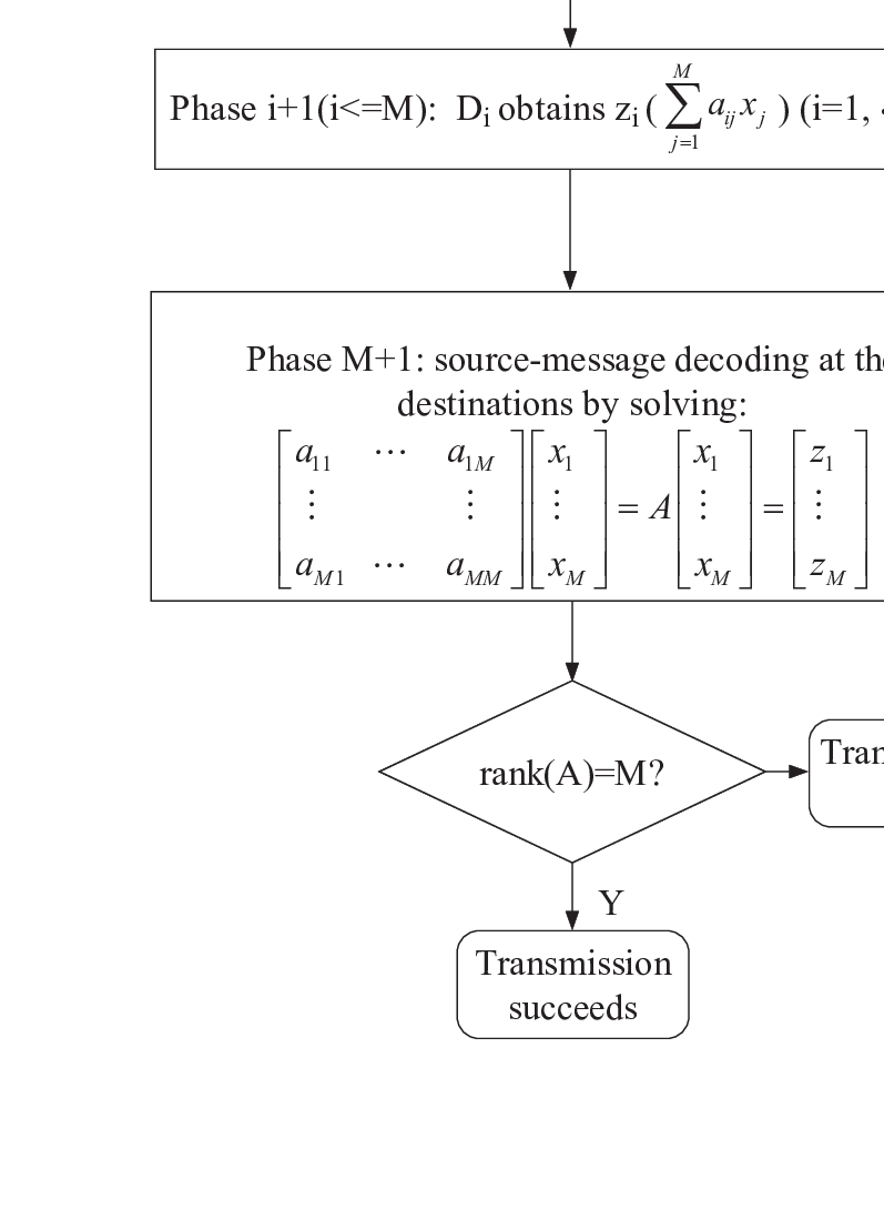
As shown in Fig. 2, a CPF based transmission protocol consists of phases. The detailed procedure for the case 11 1 It will be discussed in Section II-C for the transmission procedure for the two cases of and . is illustrated as follows.
- •
In Phase , all source nodes transmit their messages simultaneously to all the relay nodes. At the end of this phase, each relay node decodes one or more linear equations of the combination of individual transmitted messages from all sources with selected integer NC coefficient vectors.
- •
In Phase (), the th relay delivers its decoded function message to all destination nodes. At the end of Phase , all the destination nodes decode the function message received and store it for source-message decoding at the end of Phase .
- •
Source-message decoding at the end of Phase : with decoded function messages from the relay nodes, each destination nodes tries to recover all original messages. This would be possible if sufficient amount of equations are received reliably, i.e., rank (the number of source nodes) of the matrix constructed by all these integer coefficients is achieved at each destination node.

Note that for the CPF phase (Phase 1), from [15], with the specified , the CPF rate at the th relay for the real-valued AWGN networks, achieved by lattice coding, is
| (1) |
where is the transmit power. The achievable common rate of all relays, is hence given by,
| (2) |
Correspondingly, the required transmit power at all source nodes for the th relay with the common transmit rate , i.e., , is given by,
| (3) |
where , , and . The required transmit power at all source nodes for the CPF phase is given by,
At this power level, all relays can enjoy the common computing rate .
In addition, for the achievable common CPF rate, we would like to show an interesting property of the coefficients , and related to , which is summarized in Lemma 1.
Lemma 1
With positive transmit power at relay nodes, we have
| (4) |
The proof is given in Appendix A and is omitted here.
On the other hand, for the relaying phases, the relay nodes forward the function messages to all destination nodes consecutively. Since all destination nodes need to successfully receive the function messages, the broadcast rate is determined by the minimum channel gain of the R-D links for the transmitted relay node, i.e., . Hence, the broadcast rate of the th relay is determined by,
| (5) |
II-A Case Study: A Simple Example
Consider a three-source, three-relay and three-destination network. The message transmitted by each source is () in the first hop. The first relay decodes a function message of () and forwards it to all destinations in the second hop. The second and the third relay decode function messages of () and () respectively. Hence they transmit these function messages in the third hop and the fourth hop consecutively. Assume that all destination nodes successfully receive the three function messages and attain the coefficient vectors of the three relays. To obtain the three original source messages, all destination nodes are then required to solve the following equation below.
| (6) |
To ensure the uniqueness of the solution to this matrix equation, must be a full-rank matrix, i.e., for the given case and each destination can then decode all the original messages from the sources.
Unfortunately, by letting , we have and and can not be decoded at the destinations and the entire transmission fails. The importance of selection of the coefficient vectors to guarantee is in full rank is therefore verified and we discuss it in Sec. II-B for and Sec. II-C for the general topology.
II-B Integer Coefficient Vector for the case
From the discussion above, it is observed that selection of coefficient vector is crucial for the achievable CPF rates. Hence for clarity, we shall briefly review the three methods in the literature to obtain the integer coefficient vectors. Note that all these methods in the literature were only presented for the case . For a given at the th relay, we can find by
- •
method a) (naive method): obtain the integer coefficient vector individually by solving () at the th relay, where the function returns the closest integer to .
- •
method b) (local optimal method): obtain the locally-optimal integer coefficient vector individually as in [22] with the respective at the th relay.
- •
method c) (global optimal method): obtain all the integer coefficient vectors () () at all relays by employing the jointly optimization method in [23] to ensure that the full rank requirement of the matrix constructed by the integer coefficient vectors of all relays is satisfied.
For methods a) and b), only the local channel information is required. Therefore, they can not guarantee the full rank requirement at the destination nodes, i.e., the corresponding destination node may ultimately fail to decode the source messages and lead to the failure of the entire transmission.
On the other hand, method c) can guarantee the full matrix requirement at the cost of indispensable additional signaling overhead among the relay nodes, due to the joint optimal search procedure. It is therefore expected to perform better than method a) and b) at the sacrifice of higher overhead.
II-C General Scenario
From the case study in II-A, for the general M-source multicast network, we must also have to decode all source messages at the destinations, as shown in Fig. 3. It is readily concluded that at least transmissions are required by the relay nodes. However, if more than relay transmissions are allowed, it incurs inefficient spectrum resource usage and the throughput is decreased. In this sense, we only allow (the number of source nodes) relay phases over the R-D transmissions in this paper.
Therefore, if , we can always select the best relays for transmission. For instance, method b) can be extended in this case by selecting the best relays with the highest achievable CPF rates among all relays in an descending order. For an extended method c), however, we need to select the best vectors with their highest achievable CPF rates among all relays in an descending order, with the constraint that the corresponding coefficient vectors linearly independent.
For the case that , by letting some relays to decode more linear combined messages in the first phase (selecting more than one ), relay transmission phases are also attainable to make the destinations capable of decoding all source messages. For example, an implementation algorithm employing an extended method c) is given as follows.
- •
At the end of Phase 1, each relay node tries to decode a number of function messages with the corresponding achievable CPF rates.
- •
Each relay node broadcasts its achievable rates and the message index to a central controller and it lists different CPF rates in an descending order and selects the highest CPF rates with their coefficient vectors linearly independent.
- •
The central controller notifies each relay its selected rates and the associated message index, followed by the M relaying transmission phases.
Hence, for the case , some relay nodes with higher CPF rates may need to transmit in multiple slots.
In the following, we seek to find the fundamental limit on the optimal common multicast throughput over the delay-stringent and the delay-tolerant scenarios respectively. It is emphasized that the considered relaying phases still consists of phases. As discussed above, it follows from the full rank requirement of the constructed matrix if and more efficient usage of spectrum resources if . Hence, in this work, we only allow relaying phases.
III Delay-Stringent Transmission
In this section, we shall address the achievable common multicast throughput with CPF under stringent delay constraints, i.e., messages must be delivered within one slot from the source nodes to the destination nodes. In this case, the aim is to maximize the achievable common multicast throughput by optimally allocating the time resources to each phase within each slot. This can be applied to some realtime communication applications with the minimum rate requirement within each slot.
Firstly, we denote as the time fraction assigned to the first phase for S-R transmission with CPF and as the time fraction allotted to the th phase or the th relay for transmission. In addition, and are denoted as the transmit powers of each source node at the first phase (compute-and-forward phase) and the th relay, respectively. We also denote and as the transmit rate of the corresponding phase. Hence, the products and are the throughput of the CPF phase and the th relay phase, respectively. The end to end throughput per slot is hence determined by the minimum of the throughput of all phases, namely, ().
Based on the above analysis, the optimization problem within one slot for given channel coefficients of all links, termed as P1, is formulated as follows,
| (7) |
where . The associated power constraint and the physical constraint are given as follows.
| (8) | |||
| (9) | |||
| (10) |
where the objective function in (7) is to maximize the minimum throughput of each phase. (8) and (9) give the power constraint of the CPF phase and the th relaying phase. Hence, by transmitting at , each phase achieves its optimal rate.
Generally speaking, this is a max-min optimization problem and seems difficult in the first glance. We hence rewrite P1 in an equivalent form as follows,
| (11) |
subject to
| (12) |
and the physical constraint in (10). This follows from the fact that the achievable rate is an increasing function of the transmit power and hence to achieve optimality requires transmission with the highest power allowed. This is however a simple linear optimization problem and the solution to P1 is given by,
| (13) | |||
| (14) | |||
| (15) |
where the asterisk denotes optimality and is the optimal achievable common multicast throughput with given channel coefficients in delay-stringent applications.
Note that here we consider the simple case that the average power constraint at each node is imposed as the constraint for each node for the discussed slot, with the aim to optimize the throughput within each slot.
Remark 1
A typical application of it is the realtime multicast multimedia which requires the minimum data rate for the discussed slot. Another typical case would be a very slow fading scenario where channels can be regarded as quasi-static. For other applications without the minimum rate constraint or in a relatively fast fading environment, a possible extension of P1 is to optimize the throughput within multiple slots by allocating different power resources to each slot due to channel variations while still maintaining the delay-stringent constraint, such that the throughput can be improved.
IV Delay-Tolerant Transmission
In this section, we shall address the performance achievable by employing compute-and-forward with full channel state information available at the transmitters. We also assume that the derived integer coefficient vectors of all relays are available at all the destination nodes. As it is, all these messages can be obtained via a feedback channel in a time-sharing manner or frequency-sharing manner for each node.
For clarity, we denote as the average power consumed at each source node for the CPF phase and the average power consumed of the th relay, respectively. Correspondingly, as the average CPF rate achievable for the CPF phase and the average rate at the th relay, respectively. Note that all these values are averaged over the associated channel coefficient distributions. Hence and are the average throughput of the CPF phase and the th relaying phase, respectively. Hence, the throughput of the transmission protocol considered for the delay-tolerant scenario is given by
To achieve the optimal throughput, we hence need to adjust power and time resources allocated for each phase. The associated problem to maximize the average common multicast throughput, referred to as P2, is formulated as follows.
| (16) |
where . The associated constraints are given as follows.
| (17) | ||||
| (18) | ||||
| (19) |
The optimization problem above aims to optimally allocate time resources to different phases in order to mitigate the performance degradation caused by bottleneck links. In this sense, P2 can also be transformed into an equivalent optimization problem below
| (20) |
subject to the average power constraints in (17)-(18), and the physical constraint in (19), and
| (21) |
where (21) points out the fact that the product of average rate of each phase and the time resource allotted to that phase should be made equal for each phase for optimality. Note that it cannot be readily observed that P2 is a convex optimization problem due to the relationship between and in (3). Fortunately, it is verified that is indeed a convex function of and therefore P2 is a convex optimization problem. This observation is summarized in Theorem 1 and the proof is presented in Appendix B.
Theorem 1
P2 is a convex optimization problem.
The detailed proof is given in Appendix B and omitted here. According to Theorem 1, P2 can be solved by the Lagrangian multiplier method. The associated Lagrangian multiplier function is given by,
| (22) |
where , are the Lagrangian multipliers with respect to the power constraints of the CPF phase and the relaying phases. is the Lagrangian multiplier with respect to the rate constraint. is the Lagrangian multiplier for the physical constraint.
The KKT conditions are given by,
| (23) | ||||
| (24) | ||||
| (25) | ||||
| (26) | ||||
| (27) |
From (24), we then obtain the optimal rate as well as the allotted power for the relaying phases.
| (28) | ||||
| (29) |
where (29) can be directly obtained from the Shannon capacity formula and (28).
For the computation rate, by deriving the first derivative of to in (3) and insert it into (23) and employing some arithmetic operations, we arrive at the follow equality.
| (30) |
where and . Here we omit the subscripts of , and for simplicity and we assume that , i.e., the th offers the lowest CPF rate. By applying some arithmetic operations on (30), we arrive at a mono basic quadratic equation,
| (31) |
Therefore, the possible solutions to this quadratic equation are given by,
| (32) |
Furthermore, it can be shown that only one out of these two possible solutions to this quadratic equation is feasible.
Firstly, we consider a possible solution, . We then have
| (33) | ||||
| (34) |
Note that from Lemma 1, it is observed that . Hence this solution is infeasible.
Secondly, for the other possible solution, , we have
| (35) |
On the other hand, since
we have . Hence the feasibility of is demonstrated. We then arrive at the unique feasible solution to , which is,
| (36) |
Therefore, by replacing with , the optimal CPF rate can be obtained accordingly from (36). we hence arrive at Theorem 2.
Theorem 2
The solution to P2 is given by,
| (37) | ||||
| (38) |
where we set and assume that
Note again that the CPF rate of the th relay is assumed to be the common CPF rate of all relays with the specified channel gains22 2 The procedure to determine the common CPF rate and the specific index of the associated relay is given at the end of this page..
The associated allocated power with respect to the specified channel gains are given as follows,
| (39) | ||||
| (40) |
Note that in Theorem 2 we simply assume the th relay enjoys the minimum CPF rate, i.e., the common CPF rate. However, it may not be so in all cases. A procedure to determine the common CPF rate and the index of the associated relay is therefore given as follows.
- 1.
Initialization: set .
- 2.
- 3.
Set , go to 2).
- 4.
Output the common CPF rate, the common CPF power required as well as the index of the associated th relay.
According to Theorem 2 and the algorithm above, a multi-dimensional bisection search method can be implemented to obtain the optimal solution to P2, with the convergence conditions in (25) and (26). It is noted that, in each iteration with the estimated , (), one can readily obtain , and the associated average power consumption, we then compute and from (21) and (27) and hence from (26). After getting all parameters, we check the sign of the left hand side of (25) and update , accordingly. Following this procedure, the optimal solution to P2 can be obtained.
It should be noted that the bisection method adopted can guarantee global convergence at a very slow convergence rate of [28]. However, by carefully selecting the start intervals of the parameters, the adopted bisection algorithm is shown to be able to converge to the global optimal point in tens of iterations in simulation, which is acceptable in practical implementations.
V Simulation
We now present some simulation results to compare the achievable rates by employing CPF and DF. Full channel state information is assumed to be available at the associated transmitters. The average power constraint at all nodes are assumed to be the same in the simulation setting for simplicity. The channels are assumed to be real valued fading channels and their gains are modeled by zero mean and unit gain Gaussian variables. In addition, the noises at all nodes are additive white Gaussian variables with zero mean and unit variance. For ease of computation, we shall mainly focus on a multicast network with two source nodes, two relay nodes and two destination nodes (), if not specified.
For comparison, here we briefly give a DF protocol for a multi-source multi-relay multicast network with phases, which is,
- •
In the first th () phase, the th source node transmits its data to the th relay nodes at rate .
- •
In the th phase (), the th relay node broadcasts the data from the th source node to all destination nodes at rate .
For delay-stringent applications, the problem to maximize the common multicast throughput within one slot with DF, is formulated as P3 below.
| (41) | ||||
| (42) | ||||
| (43) | ||||
| (44) |
The solution to P3 is similar to that of P1 and is hence omitted. In addition, the average throughput for delay-stringent applications can be readily obtained by averaging over the channel distributions.
Similarly, the problem to optimize the averaged common multicast throughput for delay-tolerant applications is formulated as P4 below.
| (45) |
subject to the following constraints
| (46) | ||||
| (47) | ||||
| (48) | ||||
| (49) |
Note that P4 is a standard convex optimization problem and can be readily solved by KKT conditions. The solution to it is however omitted for brevity.
For clarity, a table describing the associated transmit strategies linked to different applications is presented below.
| ine Problem Index | Strategy | Detailed Description |
| ine P1 | CPF-DS | compute-and-forward strategy employed in the delay-stringent application |
| ine P2 | CPF-DT | compute-and-forward strategy employed in the delay-tolerant application |
| ine P3 | DF-DS | decode-and-forward strategy employed in the delay-stringent application |
| ine P4 | DF-DT | decode-and-forward strategy employed in the delay-tolerant application |
| ine |
Before presenting the performance of the proposed strategies, we would like to show the probability that the network integer vector constructed matrix is not in full rank by employing the proposed methods. It is worth mentioning that, if this matrix is not in full rank, each destination node can not recover all messages from the source nodes. Hence, full rank requirement of the network integer vectors plays a crucial role in applying CPF strategy.
In Fig. 4, the probability of rank failure of each method is shown. It is seen that with global optimization, method c) satisfies full rank requirement and the advantage of applying method c) is verified. Both method a) and method b) have non-zero failure probabilities, among which method a) has a constant failure probability since its determination criterion is independent of transmit power. Method b) is with a decreasing failure probability with the increase of transmit SNR. Interestingly, with more users at high SNR regime ( at the SNR level over 20dB), it is observed the rank failure probability of method b) is negligible. On the other hand, it is worth mentioning that using method c) requires additional overhead cost, which would be a critical obstacle for a large-scale multicast network in implementation, as each node needs to exchange some control information on how to construct a global-optimal full network coding system matrix by using CPF.
In Fig. 5, the optimal averaged common multicast throughput by using CPF strategy as well as DF strategy with delay-stringent constraints are compared over randomly generated channel realizations. It is shown that CPF-DS with the integer network channel coefficient vectors found by the global optimal method, i.e., method c), outperforms that with the local optimal method (method b)) and the naive method (method a)). It is also observed that CPF-DS employing method c) outperforms DF in terms of achievable throughput. However, it is seen that CPF-DS with method a) or b) performs worse than DF strategy, due to their non-negligible rank failure probabilities as shown in Fig. 4.
In Fig. 6, the advantage of optimal time allocation is shown for delay-stringent case. It is observed that the performance of CPF-DS can be greatly improved with optimal time resource allocation. For instance, in the regime of dB transmit power for CPF-DS with method c), an additional bit/s/Hz throughput improvement is achieved by using optimal time resource allocation, compared with that using equal time-resource allocation.
In Fig. 7, the optimal common multicast throughput by using different strategies for delay-tolerant applications are shown. It is shown that CPF-DT with method c) outperforms DF strategy in terms of common throughput. For instance, in the regime of 30dB transmit power, employing CPF-DT with method c), over 10% throughput improvement is achievable, compared with DF-DT. It is also interesting to note that CPF-DT with method b) is slightly better than DF, whereas CPF-DT with method a) is worse than DF, which is due to the high probability of rank failure and the far-from-optimal integer coefficient vectors sorted by adopting method a).
Similar to Fig. 6, the advantage of optimal time allocation is shown for the delay-tolerant application in Fig. 8. With transmit power at dB, throughput is increased from roughly bit/s/Hz to over bit/s/Hz for P2 with optimal time splitting.
In Fig. 9, the achievable throughput by using CPF strategy for both the delay-stringent and delay-tolerant cases are compared. It is observed that without delay constraints, higher throughput is expected to be achievable. With transmit power at dB, an additional bit/s/Hz throughput improvement is achieved for CPF-DT compared with CPF-DS, where both of them employ method c).
In Fig. 10, we are interested in the topology with arbitrary number of relay nodes (, and ). For the case , the sole relay node needs to decode two function messages for successful source-message decoding at the destination nodes. It is observed that with less relay nodes, the optimal achievable common rate with CPF is decreased, for both the delay-stringent and delay-tolerant scenarios. This is intuitively due to the reduced cooperative diversity coming from the decreased number of relays. For the case that , it is observed that the optimal throughput of CPF is further improved than that with , which comes from the increased cooperative diversity.
On the other hand, it is also observed that with the single relay node (), the CPF strategy performs slightly worse than DF strategy for delay-tolerant case and roughly as good as DF for delay-stringent case, due to the reduced relaying diversity. Taken into account that more overhead information is required for CPF strategy, it is intuitively concluded that DF is still a good choice for transmission in a small-scale network with less potential relay nodes than source nodes.
In Fig. 11, the optimal common multicast throughput for delay-tolerant application using different strategies is shown for a four-source, four-relay and four-user multicast network (). The performance gain of employing CPF over DF is hence verified for a larger network. It is observed that CPF employing method b) performs only slightly worse than that with method c) in terms of throughput, since method b) in a larger network has a lower rank failure probability. Hence, it is intuitively learned that, it may be worthwhile to employ method b) for CPF in large networks in the medium to high SNR regime. In this way, we can not only achieve close to optimal performance as given by employing method c), but as well avoid the overhead cost incurred by employing method c).


VI Conclusion
In this work, we considered a multi-source multicast network with the aid of an arbitrary number of relay nodes. We tried to find the fundamental limit on the maximal common multicast throughput of all S-D pairs. To this end, a transmission protocol employing compute-and-forward strategy was proposed for an arbitrary number of relays. Delay-stringent transmission as well as delay-tolerant transmission applications were both investigated. The associated optimization problems were formulated and solved, through the allocation of time and energy resources. Various simulation was done for validation of the performance improvement of CPF over the conventional DF in terms of throughput. It was shown that with the increasing number of relay nodes, the CPF strategy can perform better due to the increased diversity. Finally, it was intuitively shown that, using CPF with method b) was a good choice for large networks in medium to high SNR regime, as it not only provided performance quite close to CPF with method c), but also avoided the additional communication cost incurred by using method c).
Acknowledgments
This work was partially supported by NSFC grant No. 61171064 and The National 973 Project of China grant No. 2012CB316102.
References
- [1] R. Ahlswede, N. Cai, S. Li, and R. Yeung, “Network information flow,” IEEE Tran. Inf. Theory, vol. 46, no. 4, pp. 1204–1216, 2000.
- [2] S. Li, R. Yeung, and N. Cai, “Linear network coding,” IEEE Tran. Inf. Theory, vol. 49, no. 2, pp. 371–381, 2003.
- [3] C. Fragouli, D. Katabi, A. Markopoulou, M. Medard, and H. Rahul, “Wireless network coding: Opportunities & challenges,” in Proc. IEEE Military Communi. Conf. (MILCOM’07). IEEE, 2007, pp. 1–8.
- [4] W. Li, J. Li, and P. Fan, “Network coding for two-way relaying networks over rayleigh fading channels,” IEEE Tran. Veh. Tech., vol. 59, no. 9, pp. 4476–4488, 2010.
- [5] B. Niu, H. Jiang, and H. V. Zhao, “A cooperative multicast strategy in wireless networks,” IEEE Tran. Veh. Tech., vol. 59, no. 6, pp. 3136–3143, 2010.
- [6] J. Zhang, K. Ben Letaief, P. Fan, and K. Cai, “Network-coding-based signal recovery for efficient scheduling in wireless networks,” IEEE Tran. Veh. Tech., vol. 58, no. 3, pp. 1572–1582, 2009.
- [7] T. Oechtering and H. Boche, “Stability region of an optimized bidirectional regenerative half-duplex relaying protocol,” IEEE Tran. Communi., vol. 56, no. 9, pp. 1519–1529, 2008.
- [8] Z. Chen, T. J. Lim, and M. Motani, “Energy efficiency and queue stability in a two-way relay network,” in Proc. IEEE Int. Conf. Communi. Systems (ICCS’12). IEEE, 2012, pp. 36–40.
- [9] ——, “Energy optimization for stable two-way relaying with a multi-access uplink,” in Proc. Wireless Communi. and Networking Conf. (WCNC’12). IEEE, 2012, pp. 36–40.
- [10] P. Popovski and H. Yomo, “Physical network coding in two-way wireless relay channels,” in Proc. IEEE Int. Conf. Communi. (ICC’07). IEEE, pp. 707–712.
- [11] S. Zhang, S. Liew, and P. Lam, “Physical layer network coding,” in Proc. ACM Annual Int. Conf. Mobile Computing and Networking (MobiCom’06), vol. 6. Citeseer, 2006, pp. 358–365.
- [12] S. Zhang and S. Liew, “Channel coding and decoding in a relay system operated with physical-layer network coding,” IEEE Jour. Selected Areas in Communi., vol. 27, no. 5, pp. 788–796, 2009.
- [13] D. Wang, S. Fu, and K. Lu, “Channel coding design to support asynchronous physical layer network coding,” in Proc. Global Telecommuni. Conf. (GLOBECOM’09). IEEE, 2009, pp. 1–6.
- [14] L. Lu and S. Liew, “Asynchronous physical-layer network coding,” IEEE Tran. Wireless Communi., no. 99, pp. 1–13, 2011.
- [15] B. Nazer and M. Gastpar, “Compute-and-forward: Harnessing interference through structured codes,” IEEE Tran. Inf. Theory, vol. 57, no. 10, pp. 6463–6486, 2011.
- [16] S. Katti, S. Gollakota, and D. Katabi, “Embracing wireless interference: Analog network coding,” in ACM SIGCOMM Computer Communi. Review). vol. 37, no. 4, pp. 397–408, 2007.
- [17] R. Zhang, Y. Liang, C. Chai, and S. Cui, “Optimal beamforming for two-way multi-antenna relay channel with analogue network coding,” IEEE Jour. Selected Areas in Communi., vol. 27, no. 5, pp. 699–712, 2009.
- [18] K. Narayanan, M. P. Wilson, and A. Sprintson, “Joint physical layer coding and network coding for bi-directional relaying,” in 45th Annual Allerton Conf., 2007.
- [19] B. Nazer and M. Gastpar, “Reliable physical layer network coding,” Proceedings of the IEEE, vol. 99, no. 3, pp. 438–460, 2011.
- [20] M. Xiao and M. Skoglund, “Design of network codes for multiple-user multiple-relay wireless networks,” in Proc. IEEE Int. Symp. Inf. Theory (ISIT’09). IEEE, 2009, pp. 2562–2566.
- [21] ——, “Multiple-user cooperative communications based on linear network coding,” IEEE Tran. Communi., vol. 58, no. 12, pp. 3345–3351, 2010.
- [22] A. Osmane and J.-C. Belfiore, “The compute-and-forward protocol: implementation and practical aspects,” arXiv preprint arXiv:1107.0300, 2011.
- [23] L. Wei and W. Chen, “Compute-and-forward network coding design over multi-source multi-relay channels,” IEEE Tran. Wireless Communi., vol. 11, no. 9, pp. 3348–3357, 2012.
- [24] G. Wang, W. Xiang, and J. Yuan, “Outage performance for compute-and-forward in generalized multi-way relay channels,” IEEE Communi. Let., vol. 16, no. 12, pp. 2099–2102, 2012.
- [25] R. Zamir, S. Shamai, and U. Erez, “Nested linear/lattice codes for structured multiterminal binning,” IEEE Tran. Inf. Theory, vol. 48, no. 6, pp. 1250–1276, 2002.
- [26] U. Erez and R. Zamir, “Achieving 1/2 log (1+ snr) on the awgn channel with lattice encoding and decoding,” IEEE Tran. Inf. Theory, vol. 50, no. 10, pp. 2293–2314, 2004.
- [27] D. Gunduz, A. Yener, A. Goldsmith, and H. V. Poor, “The multi-way relay channel,” in IEEE Int. Symp. Inf. Theory (ISIT’09). IEEE, 2009, pp. 339–343.
- [28] E. Cheney and D. Kincaid. Numerical mathematics and computing. Cengage Learning, 2012.
Appendix A Proof of Lemma 1
From (), it is observed that and must be both positive or negative, as long as the transmit power is positive. Hence there are two possible scenarios:
- 1.
and , we then arrive at .
- 2.
and we then arrive at .
Since , we arrive at and hence only Case 2) is feasible, i.e., holds, as long as a positive transmit power is employed at the relay nodes. Since this property holds for all the relay nodes, Lemma 1 is proved.
Appendix B Proof of Convexity of P2
Here we shall prove the convexity with respect to . Suppose the th relay requires the highest source transmit power for a common CPF rate. We hence have . Therefore, we only need to show is a convex function of .
Recalling that
| (50) |
and
| (51) |
it can be observed that is a differentiable function of . Therefore, we only need to show the positivity property of its second derivative with respect to the associated CPF rate, . To proceed, the first derivative with respect to is given by,
| (52) | ||||
| (53) | ||||
| (54) |
which confirms the fact that is an increasing function of .