Dedicated to the memory of Professor Eduard Alekseevich Kuraev
Status of the lepton and effects of hadronic corrections
Abstract
The electron and muon anomalous magnetic moments (AMM) are measured in experiments and studied in the Standard Model (SM) with the highest precision accessible in particle physics. The comparison of the measured quantity with the SM prediction for the electron AMM provides the best determination of the fine structure constant. The muon AMM is more sensitive to the appearance of New Physics effects and, at present, there appears to be a three- to four-standard deviation between the SM and experiment. The lepton AMMs are pure relativistic quantum correction effects and therefore test the foundations of relativistic quantum field theory in general, and of quantum electrodynamics (QED) and SM in particular, with highest sensitivity. Special attention is paid to the studies of the hadronic contributions to the muon AMM which constitute the main source of theoretical uncertainties of the SM.
pacs
13.40.Em, 11.15.Pg, 12.20.Fv, 14.60.EfI Motivation
The anomalous magnetic moment (AMM) of charged leptons () is defined by
| (1) |
with the gyromagnetic ratio of the lepton magnetic moment to its spin, in Bohr magneton units. For a free pointlike fermion one has in accordance with the Dirac equation (Fig. 1a). However, deviations appear when taking into account the interactions leading to fermion substructure and thus to nonzero (Fig. 1b-g).
During the first years of the lepton AMM studies the fundamental task was to test the foundations of quantum field theory in general and quantum electrodynamics (QED) in particular. At present, the measurements of the lepton AMM are one of the major low-energy tests of the standard model (SM) and play an important role in the search for new interactions beyond the SM.

The nonzero lepton AMMs are induced by radiative corrections due to the coupling of the lepton spin to virtual fields, which in the SM are induced by QED, weak and strong (hadronic) interactions11 1 For comprehensive reviews see [1, 2]. (Fig. 1)
| (2) |
The electron and muon AMMs are among the most accurately measured quantities in elementary particle physics. Today, the electron AMM serves as the best quantity to determine the fine structure constant with the highest accuracy. At the same time, for , there is a deviation at the level of 3-4 of the SM prediction from the measured value. Even if this does not give a clear indication for the existence of New Physics, it allows us to provide stringent constraints on the parameters of hypothetical models.
The outline of this paper is as follows. In Section 2, we briefly report on the status of the electron AMM. In Section 3, the latest experimental and theoretical results on are presented. In Section 4, we review the most problematic theoretical input coming from the contribution due to the hadronic light-by-light (HLbL) scattering mechanism. Section 5 is devoted to some technical details of the calculations of the HLbL within the nonlocal chiral quark model (NQM). Conclusions are presented in the last Section.
II Electron AMM and fine structure constant
In 2008, the unique measurement by the Harvard group of Prof. G. Gabrielse, using a one-electron quantum cyclotron, obtained the electron AMM with unprecedented accuracy [3]
| (3) |
This result leads to the determination of the fine structure constant with the extraordinary precision [4, 5]
| (4) |
The latter became possible after the complete QED contribution to the electron AMM up to tenth order in the coupling constant were achieved numerically by the Prof. T. Kinoshita group [4] (for recent review see [5]). Note, that the uncertainty in (4) is dominated by the uncertainty in the measurement of .
The value in (4) has the highest precision of any value of currently available [6]. Thus, a new measurement [7] of the ratio between the Planck constant and the mass of atom studied by atom recoil leads to a value of the fine structure constant [6] By using this one gets for the electron AMM
| (5) |
that is in agreement with the measurement (3).
III Muon AMM: experiment vs theory
In 2006, the results on the measurements by the E821 collaboration at Brookhaven National Laboratory [8] were published. The combined result, based on nearly equal samples of positive and negative muons, is22 2 Lateron this value was corrected [6] for a small shift in the ratio of the magnetic moments of the muon and the proton as
| (6) |
This exiting result is still limited by the statistical errors and proposals to measure with a fourthfold improvement in accuracy have been proposed at Fermilab (USA) [9] and J-PARC (Japan) [10]. A future experiments plan to reduce the present experimental error to a precision of ppm.
In the SM the dominant contribution to the lepton AMM comes from QED (Fig. 1b). The complete tenth-order QED contribution to was reported in [11]
| (7) |
The accuracy of these calculations is enough for any planed experiments in new future.
In general, the weak contributions (Fig. 1c) are small due to suppressing factor , where is a typical mass of heavy and bosons. The one- and two-loop evaluations indicate that they are known with a sufficiently high accuracy [12, 13]
| (8) |
where the remaining theory error comes from the unknown three-loop contributions and dominantly from light hadronic uncertainties in the second-order electroweak diagrams with quark triangle loops. The most important feature of these new estimates, that significantly increase the theoretical precision, is to use the LHC result on the Higgs-boson mass measured by ATLAS [14, 15] and CMS [16, 17] Collaborations.
Strong (hadronic) interaction produces relatively small contributions to , however they are known with an accuracy comparable to the experimental uncertainty in (6). In leading in orders, these contributions can be separated into three terms
| (9) |
In (9), is the leading in contribution due to the hadron vacuum polarization (HVP) effect in the internal photon propagator of the one-loop diagram (Fig. 1d), is the next-to-leading order contribution related to iteration of HVP (Fig. 1e). The last term is not reduced to HVP iteration and it is due to the hadronic light-by-light (HLbL) scattering mechanism (Fig. 1g).
The hadronic contributions in (9) are determined by effects dominated by the long distance dynamics, the region where the methods of perturbation theory of Quantum Chromodynamics (QCD) do not applicable and one must use less reliable nonperturbative approaches. However, in case of HVP, using analyticity and unitarity (the optical theorem) can be expressed as the spectral representation integral [18]
| (10) |
which is a convolution of the hadronic spectral function
| (11) |
with the known from QED kinematical factor
| (12) |
where is the muon mass. The QED factor is sharply peaked at low invariant masses and decreases monotonically with increasing . Thus, the integral defining is sensitive to the details of the spectral function at low . At present there are no direct theoretical tools that allow one to calculate the spectral function at low with required accuracy. Fortunately, is related to the total hadrons cross-section at center-of-mass energy squared by
| (13) |
and this fact is used to get quite accurate estimate of . The most precise recent phenomenological evaluations of , using recent data, provide the results
| (14) |
In addition, the data on inclusive decays of the -lepton into hadrons are used to replace the data in certain energy regions. This is possible, since the vector current conservation law relates the part of the electromagnetic spectral function to the charged current vector spectral function measured in +non-strange hadrons (see, i.e. [21]). All these allow one to reach a substantial improvement in the accuracy of the contribution from the HVP during the last decade.
Similarly, the dispersion relation approach and the same phenomenological input lead to the estimate of the next-to-leading hadronic contribution (Fig. 1e) [20]
| (15) |
Thus, the HVP and next-to-leading order contribution related to HVP are known with an accuracy better than 1 per cent.
In near future, it is expected that new and precise measurements from CMD3 and SND at VEPP-2000 in Novosibirsk, BES III in Beijing and KLOE-2 at DAFNE in Frascati allow one to significantly increase the accuracy of predictions for and and resolve some inconsistency problems between different set of data.
Combining all SM contributions one obtains
| (16) |
where we take the leading order evaluations given in (14a) and the guessed value for the hadronic light-by-light contribution from [22]
| (17) |
The latter contribution will be discussed below with detail. The resulting difference between the experimental result (6) and the full SM prediction is
| (18) |
which signals an discrepancy between theory and experiment. The SM theoretical error is dominated by the hadronic contributions. In that respect, theoretical predictions of HVP and HLbL contributions to should be of the same level or better than the precision of planed experiments.
IV Status of the hadronic light-by-light scattering contribution to
The next-to-leading order corrections are suppressed by the absolute value by an extra degree of . However, one kind of these contributions, corresponding to the HLbL (Fig. 1g), is of the amount ranging from 0.5 to 1.5 ppm and known with accuracy of order 50%. It gives an error comparable in magnitude with the uncertainty induced by HVP (14). The problem is that the HLbL scattering contribution can not be calculated from first principles or (unlike to HVP) directly extracted from phenomenological considerations. Instead, it has to be evaluated using various QCD inspired hadronic models that correctly reproduce low- and high- energy properties of the strong interaction. Nevertheless, as will be discussed below, it is important for the model calculations that phenomenological information and well established theoretical principles should significantly reduce the number of model assumptions and the allowable space of model parameters.
In general, the HLbL scattering amplitude is a complicated object for calculations. It is the sum of different diagrams including the dynamical quark loop, the meson exchanges, the meson loops and the iterations of these processes. Fortunately, already in the first papers devoted to the calculation of the HLbL contributions [23, 24, 25], it has been recognized that these numerous terms show a hierarchy. This is related to the existence of two small parameters: the inverse number of colors and the ratio of the characteristic internal momentum to the chiral symmetry parameter . The former suppresses the multiloop contributions, so that the leading contribution is due to the quark loop diagram and the two-loop diagrams with mesons in the intermediate state. In latter case, the contribution of the diagram with intermediate pion is enhanced by small pion mass in the meson propagator.
Different approaches to the calculation of the contributions from the HLbL scattering process to were used. These approaches can be separated in several groups. The first one consists of various extended versions of the vector meson dominance model (VMD) supplemented by ideas of the chiral effective theory, such as the hidden local symmetry model (HLS) [24], the lowest meson dominance (LMD) [26, 27, 28], the resonance chiral theory (RT) [29, 30]. The second group is based on the consideration of effective models of QCD that use the dynamical quarks as effective degrees of freedom. The latter include different versions of the (extended) Nambu–Jona-Lasinio model (E)NJL [25, 31], the Constituent Quark Models with local interaction (CQM) [32, 33, 34, 35], the models based on nonperturbative quark-gluon dynamics, like the non-local chiral quark model (NQM) [36, 37], the Dyson-Schwinger model [39] (DS), or the holographic models (HM) [40, 41]. The lattice calculations of HLbL are still at an exploratory stage [42].
The results of the model calculations are given in Tables 1 and 2. Table 1 contains the model results where few sources of contributions can be identified33 3 The NQM results for the pion and pseudoscalar mesons exchanges are taken from [36]. The scalar mesons contribution is corrected value of (from [37] to [38]). The dynamical quark-loop contribution and the total result are taken from [38].. In Table 2 there are the model results where only contribution of the light pseudoscalar mesons is calculated.
To reduce the model dependence of various approaches, different constraints on their parameter space are employed. One kind of important constraints on the models follows from the phenomenology of the two-photon widths of the pseudoscalar mesons and their transition form factors first emphasized in [24]. Another set of constraints follows from the large momentum asymptotics for the meson transition form factors [24, 25, 26] and for the total light-by-light scattering amplitude considered in [27, 36, 37], obtained using perturbative QCD and reproduced within the NQM.
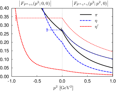
In addition, the model amplitudes have to be consistent with the 4-momentum conservation law. In practice, it means that the off-shell effects for intermediate mesons should be taken into account [1, 36, 37]. For illustration of this effect see Fig. 2 from [36].
Finally, the model calculations should be tested by reproducing the dispersion analysis result for the HVP contribution to as it was done in [23, 43, 32, 44, 35] and the known (semi)analytical results on the fermion-loop contributions to the lepton AMM as it was done in [32, 34, 37, 35]. In this respect note, that in [45] the CQM expression of [34] for the 4-loop HLbL contribution to the was used for analytical evaluation of the first term of eighth-order contribution to and and contributions to . The analytical results turned out to be in good agreement with the numerical results of calculations of these 8-th order massive corrections, re-evaluated in the process of obtaining 10-th order corrections to in [4] and complete 10-th order corrections to [11]. In [45] the statement was made, that the comparison of the results obtained in [45] with the numerical calculations of the 8-order massive dependent corrections indicate that the numerical results are also sensitive to higher order power-suppressed massive-dependent corrections. This statement was confirmed by direct analytical calculations, performed recently in [46]. These QED calculations of [45] and [46] and the comparison with the results of numerical 8-th order QED calculations of [4] demonstrate, that the CQM calculations of 8-th order light-by-light contributions to of [34] are correct.
| Model | PS | S | AV | Quark | Total | ||
|---|---|---|---|---|---|---|---|
| loop | loops | ||||||
| VMD (Hayakawa [24]) | |||||||
| ENJL (Bijnens [25]) | |||||||
| LMD+V (Knecht [26]) | |||||||
| Q-box (Pivovarov [32]) | |||||||
| LENJL (Bartos [31]) | |||||||
| (LMD+V)′(Melnikov [27]) | |||||||
| NQM (Dorokhov [36, 37, 38]) | |||||||
| oLMDV (Nyffeler [28]) | |||||||
| DS (Goecke [39]) | |||||||
| CQM (Greynat [35]) |
| Model | PS | |
|---|---|---|
| Holography (Hong [40]) | ||
| Holography (Cappiello [41]) | ||
| RT (Kampf [29]) | ||
| RT (Roig [30]) |
In the next part we discuss the HLbL contribution as it is calculated within the NQM and show that, within this framework, it might be possible to realistically determine this value to a sufficiently safe accuracy. We would like to discuss, how well this model (see, e.g., [47]) does in calculating . Below, within the NQM, we discuss in some details the theoretical status of HLbL contributions to due to the exchange by light mesons and the dynamical quark loop.
V HLbL contribution to the muon AMM within nonlocal chiral quark model
V.1 NQM dynamics
The NQM is an effective QCD inspired model that has a numerous applications for description of low energy hadronic dynamics [47]. We mention only those applications that are related to the problem of hadronic contributions to . The two-point VV correlator has been calculated in [48] and used for calculations of [44]. The three-point VAV correlator has been studied in [49] and used for calculations of the hadronic photon--boson vertex contribution to [50]. The HLbL corrections due to light meson exchanges and specific HVP corrections, where the virtual photon splits into and , was elaborated in [36, 37]. Note that the NQM approach in many ways similar to ENJL [25] and DS [39] models with, of course, subtle differences between all of them.
The Lagrangian of the chiral quark model has the form
| (19) |
where are the quark fields, is the diagonal matrix of the quark current masses, and are the four- and six-quark coupling constants. Second line in the Lagrangian represents the Kobayashi–Maskawa–t‘Hooft determinant vertex with the structural constant
where are the Gell-Mann matrices for and .
The nonlocal structure of the model is introduced via the nonlocal quark currents
| (20) |
where for the scalar and for the pseudoscalar channels, , and is a form factor with the nonlocality parameter reflecting the nonlocal properties of the QCD vacuum.
The model (19) can be bosonized using the stationary phase approximation which leads to the system of gap equations for the dynamical quark masses
| (21) |
with and and is the quark loop integral
where , is the dynamical quark propagator obtained by solving the DS equation, is the nonlocal form factor in the momentum representation.


The quark-meson vertex functions and the meson masses can be found from the Bethe-Salpeter equation Fig. 3. For the separable interaction (19) the quark-antiquark scattering matrix in each ( or ) channels becomes
| (22) |
where are the momenta of external quark lines, and are the corresponding matrices of the four-quark coupling constants and the polarization operators of mesons (). The meson masses can be found from the zeros of determinant The -matrix for the system of mesons in each neutral channel can be expressed as
| (23) |
where are the meson masses, are the vertex functions . The sum in (23) is over full set of light mesons: in the pseudoscalar channel and in the scalar one.
V.2 External photon fields
The gauge-invariant interaction with an external photon field can be introduced through the Schwinger phase factor
| (24) |
Then, apart from the kinetic term, the additional terms in the nonlocal interaction are generated via
| (25) |
which induces the quark-antiquark–-photon vertices. Additionally, there appear the meson–quark-anti-quark–-photon vertices. The following equations are used for obtaining the nonlocal vertices [51]
| (26) |
As an example, the quark-antiquark vertices with one-photon (Fig. 4a) and two-photon (Fig. 4b) insertions are
| (27) |
| (28) | |||
| (29) | |||
where the finite-difference derivatives are introduced
| (30) | |||||
| (31) |
In (27-29), is the momentum of incoming quark, are the momenta of incoming photons and . The vertex satisfies the Ward-Takahashi identity for dynamical quarks
| (32) |
with
| (33) |
and for the multi-photon nonlocal vertices one has
| (34) | |||

 (a)
(b)
(a)
(b)
V.3 Hadronic Light-by-light contribution to within NQM


The basic element for the calculations of is the fourth-rank light quark hadronic vacuum polarization tensor
| (35) | ||||
where are the light quark electromagnetic currents and is the QCD vacuum state. The muon AMM can be extracted by using the projection [52]
where
| (36) |
with is the muon mass, and it is necessary to make the limit .
In the NQM, the tensor is represented in the leading in order by the chain of diagrams schematically depicted in Fig. 5. In the higher order contributions, the suppression factor coming from the four-quark interaction (19) is compensated by the factor from the color trace of the quark loop. This infinite series of quark loop diagrams is summed up leading to the quark box and the diagrams with light meson exchanges. The double chain summation generates the meson loop contributions which are, however, suppressed by factor.
The HLbL contribution due to exchange of pseudoscalar (PS) and scalar (S) mesons (Fig. 6) was elaborated in [36]. The vertices containing the virtual (off-shell) meson with momentum and two virtual photons with momenta and the polarization vectors can be written as [31]

|

|

|
| (a) | (b) | (c) |
| (37) |
where for the pseudoscalar mesons
| (38) |
and for the scalar mesons
| (39) |
and the Lorentz structures are
| (40) | |||
and . The subject of model calculations [36] is to get the (PS/S)∗V∗V∗ vertex functions .

|
= |

|
+ |

|
+ |

|
+ |

|
+ |

|
+ |

|
| (a) | (b) | (c) | (d) | (e) | (f) | (g) |
The expression for from the light meson exchanges can be written in a three-dimensional integral representation as follows
| (41) | |||
where , . The universal kinematic factors and obtained after averaging over the directions of muon momentum can be found in [1] and [36], correspondingly. We would like to stress that the integral representation is valid for any form factors .
For numerical estimations in the NQM we use the Gaussian nonlocal form factor
| (42) |
Concerning the model parameters, the dynamical quark mass is taken in the typical interval 200–350 MeV and then other parameters (the current quark masses and the nonlocality parameter ) are fitted by the pion mass and the two-photon decay constant in correspondence with the pion lifetime given within the error range of PDG in [53]. The results are given in Table 1. Within the NQM, we found that the pseudoscalar meson contributions to are systematically lower then the results obtained in the other works. The full kinematic dependence of the vertices on the pion virtuality44 4 Later, this dependence has also been studied in [39]. diminishes the result by about 20-30% as compared to the case where this dependence is neglected. For and mesons the results are reduced by factor about 3 in comparison with the results obtained in other models where the kinematic dependence was neglected (see Fig. 2). The scalar mesons contribution is small and partially compensates model dependence of the pseudoscalar contribution (Fig. 8).

The NQM estimate for the contribution of the dynamical quark box to 55 5 The details of the calculations of the box diagram in NQM will be presented elsewhere [38]., including the contact terms (see Fig. 9), is given in Table 1. One can see that the momentum dependent dynamical mass leads to increasing of contribution of diagram with pure local quark–anti-quark–photon vertices in comparison with constant quark mass. This behavior can be expected since . The specific feature of these calculations is that there is strong compensation between the contributions from the box diagram with dynamical quarks and local vertices the box diagrams with at least one nonlocal vertex and all other types of nonlocal diagrams with contact vertices.

VI Conclusions
We briefly discussed the current status of the experimental and theoretical results on the electron and muon AMM, . These quantities, measured and calculated with very high accuracy, provide a very hard test of the SM. In particular, the electron AMM tests QED at very short distances now provides the best determination of the fine structure constant . The muon AMM is much more sensitive to the effects of the Physics beyond the SM. Presently, there is a mismatch between the latest experimental BNL measurements and SM calculations at the level of 3-4 . It is the largest deviation in elementary particle physics from the SM predictions. This may be an evidence for the existence of new interactions and stringently constrains the parametric space of hypothetical interactions extending the SM. Nowdays, the interest in this problem became lively again in view of the preparation of new Fermilab and J-PARC experiments planning to achieve a measurement precision at the 0.14 ppm level. On the other hand, the biggest theoretical uncertainty is due to the hadronic part of , especially from HVP and HLbL. In this work we considered the latest achievements in phenomenological and model approaches to estimate the leading and next-to-leading order hadronic corrections to . Further studies are needed in order to get a better control over the hadronic corrections and reach a precision of calculations comparable to or better than the experimental one.
We thank Yu.M. Bystritskiy, A.L. Kataev, N.I. Kochelev, E.A. Kuraev, V.P. Lomov, A. Nyffeler, H.-P. Pavel, A.A. Pivovarov for critical remarks and illuminating discussions. This work is supported in part by the Russian Foundation for Basic Research (projects No. 11-02-00112 and 12-02-31874).
References
- [1] F. Jegerlehner, A. Nyffeler,Phys. Rept. 477, 1 (2009).
- [2] J.P. Miller, E. de Rafael, B. L. Roberts and D. Stuckinger, Ann. Rev. Nucl. Part. Sci. 62, 237 (2012).
- [3] D. Hanneke, S. Fogwell and G. Gabrielse, Phys. Rev. Lett. 100 , 120801 (2008).
- [4] T. Aoyama, M. Hayakawa, T. Kinoshita and M. Nio, Phys. Rev. Lett. 109 , 111807 (2012).
- [5] T. Kinoshita, Int. J. Mod. Phys. A 29, 1430003 (2014).
- [6] P.J. Mohr, B.N. Taylor and D.B. Newell (CODATA Recommended Values of the Fundamental Physical Constants: 2010) Rev. Mod. Phys. 84, 1527 (2012).
- [7] R. Bouchendira, P. Clade, S. Guellati-Khelifa, F. Nez and F. Biraben, Phys. Rev. Lett. 106, 080801 (2011).
- [8] G.W. Bennett, et al. [Muon (g-2) Collaboration], Phys.Rev. D73, 072003 (2006).
- [9] G. Venanzoni [Fermilab E989 Collaboration], J. Phys. Conf. Ser. 349 (2012) 012008. E989 experiment at Fermilab: http://gm2.fnal.gov/
- [10] N. Saito [J-PARC g-2/EDM Collaboration], AIP Conf. Proc. 1467, 45 (2012).
- [11] T. Aoyama, M. Hayakawa, T. Kinoshita and M. Nio, Phys. Rev. Lett. 109 , 111808 (2012).
- [12] A. Czarnecki, W. J. Marciano and A. Vainshtein, Phys. Rev. D67 , 073006 (2003) [Erratum-ibid. D73 , 119901 (2006)].
- [13] C. Gnendiger, D. Stockinger and H. Stockinger-Kim, Phys. Rev. D88 , 053005 (2013)
- [14] G. Aad et. al. [ATLAS Collaboration], Phys. Lett. B716, 1 (2012).
- [15] G. Aad et. al. [ATLAS Collaboration], Phys. Lett. B726, 88 (2013).
- [16] S. Chatrchyan et. al. [CMS Collaboration], Phys. Lett. B716, 30 (2012).
- [17] S. Chatrchyan et. al. [CMS Collaboration], Phys. Rev. Lett. 110 , 081803 (2013).
- [18] C. Bouchiat and L. Michel, J. Phys. Radium, 22 (1961) 121; L. Durand, Phys. Rev., 128 441 (1962); M. Gourdin and E. De Rafael, Nucl. Phys. B10 , 667 (1969).
- [19] M. Davier, A. Hoecker, B. Malaescu, Z. Zhang, Eur.Phys.J. C71, 1515 (2011) [Erratum-ibid. C72 , 1874 (2012)].
- [20] K. Hagiwara, R. Liao, A. D. Martin, D. Nomura and T. Teubner, J. Phys. G38, 085003 (2011)
- [21] F. Jegerlehner, R. Szafron, Eur.Phys.J. C71, 1632 (2011).
- [22] J. Prades, E. de Rafael and A. Vainshtein, in Advanced series on directions in high energy physics, Vol. 20 [arXiv:0901.0306 [hep-ph]].
- [23] E. de Rafael, Phys. Lett. B322 (1994) 239.
- [24] M. Hayakawa, T. Kinoshita and A.I. Sanda, Phys. Rev. Lett. 75 (1995) 790; M. Hayakawa and T. Kinoshita, Phys. Rev. D57 (1998) 465 [Erratum-ibid. D66, 019902 (2002)].
- [25] J. Bijnens, E. Pallante and J. Prades, Phys. Rev. Lett. 75 (1995) 1447; J. Bijnens, E. Pallante, J. Prades, Nucl.Phys. B474, 379 (1996); B626, 410 (2002).
- [26] M. Knecht, A. Nyffeler, Phys.Rev. D65, 073034 (2002).
- [27] K. Melnikov, A. Vainshtein, Phys.Rev. D70, 113006 (2004).
- [28] A. Nyffeler, Phys.Rev. D79, 073012 (2009).
- [29] K. Kampf and J. Novotny, Phys. Rev. D84 , 014036 (2011).
- [30] P. Roig, A. Guevara and G.L. Castro, Phys. Rev. D89, 073016 (2014).
- [31] E. Bartos, A.Z. Dubnickova, S. Dubnicka, E.A. Kuraev, E. Zemlyanaya, Nucl. Phys. B632, 330 (2002).
- [32] A. A. Pivovarov, Phys. Atom. Nucl. 66 (2003) 902 [Yad. Fiz. 66 (2003) 934] [hep-ph/0110248].
- [33] J. Erler and G. Toledo Sanchez, Phys. Rev. Lett. 97, 161801 (2006).
- [34] R. Boughezal and K. Melnikov, Phys. Lett. B704, 193 (2011)
- [35] D. Greynat and E. de Rafael, JHEP 1207, 020 (2012).
- [36] A. E. Dorokhov and W. Broniowski, Phys. Rev. D 78 (2008) 073011; A.E. Dorokhov, A.E. Radzhabov, A.S. Zhevlakov,Eur. Phys. J. C71, 1702 (2011).
- [37] A.E. Dorokhov, A.E. Radzhabov, A.S. Zhevlakov, Eur. Phys. J. C72, 2227 (2012).
- [38] A.E. Dorokhov, A.E. Radzhabov, A.S. Zhevlakov, in preparation.
- [39] T. Goecke, C.S. Fischer, R. Williams, Phys.Rev. D83, 094006 (2011) [Erratum-ibid. D86 , 099901 (2012)]; Phys.Rev. D87, 034013 (2013)
- [40] D.K. Hong, D. Kim, Phys.Lett. B680, 480 (2009).
- [41] L. Cappiello, O. Cata, G. D’Ambrosio, Phys.Rev. D83, 093006 (2011).
- [42] T. Blum, A. Denig, I. Logashenko, E. de Rafael, B. Lee Roberts, T. Teubner, G. Venanzoni, [hep-ph/1311.2198].
- [43] E. Pallante, Phys. Lett. B 341 (1994) 221; B. Holdom, R. Lewis and R.R. Mendel, Z. Phys. C 63 (1994) 71; T. Goecke, C.S. Fischer and R. Williams, Phys. Lett. B 704 (2011) 211.
- [44] A.E. Dorokhov, Phys. Rev. D70, 094011 (2004).
- [45] A.L. Kataev, Phys. Rev. D86, 013010 (2012).
- [46] A. Kurz, T. Liu, P. Marquard and M. Steinhauser, Nucl. Phys. B 879 (2014) 1.
- [47] I. V. Anikin, A. E. Dorokhov and L. Tomio, Phys. Part. Nucl. 31, 509 (2000) [Fiz. Elem. Chast. Atom. Yadra 31, 1023 (2000)];
- [48] A. E. Dorokhov and W. Broniowski, Eur. Phys. J. C 32, 79 (2003).
- [49] A. E. Dorokhov, Eur. Phys. J. C 42 (2005) 309; A. E. Dorokhov, JETP Lett. 82 (2005) 1 [Pisma Zh. Eksp. Teor. Fiz. 82 (2005) 3].
- [50] A.E. Dorokhov, Acta Phys. Polon. B 36, 3751 (2005)
- [51] S. Mandelstam, Annals Phys. 19, 1 (1962); J. Terning, Phys. Rev. D44, 887 (1991).
- [52] S.J. Brodsky and E. De Rafael, Phys. Rev. 168, 1620 (1968).
- [53] J. Beringer et al. [Particle Data Group Collaboration], Phys. Rev. D 86, 010001 (2012).