Mixed Generalized Multiscale Finite Element Methods and Applications

Eric T. Chung ^†^†thanks: Department of Mathematics, The Chinese University of Hong Kong (CUHK), Hong Kong SAR. Email: tschung@math.cuhk.edu.hk. The research of Eric Chung is supported by Hong Kong RGC General Research Fund (Project 400411). Yalchin Efendiev ^†^†thanks: Department of Mathematics & Institute for Scientific Computation (ISC), Texas A&M University, College Station, Texas, USA and Center for Numerical Porous Media (NumPor), King Abdullah University of Science and Technology (KAUST), Thuwal 23955-6900, Kingdom of Saudi Arabia. Email: efendiev@math.tamu.edu. Chak Shing Lee ^†^†thanks: Department of Mathematics & Institute for Scientific Computation (ISC), Texas A&M University, College Station, Texas, USA. Email: cslee@math.tamu.edu.

Abstract

In this paper, we present a mixed Generalized Multiscale Finite Element Method (GMsFEM) for solving flow in heterogeneous media. Our approach constructs multiscale basis functions following a GMsFEM framework and couples these basis functions using a mixed finite element method, which allows us to obtain a mass conservative velocity field. To construct multiscale basis functions for each coarse edge, we design a snapshot space that consists of fine-scale velocity fields supported in a union of two coarse regions that share the common interface. The snapshot vectors have zero Neumann boundary conditions on the outer boundaries and we prescribe their values on the common interface. We describe several spectral decompositions in the snapshot space motivated by the analysis. In the paper, we also study oversampling approaches that enhance the accuracy of mixed GMsFEM. A main idea of oversampling techniques is to introduce a small dimensional snapshot space. We present numerical results for two-phase flow and transport, without updating basis functions in time. Our numerical results show that one can achieve good accuracy with a few basis functions per coarse edge if one selects appropriate offline spaces.

keywords

multiscale, mixed finite element, porous media, two-phase flow

1 Introduction

In many applications, one encounters multiple scales and high contrast. For example in subsurface applications, the media properties, such as permeability, have multiple scales and features, such as fractures and shale layers, which have thickness that are much smaller than the domain size. The solution techniques for such problems require some type of model reduction that allows reducing the degrees of freedom. Investigators developed many approaches, such as upscaling and multiscale methods, for this purpose. In these approaches, a coarse grid with a reduced number of degrees of freedom represents the solution. For example, in upscaling methods [12, 21], one typically upscales the media properties and solves the global problem on a coarse grid. In multiscale methods [1, 4, 16, 19, 20, 11, 10, 9, 18], one constructs multiscale basis functions and solves the problem on a coarse grid.

In this paper, our interest is in developing multiscale mixed methods for flows in heterogeneous media. Some earlier pioneering works in multiscale mixed finite element methods are reported in [7, 2, 3] (see also [4] for mortar multiscale construction). The motivation for using a mixed finite element framework is to preserve mass conservation, a property that is very important for flow problems. In multiscale methods, mixed methods also provide rapid evaluation of the fine-scale conservative velocity without doing a post-processing step. The main idea of mixed multiscale finite element methods is to compute multiscale basis function for each edge supported in two coarse blocks that share this common edge (see Fig. 1 for illustration). Computing one basis function per coarse edge using local or global information limited most previous approaches. As discussed in our recent paper [14, 13, 8] (in the framework of continuous Galerkin approach), one basis function per edge is not sufficient to capture many disconnected multiscale features; and therefore, one needs a systematic procedure for enriching the coarse space. Here, we follow the framework of the Generalized Multiscale Finite Element Method introduced in [14].

The main idea of the GMsFEM is to divide the computation into offline and online stages. In the offline stage, we construct (1) a snapshot space and (2) the offline space via spectral decomposition of the snapshot space. The main concept of constructing the snapshot space is that the snapshot vectors preserve some essential properties of the solution and provide a good approximation space. The main idea of the offline space is that it gives a good solution approximation with fewer basis functions. The main difficulty in the GMsFEM is in finding an appropriate snapshot space and the local spectral decomposition of the snapshot space that can give a good approximation of the solution with a fewer basis functions. We address these issues in this paper.

We construct the velocity field for the snapshot and offline spaces for the mixed GMsFEM. For approximating the pressure field, we use piecewise constant basis functions (cf. [7, 1, 3]). The snapshot solutions consist of local solutions with a unit-variable flux, chosen at all possible locations, on the internal boundary. To construct the offline space, we consider several spectral problems based on the analysis and provide a justification. We also provide an alternative derivation of the local eigenvalues problem, where each next vector in the offline space is furthest from the space of previously selected offline vectors. Some of the advantages of the mixed GMsFEM (over the continuous Galerkin GMsFEM) are the following: (1) no need for partition of unity; (2) mass conservative and useful for flow and transport. We also study oversampling techniques (cf. [17]) by constructing snapshot vectors as the local solutions in larger regions that contain the interfaces of two adjacent coarse blocks. This allows obtaining a much smaller dimensional snapshot space and can help to improve the accuracy of the mixed GMsFEM. Oversampling technique can be particularly helpful for problems with scale separation. This is because by taking the restriction of the local solutions in larger domains in the interior, we avoid the pollution effects near the boundaries.

We present numerical results for various heterogeneous permeability fields and show that we can approximate the solution using only a few basis functions. We use our approach for solving two-phase flow and transport equations. In two-phase flow and transport, we solve the flow equation for each time step and employ the fine-scale velocity to advance the saturation front. In our numerical results, we solve the flow equation without modifying multiscale basis functions, i.e., we solve the flow equation on a coarse grid. We show how adding a few extra basis functions can improve the prediction accuracy.

We organize the paper as follows. In Section 2, we present a basic model problem, fine-scale discretization, and the definitions of coarse and fine grids. In Section 3, we describe the construction of the snapshot and offline spaces. We devote Section 4 to analyzing the mixed GMsFEM. The use of oversampling techniques for the snapshot space is presented in Section 5. We present numerical results in Section 6. The paper ends with a conclusion.

2 Preliminaries

We consider the following high-contrast flow problem in mixed formulation

\displaystyle\begin{split}\kappa^{-1}v+\nabla p&=0\quad\text{in}\quad D,\\ \text{div}(v)&=f\quad\text{in}\quad D,\end{split}

(1)

with non-homogeneous Neumann boundary condition $v\cdot n=g$ on $\partial D$ , where $\kappa$ is a given high-contrast heterogeneous permeability field, $D$ is the computational domain, and $n$ is the outward unit-normal vector on $\partial D$ .

In the mixed GMsFEM considered in this paper, we construct the basis functions for the velocity field, $v=-\kappa\nabla p$ . For the pressure $p$ , we will use piecewise constant approximations. To describe the general solution framework for the model problem (1), we first introduce the notion of fine and coarse grids. We let $\mathcal{T}^{H}$ be a usual conforming partition of the computational domain $D$ into finite elements (triangles, quadrilaterals, tetrahedrals, etc.), called coarse-grid blocks, where $H>0$ is the coarse mesh size. We refer to this partition as the coarse grid and assume that each coarse-grid block is partitioned into a connected union of fine-grid blocks, which are conforming across coarse-grid edges. The fine grid partition will be denoted by $\mathcal{T}^{h}$ , which by definition is a refinement of $\mathcal{T}^{H}$ . We use $\mathcal{E}^{H}:=\bigcup_{i=1}^{N_{e}}\{E_{i}\}$ (where $N_{e}$ is the number of coarse edges) to denote the set of all edges of the coarse mesh $\mathcal{T}^{H}$ , and $\mathcal{E}^{H}_{0}$ to denote the set of all interior coarse edges. We also define the coarse neighborhood $\omega_{i}$ corresponding to the coarse edge $E_{i}$ as the union of all coarse-grid blocks having the edge $E_{i}$ , namely,

\omega_{i}=\bigcup\{K_{j}\in\mathcal{T}^{H};~~~E_{i}\in\partial K_{j}\}.

(2)

See Fig. 1 for an example of a coarse neighborhood, where the coarse-grid edges are denoted by solid lines and the fine-grid edges are denoted by dash lines.

Fig. 1: An example of a neighborhood

\omega_{i}=K_{j}\cup K_{l}

and

\omega_{i}^{+}

associated with the coarse edge

E_{i}

Let $Q_{H}$ be the space of piecewise constant functions with respect to the coarse grid $\mathcal{T}^{H}$ . The approximation of the pressure $p$ will be obtained in this space. On the other hand, a set of multiscale basis functions for the velocity field $v$ are defined for each coarse edge $E_{i}\in\mathcal{E}^{H}$ and these basis functions are supported in the coarse neighborhood $\omega_{i}$ corresponding to the coarse edge $E_{i}$ . Specifically, to obtain a basis function for a coarse edge $E_{i}$ , we will solve a local problem in the coarse neighborhood $\omega_{i}$ with a given normal velocity on $E_{i}$ and zero normal velocity on the boundary $\partial\omega_{i}$ . Notice that we can use multiple basis functions for each coarse edge $E_{i}$ by using various choices of normal velocity on $E_{i}$ . Let $\{\Psi_{j}\}$ be the set of multiscale basis functions for the edge $E_{i}$ . We define the multiscale space for the velocity field $v$ as the linear span of all local basis functions which is denoted as

{V}_{H}=\bigoplus_{\mathcal{E}^{H}}\{\Psi_{i}\}.

We also define $V_{H}^{0}=V_{H}\cap\{v\in V_{H}\,:\,v\cdot n=0\text{ on }\partial D\}$ as a subspace of $V_{H}$ consisting of vector fields with zero normal component on $\partial D$ ; that is,

{V}^{0}_{H}=\bigoplus_{\mathcal{E}_{0}^{H}}\{\Psi_{i}\}.

Given the above spaces, the mixed GMsFEM is to find $(v_{H},p_{H})\in{V}_{H}\times Q_{H}$ such that

\displaystyle\begin{split}\int_{D}\kappa^{-1}v_{H}\cdot w_{H}-\int_{D}\text{div}(w_{H})p_{H}&=0,\quad\forall w_{H}\in{V}_{H}^{0},\\ \int_{D}\text{div}(v_{H})q_{H}&=\int_{D}fq_{H},\quad\forall q_{H}\in Q_{H},\end{split}

(3)

where $v_{H}\cdot n=g_{H}$ on $\partial D$ , and for each coarse edge $E_{i}\in\partial D$ , we have

\int_{E_{i}}(g_{H}-g)\Psi_{j}\cdot n=0

for all basis functions $\Psi_{j}$ corresponding to the edge $E_{i}$ .

In addition, we let $V_{h}\times Q_{h}$ be the standard lowest-order Raviart-Thomas space for the approximation of (1) on the fine grid $\mathcal{T}^{h}$ . Then, the fine-grid solution $(v_{h},p_{h})$ satisfies

\displaystyle\begin{split}\int_{D}\kappa^{-1}v_{h}\cdot w_{h}-\int_{D}\text{div}(w_{h})p_{h}&=0,\quad\forall w_{h}\in{V}_{h}^{0},\\ \int_{D}\text{div}(v_{h})q_{h}&=\int_{D}fq_{h},\quad\forall q_{h}\in Q_{h},\end{split}

(4)

where $v_{h}\cdot n=g_{h}$ on $\partial D$ and $V_{h}^{0}=V_{h}\cap\{v\in V_{h}\,:\,v\cdot n=0\text{ on }\partial D\}$ . In terms of matrix representations, the above problem can be written as

\begin{split}M_{\text{fine}}\vec{V}_{h}+B_{\text{fine}}^{T}\vec{P}_{h}&=0\\ B_{\text{fine}}\vec{V}_{h}&=\vec{F}_{h},\end{split}

(5)

where $\vec{V}_{h}$ and $\vec{P}_{h}$ are vectors of coefficients in the expansions of the solutions $v_{h}$ and $p_{h}$ in the spaces $V_{h}$ and $Q_{h}$ , respectively. We remark that the fine-grid solution $(v_{h},p_{h})$ is considered as a reference solution, and we will compare the accuracy of the multiscale solution $(v_{H},p_{H})$ against the fine grid solution. Furthermore, it is easy to see that $Q_{H}\subset Q_{h}$ . We will construct the multiscale space $V_{H}$ so that $V_{H}\subset V_{h}$ . Therefore, the mixed GMsFEM can be considered as a conforming method to approximate the fine-grid solution. In the next section, we will give the construction of the multiscale basis functions and the space $V_{H}$ .

3 The construction of multiscale basis functions

In this section, we will discuss the construction of the multiscale space $V_{H}$ for the approximation of the velocity field. We will first introduce the snapshot space, which contains an extensive set of basis functions formed by solutions of local problems with all possible boundary conditions up to the fine-grid resolution. Then, we will present a space reduction technique which provides a systematic way to select the dominant modes in the snapshot space. This technique is based on a carefully designed local spectral problem giving a rapidly decaying residual. The resulting reduced space is obtained by the linear span of these dominant modes and is called the offline space. Notice that we use the terminology introduced in [14], where the notion of online space is also introduced. We emphasize that, since we consider problems without parameter dependence, the offline space is the same as the online space.

3.1 Snapshot space

In this section, we will define the snapshot space. Essentially, it is a space containing an extensive set of basis functions which are solutions of local problems with all possible boundary conditions up to the fine-grid resolution. Specifically, the functions in the snapshot space are $\kappa$ -harmonic functions of unit-flux functions. In the following, we explain the detailed constructions. Let $E_{i}\in\mathcal{E}^{H}$ be a coarse edge. We will find $(v_{j}^{(i)},p_{j}^{(i)})$ by solving the following problem on the coarse neighborhood $\omega_{i}$ corresponding to the edge $E_{i}$

\displaystyle\begin{split}\kappa^{-1}v_{j}^{(i)}+\nabla p_{j}^{(i)}&=0\quad\quad\text{in}\quad\omega_{i},\\ \text{div}(v_{j}^{(i)})&=\alpha_{j}^{(i)}\quad\text{in}\quad\omega_{i},\end{split}

(6)

subject to the boundary condition $v_{j}^{(i)}\cdot n_{i}=0$ on $\partial\omega_{i}$ , where $n_{i}$ denotes the outward unit-normal vector on $\partial\omega_{i}$ . One key feature of our proposed approach is that the above problem (6) will be solved separately in the coarse-grid blocks forming $\omega_{i}$ (see Figure 1 for illustration). Therefore, we will need an extra boundary condition on $E_{i}$ , which is discussed below. Notice that the coarse edge $E_{i}$ can be written as a union of fine-grid edges, namely, $E_{i}=\bigcup_{j=1}^{J_{i}}e_{j}$ , where $J_{i}$ is the total number of fine-grid edges on $E_{i}$ and $e_{j}$ denotes a fine-grid edge. Let $\delta_{j}^{(i)}$ be a piecewise constant function defined on $E_{i}$ with respect to the fine-grid such that it has value $1$ on $e_{j}$ and value $0$ on the other fine-grid edges; that is,

\delta_{j}^{(i)}=\left\{\begin{array}[]{ll}1,&\mbox{on $e_{j}$,}\\ 0,&\mbox{on other fine grid edges on $E_{i}$,}\end{array}\right.\quad\quad j=1,2,\cdots,J_{i}.

The remaining boundary condition on the coarse edge $E_{i}$ for the local problem (6) is then taken as

v_{j}^{(i)}\cdot m_{i}=\delta_{j}^{(i)}\quad\mbox{on $E_{j}$,}

(7)

where $m_{i}$ is a fixed unit-normal vector on $E_{i}$ . We remark that the constant $\alpha_{j}^{(i)}$ in (6) is chosen so that the compatibility condition $\int_{K_{l}}\alpha_{j}^{(i)}=\int_{E_{i}}\delta_{j}^{(i)}$ is satisfied, for all $K_{l}\subset\omega_{i}$ . We also remark that, since $v_{j}^{(i)}\cdot n_{i}=0$ on the boundary of $\omega_{i}$ , the vector field $v_{j}^{(i)}$ can be extended to the rest of the domain $D$ by defining $v_{j}^{(i)}=0$ outside $\omega_{i}$ . Furthermore, the above local problem (6) can be solved numerically on the underlying fine grid of $\omega_{i}$ by the lowest-order Raviart-Thomas element, so that the resulting velocity $v_{j}^{(i)}\in V_{h}$ (for simplicity, we keep the same notation for the discrete solution $v_{j}^{(i)}$ ).

The collection of the solutions of the above local problems generates the snapshot space. We let $\Psi^{i,\text{snap}}_{j}:=v_{j}^{(i)}$ be the snapshot fields and define the snapshot space $V_{\text{snap}}$ by

V_{\text{snap}}=\text{span}\{\Psi_{j}^{i,\text{snap}}:~~~1\leq j\leq J_{i},\quad 1\leq i\leq N_{e}\}.

To simplify notation, we will use the following single-index notation

V_{\text{snap}}=\text{span}\{\Psi_{i}^{\text{snap}}:~~~1\leq i\leq M_{\text{snap}}\},

where $M_{\text{snap}}=\sum_{i=1}^{N_{e}}J_{i}$ is the total number of snapshot fields.

Notice that each $\Psi^{\text{snap}}_{i}$ is represented on the fine grid by the basis functions in $V_{h}$ . Therefore, each $\Psi^{\text{snap}}_{i}$ can be represented by a vector $\psi_{i}^{\text{snap}}$ containing the coefficients in the expansion of $\Psi^{\text{snap}}_{i}$ in the fine-grid basis functions. Then, we define

R_{\text{snap}}=\left[\psi_{1}^{\text{snap}},\ldots,\psi_{M_{\text{snap}}}^{\text{snap}}\right],

which maps from the coarse space to the fine space.

3.2 Offline space

Following the general framework of [14], we will perform a space reduction on the snapshot space through the use of some local spectral problems. The reduced space is called the offline space. The purpose of this is to determine the important modes in the snapshot space and to obtain a smaller space for approximating the solution. In the general setting, we consider the spectral problem of finding a real number $\lambda$ and a vector field $v\in V_{\text{snap}}$ such that

a(v,w)=\lambda s(v,w),\quad\quad\forall w\in V_{\text{snap}},

(8)

where $a(v,w)$ and $s(v,w)$ are symmetric positive definite bilinear forms defined on $V_{\text{snap}}\times V_{\text{snap}}$ . We consider $s(v,w)$ as an inner product on $V_{\text{snap}}$ and define a linear operator $\mathcal{A}:V_{\text{snap}}\rightarrow V_{\text{snap}}$ by

s(\mathcal{A}v,w)=a(v,w).

We assume that the operator $\mathcal{A}$ has rapidly decaying eigenvalues. Note that one can take $\mathcal{A}$ to be a compact operator.

In practice, solving the above global spectral problem (8) is inefficient. Therefore, the dimension reduction and the construction of the offline space are performed locally. In particular, the above spectral problem is solved for each coarse neighborhood $\omega_{i}$ corresponding to the coarse edge $E_{i}$ . We let $V_{\text{snap}}^{(i)}$ be the snapshot space corresponding to the coarse edge $E_{i}$ , which is defined by

V^{(i)}_{\text{snap}}=\text{span}\{\Psi_{j}^{i,\text{snap}}:~~~1\leq j\leq J_{i}\}.

The local spectral problem is: find a real number $\lambda\geq 0$ and a function $v\in V_{\text{snap}}^{(i)}$ such that

a_{i}(v,w)=\lambda s_{i}(v,w),\quad\quad\forall w\in V_{\text{snap}}^{(i)}.

(9)

We will consider two different choices of local spectral problems. One can possibly use oversampling ideas [19, 17, 5, 15] to achieve a better convergence rate (see Section 5).

Spectral problem 1: We take

a_{i}(v,w)=\int_{E_{i}}\kappa^{-1}(v\cdot m_{i})(w\cdot m_{i}),\quad s_{i}(v,w)=\int_{\omega_{i}}\kappa^{-1}v\cdot w+\int_{\omega_{i}}\text{div}(v)\,\text{div}(w),

(10)

where we recall that $m_{i}$ is a fixed unit-normal on the coarse edge $E_{i}$ .

Spectral problem 2: We take

a_{i}(v,w)=\int_{\omega_{i}}\kappa^{-1}v\cdot w,\quad s_{i}(v,w)=\int_{E_{i}}[p_{v}][p_{w}],

(11)

where $(v,p_{v})$ and $(w,p_{w})$ are solutions of the local problem (6), and $[p]$ denotes the jump of the function $p$ .

In the following, we will focus our discussions on spectral problem 1. For spectral problem 2, we will only report its performance in Section 6 to show that it is also a promising way to obtain a reduced space.

Assume that the eigenvalues of (9) are arranged in increasing order

\lambda_{1}^{(i)}<\lambda_{2}^{(i)}<\cdots<\lambda_{J_{i}}^{(i)},

(12)

where $\lambda_{k}^{(i)}$ denotes the $k$ -th eigenvalue for the coarse neighborhood $\omega_{i}$ . The corresponding eigenvectors are denoted by $Z_{k}^{(i)}=(Z_{kj}^{(i)})_{j=1}^{J_{i}}$ , where $Z_{kj}^{(i)}$ is the $j$ -th component of the vector $Z_{k}^{(i)}$ . We will use the first $l_{i}$ eigenfunctions to form the offline space. We remark that we assume the eigenvalues are strictly increasing (here, we refer to the inverse of $\mathcal{A}$ , cf. (8)) only to simplify the discussion. In practice, if there are multiple eigenvectors corresponding to a specific eigenvalue, then we will take all these eigenvectors to be part of the basis functions when the corresponding eigenvalue is selected. Using the eigenfunctions, offline basis functions can be constructed as

\Psi_{k}^{i,\text{off}}=\sum_{j=1}^{J_{i}}Z_{kj}^{(i)}\Psi_{j}^{i,\text{snap}},\quad\quad k=1,2,\cdots,l_{i}.

The global offline space is then

V_{\text{off}}=\text{span}\{\Psi_{k}^{i,\text{off}}:~~~1\leq k\leq l_{i},\quad 1\leq i\leq N_{e}\}.

To simplify notation, we will use the following single-index notation

V_{\text{off}}=\text{span}\{\Psi_{k}^{\text{off}}:~~~1\leq k\leq M_{\text{off}}\},

where $M_{\text{off}}=\sum_{i=1}^{N_{e}}l_{i}$ is the total number of offline basis functions. This space will be used as the approximation space for the velocity; that is, $V_{H}=V_{\text{off}}$ in the GMsFEM system (3). Furthermore, we define $V_{\text{off}}^{0}$ as the restriction of $V_{\text{off}}$ formed by the linear span of all basis functions $\Psi_{k}^{\text{off}}$ corresponding to interior coarse edges only. Thus, all vectors in $V_{\text{off}}^{0}$ have zero normal component on the global domain boundary $\partial D$ .

In term of matrix representations, the above eigenvalue problem (9) can be expressed as

A_{\text{snap}}^{(i)}Z_{k}^{(i)}=\lambda_{k}^{(i)}S_{\text{snap}}^{(i)}Z_{k}^{(i)},

(13)

where

\displaystyle A_{\text{snap}}^{(i)}=[(A_{\text{snap}}^{(i)})_{mn}]=a_{i}(\Psi_{m}^{i,\text{snap}},\Psi_{n}^{i,\text{snap}})=R_{\text{snap}}^{T}A_{\text{fine}}^{(i)}R_{\text{snap}}

and

\displaystyle S_{\text{snap}}^{(i)}=[(S_{\text{snap}}^{(i)})_{mn}]=s_{i}(\Psi_{m}^{i,\text{snap}},\Psi_{n}^{i,\text{snap}})=R_{\text{snap}}^{T}S_{\text{fine}}^{(i)}R_{\text{snap}}.

We note that $A_{\text{fine}}^{(i)}$ and $S_{\text{fine}}^{(i)}$ denote analogous fine-scale matrices that use fine-grid basis functions. Notice that each $\Psi^{\text{off}}_{k}$ is represented on the fine grid. Therefore, each $\Psi^{\text{off}}_{k}$ can be represented by a vector $\psi_{k}^{\text{off}}$ containing the coefficients in the expansion of $\Psi^{\text{off}}_{k}$ in the fine-grid basis functions. Then, we define

R_{\text{off}}=\left[\psi_{1}^{\text{off}},\ldots,\psi_{M_{\text{off}}}^{\text{off}}\right],

which maps from the offline space to the fine space. Similar to (5), the GMsFEM system (3) can be represented in matrix form as follows.

\begin{split}R_{\text{off}}^{T}M_{\text{fine}}R_{\text{off}}\vec{V}_{H}+R_{\text{off}}^{T}B_{\text{fine}}^{T}G_{H}\vec{P}_{H}&=0\\ G_{H}^{T}B_{\text{fine}}R_{\text{off}}\vec{V}_{H}&=G_{H}^{T}\vec{F}_{h},\end{split}

(14)

where $G_{H}$ is the restriction operator from $Q_{H}$ into $Q_{h}$ , and $\vec{V}_{H}$ and $\vec{P}_{H}$ are vectors of coefficients in the expansions of the solutions $v_{H}$ and $p_{H}$ in the spaces $V_{H}$ and $Q_{H}$ , respectively. From (14), it is easy to see that implementing the mixed GMsFEM requires the construction of the fine-grid matrices $M_{\text{fine}}$ and $B_{\text{fine}}$ as well as the offline matrix $R_{\text{off}}$ .

Next, we discuss the eigenvalue behavior which is important for the method. First, we note that the eigenvalues increase to infinity as we refine the fine grid. More precisely, the large eigenvalues scale as the inverse of the fine-scale mesh size. Further, we note that the first eigenvector can be chosen to be the multiscale basis function defined in the mixed MsFEM presented by Chen and Hou [7].

3.3 Optimization viewpoint of the basis functions

In this section, we present an optimization viewpoint for the basis functions obtained by the local spectral problem (9). Recall that, for each coarse neighborhood $\omega_{i}$ , we will solve the spectral problem (9) to get a sequence of eigenpairs $(\lambda_{k}^{(i)},Z_{k}^{(i)})$ . We will show, by means of an optimization approach, that the eigenfunction $Z_{k}^{(i)}$ is furthest away from the space spanned by the previous eigenvectors $Z_{1}^{(i)},\cdots,Z_{k-1}^{(i)}$ . Thus, whenever a new basis function is added, this basis function will represent an important component in the solution space.

Assume that $k-1$ basis functions, $\phi_{1},\cdots,\phi_{k-1}$ , are selected for a specific coarse neighborhood $\omega_{i}$ . Let $W$ be the space spanned by these functions. To find an additional basis function, we will find a function $\phi_{k}$ orthogonal to the space $W$ and furthest away from the space $W$ . To be more specific, we let $W^{\perp}$ be the orthogonal complement of $W$ with respect to the inner product defined by the bilinear form $s_{i}(v,w)$ ; namely,

W^{\perp}=\Big\{v\in V_{\text{snap}}^{(i)}\;|\;s_{i}(v,w)=0,\;\forall w\in W\Big\}.

Then, the function $\phi_{k}$ is obtained by the following constrained optimization problem

\begin{split}&\phi_{k}=\arg\max_{\phi\in W^{\perp}}s_{i}(\phi-w,\phi-w),\\ &\text{subject to }\;a_{i}(\phi,\phi)=1,\end{split}

for all $w\in W$ . By orthogonality, the above problem can be formulated as

\begin{split}&\phi_{k}=\arg\max_{\phi\in W^{\perp}}s_{i}(\phi,\phi),\\ &\text{subject to }\;s_{i}(\phi,\phi)=1.\end{split}

It is well-known that the Euler-Lagrange equation for the above optimization problem is

\begin{split}&s_{i}(\phi_{k},\phi)-\mu a_{i}(\phi_{k},\phi)=0,\quad\forall\phi\in W^{\perp},\\ &a_{i}(\phi_{k},\phi_{k})=1,\end{split}

where $\mu$ is the Lagrange multiplier. The above condition explains why we select the eigenfunctions of the spectral problem (9) as basis functions.

3.4 Postprocessing

In this section, we present a postprocessing technique to enhance the conservation property of the mixed GMsFEM solution. First, notice that the mixed GMsFEM is conservative on the coarse-grid level. Specifically, the solution of (3) satisfies

\int_{\partial K}v_{H}\cdot n=\int_{K}f

(15)

for every coarse-grid block $K$ . This is a direct consequence of the second equation of (3) and the fact that $Q_{H}$ contains functions that are constant in each coarse block. When $f$ has fine-scale oscillation in some coarse blocks, the velocity field needs to be postprocessed in these coarse blocks. In porous media applications, there are only a few coarse blocks where the sources and sinks are. In the following, we will construct a postprocessed velocity $v_{h}^{\star}$ such that conservation on the fine grid is obtained, that is,

\int_{\partial\tau}(v_{h}^{\star}\cdot n)=\int_{\tau}f,\;\;\;\;\forall\tau\in\mathcal{T}^{h}.

(16)

In particular, for each coarse-grid block $K$ , we find $(v_{h}^{\star},p_{h}^{\star})\in V_{h}(K)\times Q_{h}(K)$ such that $v_{h}^{\star}\cdot n=v_{H}\cdot n$ and

\displaystyle\begin{split}\int_{K}\kappa^{-1}v_{h}^{\star}\cdot w_{h}-\int_{K}p_{h}^{\star}\;\text{div}(w_{h})&=0,\quad\forall w_{h}\in{V}^{0}_{h}(K)\\ \int_{K}\text{div}(v_{h}^{\star})q_{h}&=\int_{K}fq_{h},\quad\forall q_{h}\in Q_{h}(K).\end{split}

(17)

In the single-phase and two-phase flow and transport simulation experiments below, we will apply this postprocessing technique to obtain conservative velocity fields on the fine-grid level. We remark that this postprocessing is only needed in the coarse blocks where the source term $f$ is non-constant. Therefore, computing the postprocessed velocity $v_{h}^{\star}$ is very efficient.

4 Convergence of the mixed GMsFEM

In this section, we will prove the convergence of the mixed GMsFEM (3). The analysis consists of two main steps. In the first step, we will construct a projection of the fine-grid velocity field $v_{h}$ to the snapshot space, and derive an error estimate for such projection. In the second step, we will derive an estimate for the difference between the projection of the fine-grid velocity and the GMsFEM solution. Combining the above two steps, we obtain an estimate for the difference between the fine-grid and the GMsFEM solution.

Recall that $(v_{h},p_{h})\in V_{h}\times Q_{h}$ is the fine-grid solution obtained in (4). We will define a projection $\widehat{v}\in V_{\text{snap}}$ as follows. Let $K$ be a coarse-grid block and let $\overline{f}=\frac{1}{|K|}\int_{K}f$ be the average value of $f$ over $K$ . Then, the restriction of $\widehat{v}$ on $K$ is obtained by solving the following problem

\displaystyle\begin{split}\kappa^{-1}\widehat{v}+\nabla\widehat{p}&=0\quad\quad\text{in}\quad K,\\ \text{div}(\widehat{v})&=\overline{f}\quad\quad\text{in}\quad K,\end{split}

(18)

subject to the following conditions

\widehat{v}\cdot n=v_{h}\cdot n,\;\text{ on}\;\partial K\quad\text{and}\quad\int_{K}\widehat{p}=\int_{K}p_{h}.

(19)

We remark that the above problem (18)-(19) is solved on the fine grid, and therefore we have $\widehat{v}\in V_{h}$ . By the construction, we also have $\widehat{v}\in V_{\text{snap}}$ .

Now, we introduce some notations for the following analysis. Let $\Omega$ be an open set. For a scalar function $q\in L^{2}(\Omega)$ , the $L^{2}$ norm is $\|q\|_{L^{2}(\Omega)}^{2}=\int_{\Omega}q^{2}$ ; and for a vector field $v$ , we define the weighted $L^{2}$ norm $\|v\|^{2}_{\kappa^{-1},\Omega}=\int_{\Omega}\kappa^{-1}|v|^{2}$ . Moreover, the notation $H(\text{div};\Omega;\kappa^{-1})$ denotes the standard Sobolev space containing vector fields $v$ with $v\in L^{2}(\Omega)^{2}$ and $\text{div}(v)\in L^{2}(\Omega)$ , equipped with norm $\|v\|_{H(\text{div};\Omega);\kappa^{-1}}^{2}=\|v\|_{\kappa^{-1},\Omega}+\|\text{div}(v)\|_{L^{2}(\Omega)}^{2}$ . If $\kappa=1$ , we write $H(\text{div};\Omega)=H(\text{div};\Omega;\kappa^{-1})$ . Furthermore, $\alpha\preceq\beta$ means that there is a uniform constant $C>0$ such that the two quantities $\alpha$ and $\beta$ satisfy $\alpha\leq C\beta$ .

Next, we prove the following estimate for $\widehat{v}$ .

Lemma 1.

Let $(v_{h},p_{h})\in V_{h}\times Q_{h}$ be the fine-grid solution obtained in (4) and $\widehat{v}\in V_{h}\cap V_{\text{snap}}$ be the solution of (18)-(19). We have

\int_{D}\kappa^{-1}|v_{h}-\widehat{v}|^{2}\preceq\max_{K\in\mathcal{T}^{H}}\Big(\kappa^{-1}_{\text{min},K}\Big)\sum_{i=1}^{N_{e}}\|f-\overline{f}\|_{L^{2}(K_{i})}^{2},

(20)

where $\kappa_{\text{min},K}$ is the minimum of $\kappa$ over $K$

Proof. Let $K\in\mathcal{T}^{H}$ be a given coarse-grid block. First, substracting (4) by the variational form of (18), we have

\displaystyle\begin{split}\int_{K}\kappa^{-1}(v_{h}-\widehat{v})\cdot w_{h}-\int_{K}\text{div}(w_{h})(p_{h}-\widehat{p})=0,\quad&\forall w_{h}\in{V}_{h}^{0}(K),\\ \int_{K}\text{div}(v_{h}-\widehat{v})q_{h}=\int_{K}(f-\overline{f})q_{h},\quad&\forall q_{h}\in Q_{h}(K),\end{split}

(21)

where $Q_{h}(K)$ is the restriction of $Q_{h}$ on $K$ and $V_{h}^{0}(K)$ is the restriction of $V_{h}$ on $K$ containing vector fields with zero normal component on $\partial K$ . Taking $w_{h}=v_{h}-\widehat{v}$ and $q_{h}=p_{h}-\widehat{p}$ in (21), and summing up the resulting equations, we have

\int_{K}\kappa^{-1}(v_{h}-\widehat{v})\cdot(v_{h}-\widehat{v})=\int_{K}(f-\overline{f})(p_{h}-\widehat{p}).

(22)

Recall that the Raviart-Thomas element satisfies the following inf-sup condition [6]:

\|q_{h}\|_{L^{2}(K)}\preceq\sup_{w_{h}\in V_{h}(K)}\frac{\int_{K}\text{div}(w_{h})q_{h}}{\|w_{h}\|_{H(\text{div};K)}},\quad\forall q_{h}\in Q_{h}(K),

(23)

where $V_{h}(K)$ is the restriction of $V_{h}$ on $K$ . Using the inf-sup condition (23) and the error equation (21), we have

\|p_{h}-\widehat{p}\|_{L^{2}(K)}\preceq\kappa_{\text{min},K}^{-\frac{1}{2}}\|v_{h}-\widehat{v}\|_{\kappa^{-1},K}.

Finally, by (22), we obtain

\|v_{h}-\widehat{v}\|_{\kappa^{-1},K}\preceq\kappa_{\text{min},K}^{-\frac{1}{2}}\|f-\overline{f}\|_{L^{2}(K)}.

Collecting results for all coarse-grid blocks, we obtain the desired estimate (20).

$\square$

To simplify the notations, we will consider the case with homogeneous Neumann boundary condition in (1). In this case, the multiscale basis functions are obtained only for interior coarse edges. We emphasize that the same analysis can be applied to the non-homogeneous case. Let $N_{0}$ be the number of interior coarse edges. For each interior coarse edge $E_{i}$ , we assume that there exists a basis function $\Psi^{i,\text{off}}_{r_{i}}\in V_{\text{off}}^{0}$ , $1\leq r\leq l_{i}$ , such that $\int_{E_{i}}\Psi^{i,\text{off}}_{r_{i}}\cdot m_{i}\neq 0$ . We remark that this is a reasonable assumption otherwise all basis functions are divergence free. As a key step in the proof of the main result in Theorem 3, we first prove the following inf-sup condition.

Theorem 2.

For all $p\in Q_{H}$ , we have

\|p\|_{L^{2}(D)}\preceq C_{\text{\rm infsup}}\sup_{w\in V^{0}_{\text{\rm off}}}\frac{\int_{D}\text{\rm div}(w)p}{\|w\|_{H(\text{\rm div};D;\kappa^{-1})}},

(24)

where $C_{\text{\rm infsup}}=\Big(\max_{1\leq i\leq N_{0}}\min_{r}\int_{\omega_{i}}\kappa^{-1}\Psi^{i,\text{\rm off}}_{r}\cdot\Psi^{i,\text{\rm off}}_{r}+1\Big)^{\frac{1}{2}}$ and the minimum is taken over all indices $r$ with the property $\int_{E_{i}}\Psi^{i,\text{\rm off}}_{r}\cdot m_{i}\neq 0$ .

Proof. Let $p\in Q_{H}$ . We consider the following Neumann problem

\begin{split}\Delta\zeta&=p,\quad\text{ in }D,\\ \frac{\partial\zeta}{\partial n}&=0,\quad\text{ on }\partial D.\end{split}

We assume that the solution $\zeta\in H^{2}(D)$ and we let $\eta=\nabla\zeta$ . Then we will define $w\in V_{\text{off}}^{0}$ so that $\text{div}(w)=p$ in $D$ . Specifically, the function $w$ is defined in the following way

w=\sum_{i=1}^{N_{0}}w_{i}\Psi^{i,\text{off}}_{r_{i}},\quad\quad w_{i}=\int_{E_{i}}\eta\cdot m_{i}

and, in this proof only, we normalize the basis functions so that $\int_{E_{i}}\Psi^{i,\text{off}}_{r_{i}}\cdot m_{i}=1$ . Thus,

\int_{D}p^{2}=\int_{D}\text{div}(\eta)p=\sum_{i=1}^{N_{0}}\int_{E_{i}}(\eta\cdot m_{i})[p]=\sum_{i=1}^{N_{0}}\int_{E_{i}}w_{i}(\Psi^{i,\text{off}}_{r_{i}}\cdot m_{i})[p]=\int_{D}\text{div}(w)p,

(25)

where $[p]$ is the jump of $p$ across the coarse edge.

To show (24), it remains to estimate $\|w\|_{\kappa^{-1},D}$ . Notice that,

\|w\|_{\kappa^{-1},D}^{2}=\int_{D}\kappa^{-1}w\cdot w\leq\sum_{i=1}^{N_{0}}\int_{\omega_{i}}\kappa^{-1}w_{i}^{2}\Psi^{i,\text{off}}_{r_{i}}\cdot\Psi^{i,\text{off}}_{r_{i}}.

For each $i$ , we have $w_{i}^{2}\leq H\int_{E_{i}}(\eta\cdot m_{i})^{2}$ . Thus,

\|w\|_{\kappa^{-1},D}^{2}\preceq H\Big(\max_{1\leq i\leq N_{0}}\int_{\omega_{i}}\kappa^{-1}\Psi^{i,\text{off}}_{r_{i}}\cdot\Psi^{i,\text{off}}_{r_{i}}\Big)\sum_{K\in\mathcal{T}^{H}}\int_{\partial K}(\eta\cdot n)^{2}.

Since the above inequality holds for any $\Psi^{i,\text{off}}_{r}$ such that $\int_{E_{i}}\Psi^{i,\text{off}}_{r}\cdot m_{i}\neq 0$ , we have

\|w\|_{\kappa^{-1},D}^{2}\preceq H\Big(\max_{1\leq i\leq N_{0}}\min_{r}\int_{\omega_{i}}\kappa^{-1}\Psi^{i,\text{off}}_{r}\cdot\Psi^{i,\text{off}}_{r}\Big)\sum_{K\in\mathcal{T}^{H}}\int_{\partial K}(\eta\cdot n)^{2},

(26)

where the above minimum is taken over all indices $r$ with the property $\int_{E_{i}}\Psi^{i,\text{off}}_{r}\cdot m_{i}\neq 0$ .

Finally, we will estimate $\int_{\partial K}(\eta\cdot n)^{2}$ for every coarse grid block $K$ . By the Green’s identity, we have

\int_{\partial K}(\eta\cdot n)z=\int_{K}\nabla\zeta\cdot\nabla\tilde{z}+\int_{K}p\tilde{z},

where $z\in H^{\frac{1}{2}}(\partial K)$ and $\tilde{z}\in H^{1}(K)$ is any extension of $z$ in $K$ . By Cauchy-Schwarz inequality,

\begin{split}\int_{\partial K}(\eta\cdot n)z&=\int_{K}\nabla\zeta\cdot\nabla\tilde{z}+\int_{K}p\tilde{z}\\ &\preceq\Big(\|\nabla\zeta\|^{2}_{L^{2}(K)}+\|p\|_{L^{2}(K)}^{2}\Big)^{\frac{1}{2}}\|\tilde{z}\|_{H^{1}(K)}\\ &\leq C_{K}\Big(\|\nabla\zeta\|^{2}_{L^{2}(K)}+\|p\|_{L^{2}(K)}^{2}\Big)^{\frac{1}{2}}\|z\|_{H^{\frac{1}{2}}(\partial K)},\end{split}

where the constant $C_{K}$ depends on $K$ . Thus,

\int_{\partial K}(\eta\cdot n)^{2}\leq C^{2}_{K}\Big(\|\nabla\zeta\|^{2}_{L^{2}(K)}+\|p\|_{L^{2}(K)}^{2}\Big).

By a scaling argument, we obtain

H\int_{\partial K}(\eta\cdot n)^{2}\preceq\|\nabla\zeta\|^{2}_{L^{2}(K)}+\|p\|_{L^{2}(K)}^{2}.

Summing the above over all coarse grid blocks $K$ and using $\|\nabla\zeta\|^{2}_{L^{2}(K)}\preceq\|p\|_{L^{2}(K)}^{2}$ , we have $H\sum_{K\in\mathcal{T}^{H}}\int_{\partial K}(\eta\cdot n)^{2}\preceq\|p\|^{2}_{L^{2}(K)}$ . Hence, we obtain the desired bound (24) by using (25) and (26).

$\square$

Now we state and prove the convergence theorem for the mixed GMsFEM (3).

Theorem 3.

Let $v_{h}$ be the fine-grid solution obtained in (4) and $v_{H}$ be the mixed GMsFEM solution obtained in (3). Then, the following estimate holds

\int_{D}\kappa^{-1}|v_{h}-v_{H}|^{2}\preceq C_{\text{\rm infsup}}^{2}\Lambda^{-1}\sum_{i=1}^{N_{0}}a_{i}(\widehat{v},\widehat{v})+\max_{K\in\mathcal{T}^{H}}\Big(\kappa^{-1}_{\text{min},K}\Big)\sum_{i=1}^{N_{0}}\|f-\overline{f}\|_{L^{2}(K_{i})}^{2},

(27)

where $\Lambda=\min_{1\leq i\leq N_{0}}\lambda^{(i)}_{l_{i}+1}$ and $\widehat{v}$ is the projection of $v_{h}$ defined in (18)-(19).

Proof. Subtracting (4) by (3), and using the fact that $V^{0}_{\text{off}}\subset V^{0}_{h}$ and $Q_{H}\subset Q_{h}$ , we have

\displaystyle\begin{split}\int_{D}\kappa^{-1}(v_{h}-v_{H})\cdot w_{H}-\int_{D}\text{div}(w_{H})(p_{h}-p_{H})&=0,\quad\forall w_{H}\in{V}_{\text{off}}^{0},\\ \int_{D}\text{div}(v_{h}-v_{H})q_{H}&=0,\quad\forall q_{H}\in Q_{H}.\end{split}

(28)

By (21), for each coarse-grid block $K$ , we have

\int_{K}\text{div}(v_{h}-\widehat{v})q_{H}=\int_{K}(f-\overline{f})q_{H}=0,\quad\forall q_{H}\in Q_{H}

since $q_{H}$ is a constant function on $K$ . Similarly, since $\text{div}(w_{H})$ is a constant function for any $w_{H}\in V^{0}_{\text{off}}$ , by (19), we have

\int_{D}\text{div}(w_{H})p_{h}=\int_{D}\text{div}(w_{H})\widehat{p}.

Thus, (28) can be written as

\displaystyle\begin{split}\int_{D}\kappa^{-1}(v_{h}-v_{H})\cdot w_{H}-\int_{D}\text{div}(w_{H})(\widehat{p}-p_{H})&=0,\quad\forall w_{H}\in{V}_{\text{off}}^{0},\\ \int_{D}\text{div}(\widehat{v}-v_{H})q_{H}&=0,\quad\forall q_{H}\in Q_{H}.\end{split}

(29)

Notice that $\widehat{v}\in V_{\text{snap}}$ . We can therefore write $\widehat{v}$ as

\widehat{v}=\sum_{i=1}^{N_{0}}\sum_{k=1}^{J_{i}}\widehat{v}_{ij}\Psi^{i,\text{off}}_{k}.

(30)

We then define $\widehat{v}_{\text{off}}\in V_{\text{off}}$ by

\widehat{v}_{\text{off}}=\sum_{i=1}^{N_{0}}\sum_{k=1}^{l_{i}}\widehat{v}_{ij}\Psi^{i,\text{off}}_{k},

(31)

where we recall that $l_{i}\leq J_{i}$ is the number of eigenfunctions selected for the coarse neighborhood $\omega_{i}$ . Notice that $\widehat{v}_{\text{off}}\in V_{\text{off}}^{0}$ . We can further write (29) as

\displaystyle\begin{split}\int_{D}\kappa^{-1}(v_{h}-v_{H})\cdot w_{H}-\int_{D}\text{div}(w_{H})(\widehat{p}-p_{H})&=0,\quad\forall w_{H}\in{V}_{\text{off}}^{0},\\ \int_{D}\text{div}(\widehat{v}_{\text{off}}-v_{H})q_{H}&=\int_{D}\text{div}(\widehat{v}_{\text{off}}-\widehat{v})q_{H},\quad\forall q_{H}\in Q_{H}.\end{split}

(32)

Taking $w_{H}=\widehat{v}_{\text{off}}-v_{H}$ and $q_{H}=\widehat{p}-p_{H}$ in (32), and adding the resulting equations, we obtain

\int_{D}\kappa^{-1}(v_{h}-v_{H})\cdot(\widehat{v}_{\text{off}}-v_{H})=\int_{D}\text{div}(\widehat{v}_{\text{off}}-\widehat{v})(\widehat{p}-p_{H})

(33)

By the inf-sup condition (24) and the error equation (32), we have

\|\widehat{p}-p_{H}\|_{L^{2}(D)}\preceq C_{\text{infsup}}\|v_{h}-v_{H}\|_{\kappa^{-1},D}.

Moreover, by the definition of the spectral problem (10), we have

\int_{D}(\text{div}(\widehat{v}_{\text{off}}-\widehat{v}))^{2}\preceq\sum_{i=1}^{N_{0}}\int_{\omega_{i}}(\text{div}(\widehat{v}_{\text{off}}-\widehat{v}))^{2}\preceq\sum_{i=1}^{N_{0}}s_{i}(\widehat{v}_{\text{off}}-\widehat{v},\widehat{v}_{\text{off}}-\widehat{v}).

We can then derive from (33) the following

\|v_{h}-v_{H}\|_{\kappa^{-1},D}^{2}\preceq\|\widehat{v}_{\text{off}}-v_{h}\|^{2}_{\kappa^{-1},D}+C_{\text{infsup}}^{2}\sum_{i=1}^{N_{0}}s_{i}(\widehat{v}_{\text{off}}-\widehat{v},\widehat{v}_{\text{off}}-\widehat{v}).

Using the triangle inequality $\|\widehat{v}_{\text{off}}-v_{h}\|_{\kappa^{-1},D}\leq\|\widehat{v}_{\text{off}}-\widehat{v}\|_{\kappa^{-1},D}+\|\widehat{v}-v_{h}\|_{\kappa^{-1},D}$ and

\|\widehat{v}_{\text{off}}-\widehat{v}\|_{\kappa^{-1},D}^{2}\preceq\sum_{i=1}^{N_{0}}\|\widehat{v}_{\text{off}}-\widehat{v}\|_{\kappa^{-1},\omega_{i}}^{2}\preceq\sum_{i=1}^{N_{0}}s_{i}(\widehat{v}_{\text{off}}-\widehat{v},\widehat{v}_{\text{off}}-\widehat{v}),

we obtain

\|v_{h}-v_{H}\|_{\kappa^{-1},D}^{2}\preceq\|\widehat{v}-v_{h}\|^{2}_{\kappa^{-1},D}+C_{\text{infsup}}^{2}\sum_{i=1}^{N_{0}}s_{i}(\widehat{v}_{\text{off}}-\widehat{v},\widehat{v}_{\text{off}}-\widehat{v}).

(34)

The first term on the right hand side of (34) can be estimated by Lemma 1. For the second term on the right hand side of (34), by (30)-(31) and the fact that $\Psi_{k}^{i,\text{off}}$ are eigenfunctions of (9), we have

s_{i}(\widehat{v}_{\text{off}}-\widehat{v},\widehat{v}_{\text{off}}-\widehat{v})=\sum_{k=l_{i}+1}^{J_{i}}(\lambda_{k}^{(i)})^{-1}(\widehat{v}_{ik})^{2}a_{i}(\Psi_{k}^{i,\text{off}},\Psi_{k}^{i,\text{off}}).

By the ordering of the eigenvalues (12) and orthogonality of eigenfunctions, we obtain

s_{i}(\widehat{v}_{\text{off}}-\widehat{v},\widehat{v}_{\text{off}}-\widehat{v})\leq(\lambda_{l_{i}+1}^{(i)})^{-1}a_{i}(\widehat{v}_{\text{off}}-\widehat{v},\widehat{v}_{\text{off}}-\widehat{v})\leq(\lambda_{l_{i}+1}^{(i)})^{-1}a_{i}(\widehat{v},\widehat{v}).

Combining the above results, we have

\sum_{i=1}^{N_{0}}s_{i}(\widehat{v}_{\text{off}}-\widehat{v},\widehat{v}_{\text{off}}-\widehat{v})\leq\sum_{i=1}^{N_{0}}(\lambda_{l_{i}+1}^{(i)})^{-1}a_{i}(\widehat{v},\widehat{v}).

This completes the proof.

$\square$

We remark that in the error estimate (27), the first and second terms on the right-hand-side represent the errors due to the spectral basis functions and the coarse grid discretization, respectively.

5 Oversampling approach

One can use an oversampling approach to improve the accuracy of the method. The main idea of the oversampling method is to use larger domains to compute snapshots. Furthermore, performing POD in the snapshot space, we can achieve a lower dimensional approximation space. Oversampling technique can be particularly helpful for problems with scale separation. This is because by taking the restriction of the local solutions in larger domains in the interior, we avoid the pollution effects near the boundaries.

Let $\Omega$ be a conforming subset of $D$ . By conforming subset, we mean that $\Omega$ is formed by the union of connected fine grid elements. For a given function $\psi$ defined on $\partial\Omega$ , we denote $(\mathcal{H}_{\Omega}(\psi),\phi_{\Omega})\in V_{h}(\Omega)\times Q_{h}(\Omega)$ by the solution of the weak form of the following problem

\displaystyle\begin{split}\kappa^{-1}\mathcal{H}_{\Omega}(\psi)+\nabla\phi_{\Omega}&=0\quad\text{in}\quad\Omega,\\ \text{div}(\mathcal{H}_{\Omega}(\psi))&=c_{\Omega}\quad\text{in}\quad\Omega,\\ \mathcal{H}_{\Omega}(\psi)\cdot n&=\psi\quad\text{on}\quad\partial\Omega,\end{split}

(35)

where $c_{\Omega}=|\Omega|^{-1}\int_{\partial\Omega}\psi$ , $V_{h}(\Omega)$ and $Q_{h}(\Omega)$ are the restrictions of $V_{h}$ and $Q_{h}$ on $\Omega$ respectively. We call $\mathcal{H}_{\Omega}(\psi)$ the $\kappa$ -harmonic extension of $\psi$ in $\Omega$ .

Let $E_{i}\in\mathcal{E}^{H}$ be an interior coarse edge, and let $\omega_{i}^{+}$ be a conforming subset of $D$ with $E_{i}$ lying in the interior of $\omega_{i}^{+}$ , see Fig. 1 for an example of $\omega_{i}^{+}$ . Let $W_{i}(\partial\omega_{i}^{+})$ be the set of all piecewise constant functions defined on $\partial\omega_{i}^{+}$ with respect to the fine grid partition. Consider the following set of functions defined on $E_{i}$

\Big\{\mathcal{H}_{\omega_{i}^{+}}(\psi_{j})\cdot m_{i}|_{E_{i}}\quad,\quad\psi_{j}\in W_{i}(\partial\omega_{i}^{+})\Big\}.

By performing a standard POD on the above space, and selecting the first $l_{i}^{+}$ dominant modes $\psi_{j}^{i,\text{ovs}}$ , we obtain the following space

V_{\text{ovs}}(E_{i})=\text{span}\Big\{\Psi_{j}^{i,\text{ovs}}\;,\;1\leq j\leq l_{i}^{+}\Big\},

where the basis functions $\Psi_{j}^{i,\text{ovs}}$ are obtained by solving (6) with the boundary condition (7) replaced by $\Psi_{j}^{i,\text{ovs}}\cdot m_{i}=\psi_{j}^{i,\text{ovs}}$ on $E_{i}$ . We call this local oversampling space. The oversampling space $V_{\text{ovs}}$ is obtained by the linear span of all local oversampling spaces. To obtain a numerical solution, we solve (3) with $V_{H}=V_{\text{ovs}}$ .

Next, we discuss the outline of the convergence analysis for the oversampling approach. For any $v_{h}\in V_{h}$ and for every $E_{i}\in\mathcal{E}^{H}$ , we define $\mu_{E_{i}}$ as

{\color[rgb]{0,0,0}\mu_{E_{i}}}=\mathcal{H}_{\omega_{i}^{+}}(v_{h}\cdot n|_{\partial\omega_{i}^{+}})\cdot{\color[rgb]{0,0,0}m_{i}}|_{E_{i}},

which is the normal component on $E_{i}$ of the $\kappa$ -harmonic extension of $v_{h}\cdot n$ in the oversampled region $\omega_{i}^{+}$ . Using $\mu_{E_{i}}$ , we can then define $\widetilde{v}\in V_{\text{snap}}$ by

{\color[rgb]{0,0,0}\widetilde{v}=\sum_{i=1}^{N_{e}}\mu_{E_{i}}\Psi^{(i)}_{0}},

where $\Psi^{(i)}_{0}\in V_{\text{snap}}^{(i)}$ satisfies $\Psi^{(i)}_{0}\cdot m_{i}=1$ on $E_{i}$ . Next, we have

\begin{split}\|\widehat{v}-\widetilde{v}\|_{\kappa^{-1},D}^{2}&=\sum_{i=1}^{N_{e}}\|(\widehat{v}\cdot m_{i})\Psi^{(i)}_{0}-\mu_{E_{i}}\Psi^{(i)}_{0}\|_{\kappa^{-1},\omega_{i}}^{2}\\ &\preceq\sum_{i=1}^{N_{e}}H\|(\widehat{v}\cdot m_{i})-\mu_{E_{i}}\|_{L^{2}(E_{i})}^{2}\preceq H\delta,\end{split}

(36)

where we assumed that $H\|(\widehat{v}\cdot m_{i})-\mu_{E_{i}}\|_{L^{2}(E_{i})}^{2}\preceq H\delta$ and $\widehat{v}\cdot m_{i}$ is the normal trace of $\widehat{v}$ on $E_{i}$ . If the forcing is constant within the union of $\omega_{i}^{+}$ and $\omega_{i}$ , then $\delta=0$ . Otherwise, this value depends on the smoothness of $\kappa$ and $f$ . For homogenization problems, one can show that $\delta$ is small.

Next, we choose an appropriate interpolant $\widetilde{v}_{\text{ovs}}$ and compare it with $\widetilde{v}$ . Note that, we can write

\widetilde{v}_{\text{ovs}}=\sum_{i=1}^{N_{e}}\sum_{j=1}^{l_{i}^{+}}c_{j}^{i}\Psi_{j}^{i,\text{ovs}}

for some constants $c_{j}^{i}$ . Therefore,

\begin{split}\|\widetilde{v}-\widetilde{v}_{\text{ovs}}\|_{\kappa^{-1},D}^{2}&=\|\sum_{i=1}^{N_{e}}\Big(\mu_{E_{i}}\Psi^{(i)}_{0}-\sum_{j=1}^{l_{i}^{+}}c_{j}^{i}\Psi_{j}^{i,\text{ovs}}\Big)\|_{\kappa^{-1},D}^{2}\\ &\preceq\sum_{i=1}^{N_{e}}H\|\mu_{E_{i}}-\sum_{j=1}^{l_{i}^{+}}c_{j}^{i}\Psi_{j}^{i,\text{ovs}}\cdot m_{i}\|_{L^{2}(E_{i})}^{2}.\end{split}

(37)

Denote by $\Psi^{E}$ , the restriction of the snapshots on the edge $E$ . We would like to find a reduced dimensional representation of $\Psi^{E}$ such that $\|\Psi^{E}-\Phi^{E}_{r}C_{r}\|$ is small, where $\Phi^{E}_{r}$ is the reduced-dimensional representation (the matrix of the size $N^{e}\times N^{r}$ ), where $N^{r}$ is the reduced dimensional and $C^{r}$ is the matrix of the size $N^{r}\times N^{\partial\omega_{i}^{+}}$ , where $N^{\partial\omega_{i}^{+}}$ is the number of fine-grid edges on $\partial\omega_{i}^{+}$ . This is achieved by POD as described above and we have $\|\Psi^{E}-\Phi^{E}_{r}C_{r}\|_{F}\leq 1/\lambda_{l_{i}^{+}+1}^{+}$ . From here, one can show that given values of the velocity $z$ on the boundary of $\partial\omega_{i}^{+}$ , we have $\|\Psi^{E}z-\Phi^{E}_{r}C_{r}z\|_{2}\leq(1/\lambda_{l_{i}^{+}+1}^{+})\|z\|_{2}$ . Combining these estimates, we have

\begin{split}\|\widetilde{v}-\widetilde{v}_{\text{ovs}}\|_{\kappa^{-1},D}^{2}\preceq\sum_{i=1}^{N_{e}}{1\over\lambda^{+}_{l_{i}^{+}+1}}H\|v_{h}\|_{L^{2})\partial\omega_{i}^{+})}^{2}\preceq{1\over\Lambda^{+}}\sum_{i=1}^{N_{e}}H\|v_{h}\|_{L^{2}(\partial\omega_{i}^{+})}^{2}\end{split}

(38)

where $\Lambda^{+}=\min\{\lambda_{l_{i}^{+}+1}^{+}\}$ .

One can consider an alternative approach where the snapshot space is obtained by performing POD as described above. More precisely, we use $V_{\text{ovs}}$ as the snapshot space that can have a lower dimension compared to the original snapshot space that corresponds to non-oversampling case. As a next step, we perform a spectral decomposition following the non-oversampling case by considering $\mathcal{H}_{K}(\Psi_{j}^{i,\text{ovs}})$ as a snapshot space. We denote this snapshot space by $V_{\text{ovs}}^{R}$ , where $R$ stands for reduced dimension. The main advantage of this approach is that a lower dimensional snapshot space is used in the spectral decomposition and this snapshot space allows achieving a low dimensional structure when the problem has a scale separation. The latter may not hold if we apply non-oversampling procedure. To obtain the convergence analysis, we show that for every $v_{h}\in V_{h}$ , there exists $\mu_{E_{i}}^{R}\Psi^{(i)}_{0}\in V_{\text{ovs}}^{R}$ in the snapshot space, such that

\|\mu_{E_{i}}-\mu_{E_{i}}^{R}\|_{L^{2}(E_{i})}^{2}\preceq 1/\lambda_{l_{i}^{+}+1}^{+},

(39)

where $1/\lambda_{l_{i}^{+}+1}^{+}$ is the lowest eigenvalue that the corresponding eigenvector is not included in the snapshot space. This follows from standard POD result which provides an estimate for $\|\Psi^{E}-\Phi^{E}_{r}C_{r}\|_{F}\leq 1/\lambda_{l_{i}^{+}+1}^{+}$ . Under this condition and using the fact that $\|Az\|_{2}\leq\|A\|_{F}\|z\|_{2}$ , we obtain (39). Using this reduced snapshot space, we can repeat our previous argument in Section 4 and obtain the convergence rate.

6 Numerical results

In this section, we will present some numerical results to show the performance of the mixed GMsFEM (3) for approximating the flow problem (1). In all simulations reported below, the computational domain $D=(0,1)^{2}$ . The coarse grid $\mathcal{T}^{H}$ and the fine grid $\mathcal{T}^{h}$ are $N\times N$ and $n\times n$ uniform meshes, respectively. A fixed fine-grid size with $n=200$ is employed. Moreover, we will consider three different permeability fields $\kappa$ , as depicted in Fig. 2.

These permeability fields have the same resolution as the fine-grid size. We will present the performance of the mixed GMsFEM for three types of applications; namely, we present single-phase flow problems, single-phase flow and transport problems, and two-phase flow and transport problems. To facilitate the presentation, we let $(v_{f},p_{f}),(v_{s},p_{s})$ and $(v_{o},p_{o})$ be the fine-grid solution, snapshot solution, and the GMsFEM solution respectively, where the snapshot solution is the solution of the discrete system (3) with all basis functions in the snapshot space are selected. Notice that the snapshot solution contains only the coarse-grid discretization error and the GMsFEM solution contains both coarse-grid and spectral errors, see Theorem 3. Furthermore, we define the following error quantities for the velocity field

E_{of}(v):=\|v_{o}-v_{f}\|_{\kappa^{-1},D}/\|v_{f}\|_{\kappa^{-1},D},\;\;E_{os}(v):=\|v_{o}-v_{s}\|_{\kappa^{-1},D}/\|v_{s}\|_{\kappa^{-1},D},

which we term the total error and the spectral error, respectively. For pressure, we define the corresponding error quantities by

E_{of}(p):=\|p_{o}-p_{f}\|_{L^{2}(D)}/\|p_{f}\|_{L^{2}(D)},\;\;E_{os}(p):=\|p_{o}-p_{s}\|_{L^{2}(D)}/\|p_{s}\|_{L^{2}(D)}.

These error quantities are used to measure the performance of the mixed GMsFEM in the examples below.

6.1 Single-phase flow

We consider single-phase flow in this section. For the simulations, we will use two different coarse-mesh sizes with $N=10$ and $N=20$ , called case $1$ and case $2$ , respectively. The numerical results for the permeability fields $\kappa_{1}$ and $\kappa_{2}$ , as well as the use of the above two spectral problems (10) and (11) are shown in Tables 1-4. In these tables, the term ”dof per $E$ ” means the number of basis functions used for that coarse edge $E$ . We remark that, for spectral problem 2, the first eigenfunction is always taken as the field with constant normal component on $E_{i}$ . In Tables 1-2, the convergence behaviors of the method for the permeability field $\kappa_{1}$ are shown for cases $1$ and $2$ , respectively. Notice that, cases 1 and 2 decompose each coarse-grid block as 20x20 and 10x10 grids, respectively. Therefore, for each coarse edge, there are $20$ and $10$ basis functions for cases $1$ and $2$ respectively. From these tables, we see clearly the convergence of the method when basis functions are added to the offline space. In addition, we see that the spectral errors $E_{os}(v)$ and $E_{os}(p)$ converge to machine precision. On the other hand, the total errors $E_{of}(v)$ and $E_{of}(p)$ converge to a fixed error when the number of basis functions are increased. This fixed error corresponds to the coarse grid discretization error and cannot be improved by introducing more spectral basis functions. Nevertheless, the coarse-grid error can be reduced by using a smaller coarse mesh size. This is confirmed numerically in Tables 1-2. In particular, when $N=10$ , the level of the coarse-grid error in velocity is about $2\%$ ; and when $N=20$ , the level of the coarse-grid error in velocity is reduced to about $0.5\%$ . We also observe a similar situation for pressure. Regarding the results for the permeability field $\kappa_{2}$ , the results in Tables 3-4 give a similar conclusion.

Table 1: Convergence of the offline solution,

\kappa=\kappa_{1}

n=200

and

N=10

	Spectral problem 1				Spectral problem 2
dof per $E$	$E_{of}(v)$	$E_{of}(p)$	$E_{os}(v)$	$E_{os}(p)$	$E_{of}(v)$	$E_{of}(p)$	$E_{os}(v)$	$E_{os}(p)$
1	0.1331	0.0903	0.1329	0.0196	0.1523	0.1018	0.1525	0.0519
3	0.0569	0.0896	0.0535	0.0031	0.0840	0.0902	0.0823	0.0133
5	0.0308	0.0898	0.0229	5.78e-04	0.0391	0.0898	0.0334	0.0031
7	0.0236	0.0898	0.0112	1.39e-04	0.0278	0.0898	0.0186	0.0010
9	0.0210	0.0898	0.0026	7.18e-06	0.0234	0.0898	0.0108	1.20e-04
11	0.0208	0.0898	9.53e-13	4.87e-15	0.0208	0.0898	3.92e-13	4.94e-15
20	0.0208	0.0898	3.92e-13	6.18e-15	0.0208	0.0898	3.96e-13	5.08e-15

Table 2: Convergence of the offline solution,

\kappa=\kappa_{1}

n=200

and

N=20

	Spectral problem 1				Spectral problem 2
dof per $E$	$E_{of}(v)$	$E_{of}(p)$	$E_{os}(v)$	$E_{os}(p)$	$E_{of}(v)$	$E_{of}(p)$	$E_{os}(v)$	$E_{os}(p)$
1	0.1788	0.0601	0.1792	0.0373	0.1551	0.0677	0.1554	0.0483
2	0.0460	0.0486	0.0459	0.0023	0.0861	0.0507	0.0861	0.0155
3	0.0251	0.0486	0.0246	6.68e-04	0.0493	0.0488	0.0491	0.0055
4	0.0115	0.0486	0.0102	1.15e-04	0.0233	0.0486	0.0227	0.0016
5	0.0054	0.0486	3.47e-12	1.10e-14	0.0054	0.0486	4.29e-12	9.53e-15
10	0.0054	0.0486	1.56e-12	1.29e-14	0.0054	0.0486	4.82e-13	9.61e-15

Table 3: Convergence of the offline solution,

\kappa=\kappa_{2}

n=200

and

N=10

	Spectral problem 1				Spectral problem 2
dof per $E$	$E_{of}(v)$	$E_{of}(p)$	$E_{os}(v)$	$E_{os}(p)$	$E_{of}(v)$	$E_{of}(p)$	$E_{os}(v)$	$E_{os}(p)$
1	0.1404	0.0905	0.1403	0.0219	0.1482	0.0966	0.1482	0.0404
3	0.0561	0.0894	0.0526	0.0030	0.0778	0.0900	0.0757	0.0121
5	0.0266	0.0896	0.0168	3.04e-04	0.0393	0.0897	0.0337	0.0047
7	0.0232	0.0896	0.0105	1.20e-04	0.0277	0.0896	0.0185	0.0017
9	0.0209	0.0896	0.0022	5.35e-06	0.0239	0.0896	0.0119	1.50e-04
11	0.0208	0.0896	8.35e-13	8.19e-15	0.0208	0.0896	2.46e-11	7.48e-15
20	0.0208	0.0896	4.98e-13	9.31e-15	0.0208	0.0896	5.00e-13	8.29e-15

Table 4: Convergence of the offline solution,

\kappa=\kappa_{2}

n=200

and

N=20

	Spectral problem 1				Spectral problem 2
dof per $E$	$E_{of}(v)$	$E_{of}(p)$	$E_{os}(v)$	$E_{os}(p)$	$E_{of}(v)$	$E_{of}(p)$	$E_{os}(v)$	$E_{os}(p)$
1	0.1880	0.0616	0.1884	0.0405	0.1487	0.0636	0.1490	0.0428
2	0.0427	0.0481	0.0425	0.0020	0.0833	0.0522	0.0833	0.0211
3	0.0210	0.0481	0.0203	4.48e-04	0.0528	0.0490	0.0527	0.0099
4	0.0107	0.0481	0.0092	9.35e-05	0.0272	0.0482	0.0267	0.0027
5	0.0054	0.0481	6.57e-11	1.12e-14	0.0054	0.0481	1.45e-11	5.72e-15
10	0.0054	0.0481	4.21e-12	7.39e-15	0.0054	0.0481	8.20e-12	7.56e-14

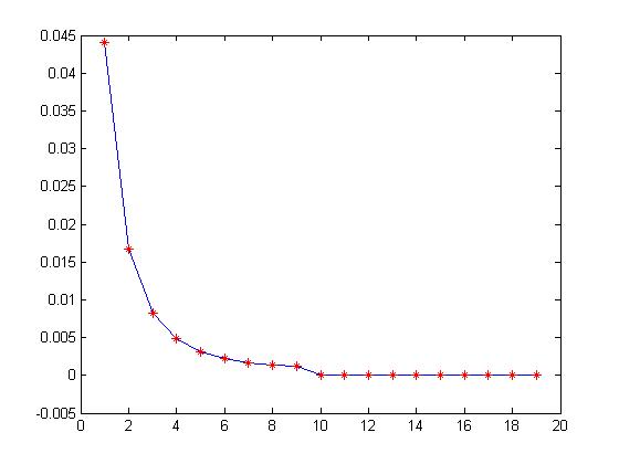
In Fig. 3, we show the reciprocals of the eigenvalues for case $1$ for the permeability field $\kappa_{1}$ and for a particular coarse-grid block. We also show the eigenvalue behavior for both spectral problems. From these figures, we see that the eigenvalues have a very sharp decay for the first $10$ eigenvalues; and this behavior corresponds to the rapid decay in the solution errors shown in Table 1 and Table 3. Starting at the $11$ th eigenvalue, there is no decay any more. This situation signifies that we do not need any additional basis function. In particular, the first $11$ eigenfunctions are enough to achieve a machine precision spectral error, as confirmed in Tables 1 and 3. We observe a very good correlation (0.99) between the error and the eigenvalue behavior.

In order to see the performance of the postprocessing technique discussed in Section 3.4, we repeat the experiments corresponding to Table 1 and compute the postprocessed velocity, denoted as $v_{p}$ . We define $E_{pf}(v)=\|v_{p}-v_{f}\|_{\kappa^{-1},D}/\|v_{f}\|_{\kappa^{-1},D}$ . The numerical results are shown in Table 5. From these results, we clearly see that the postprocessed velocity is much more accurate than the velocity without postprocessing.

Table 5: Comparison of velocity and postprocessed velocity,

\kappa=\kappa_{1}

n=200

and

N=10

	Spectral problem 1		Spectral problem 2
dof per $E$	$E_{of}(v)$	$E_{pf}(v)$	$E_{of}(v)$	$E_{pf}(v)$
1	0.1331	0.1327	0.1523	0.1525
3	0.0569	0.0536	0.0840	0.0823
5	0.0308	0.0232	0.0391	0.0338
7	0.0236	0.0118	0.0278	0.0190
9	0.0210	0.0046	0.0234	0.0114
11	0.0208	0.0037	0.0208	0.0037
20	0.0208	0.0037	0.0208	0.0037

We remark that one can also consider using the curl of the velocity in constructing the offline space. We have studied an offline space construction that uses

a_{i}(v,w)=\int_{\omega_{i}}\text{curl}(\kappa^{-1}v)\text{curl}(\kappa^{-1}w),\quad s_{i}(v,w)=\int_{\omega_{i}}\kappa^{-1}v\cdot w.

(40)

Table 6 shows the convergence of the numerical solution obtained by using this spectral problem. As observed, the numerical results are not as good as those shown earlier for velocity error and for small number of basis functions.

Table 6: Convergence of the offline solution using the curl-based spectral problem,

\kappa=\kappa_{1}

n=200

and

N=10

dof per $E$	$E_{of}(v)$	$E_{of}(p)$	$E_{os}(v)$	$E_{os}(p)$
1	0.1523	0.1018	0.1525	0.0519
3	0.1062	0.0994	0.1052	0.0447
5	0.0996	0.0964	0.0984	0.0373
7	0.0620	0.0902	0.0590	0.0108
9	0.0367	0.0898	0.0305	0.0024
11	0.0312	0.0898	0.0235	0.0013
20	0.0208	0.0898	3.90e-13	5.54e-15

6.2 Oversampling technique

Our first numerical example uses periodic coefficients. Our main objective is to show that oversampling technique can identify the first-order corrector part of the solution and avoid boundary effects. We consider the coefficient

\kappa_{per}(x_{1},x_{2})=\left\{\begin{array}[]{cl}1+\Gamma(x_{1},x_{2})\Pi_{i=1}^{2}(0.4-|x_{i}-0.5|),&\mbox{if $(x_{1},x_{2})\in[0.1,0.9]^{2}$},\\ 1,&\mbox{otherwise},\end{array}\right.

where

\Gamma(x_{1},x_{2})=\frac{2+1.8\sin(2\pi x_{1}/\epsilon)}{2+1.8\sin(2\pi x_{2}/\epsilon)}+\frac{2+1.8\sin(2\pi x_{1}/\epsilon)}{2+1.8\cos(2\pi x_{2}/\epsilon)}.

We consider 4 cases. Case 1. Use oversampling technique to construct the snapshot space. When constructing the snapshot space, we select the eigenvectors corresponding to the first $l_{i}^{+}$ eigenvalues on each coarse edge and use these eigenvectors as our offline space. Case 2. Use oversampling technique to construct the snapshot space. When constructing the snapshot space, we select the eigenvectors corresponding to the first 3 eigenvalues on each coarse edge and perform spectral problem 1 (see Section 3.2) on this snapshot space and select the eigenvectors corresponding to first $l_{i}$ eigenvalues as our offline space. Case 3. Construct the snapshot space without oversampling technique. In this case, we perform spectral problem 1 and select the eigenvectors corresponding to first $l_{i}$ eigenvalues as our offline space. Case 4. Construct the snapshot space without oversampling technique. In this case, we perform spectral problem 2 and select the eigenvectors corresponding to first $l_{i}$ eigenvalues as our offline space. Our numerical results presented in Table 7 show that oversampling technique does give a better performance compared without oversampling, in general. Besides, we can obtain a much smaller snapshot space using oversampling technique while the accuracy of the solution is similar (see cases 2 and 3).

Table 7: Comparison of the 4 cases (relative velocity error w.r.t. fine scale solution),

\kappa=\kappa_{per}

n=200

N=10

dof per $E$	Case 1	Case 2	Case 3	Case 4
1	0.0882	0.0985	0.0987	0.2861
2	0.0241	0.0192	0.0206	0.0214
3	0.0189	0.0189	0.0204	0.0210

Next, we consider the high contrast permeability field $\kappa_{1}$ and compare to the previous results, see Table 8. Again, we see that the error is reduced if we apply oversampling technique and the oversampling allows obtaining a small dimensional snapshot space.

Table 8: Comparison of the 4 cases (relative velocity error w.r.t. fine scale solution),

\kappa=\kappa_{1}

n=200

N=10

dof per $E$	Case 1	Case 2	Case 3	Case 4
1	0.1336	0.1332	0.1331	0.7640
2	0.0400	0.0920	0.0916	0.0991
3	0.0234	0.0234	0.0569	0.0593

6.3 Single-phase flow and transport

We will now consider simulating single-phase flow and transport problems by the mixed GMsFEM with spectral problem 1. Specifically, we consider flow with zero Neumann boundary condition

\begin{split}-\kappa\nabla p&={v},\;\quad\mbox{ in }D,\\ \text{div}\,{v}&=f,\;\quad\mbox{ in }D,\\ v\cdot n&=0,\;\quad\mbox{ on }\partial D.\end{split}

In addition, the saturation equation is given by

S_{t}+v\cdot\nabla S=r,

where $S$ is the saturation and $r$ is the source. The above flow equation is solved by the mixed GMsFEM, and the saturation equation is solved on the fine grid by the finite volume method. Let $S^{n}_{i}$ be the value of $S$ on the fine element $\tau_{i}$ at time $t_{n}$ , where $t_{n}=t_{0}+n\Delta t$ , $t_{0}$ is the initial time and $\Delta t$ is the time step size chosen according to CFL condition. Then, $S^{n}_{i}$ satisfies

|\tau_{i}|\frac{S_{i}^{n+1}-S_{i}^{n}}{\Delta t}+\int_{\partial\tau_{i}}\hat{S}^{n}(v\cdot n)=r_{i}|\tau_{i}|,

(41)

where $r_{i}$ is the average value of $r$ on $\tau_{i}$ and $\hat{S}^{n}$ is the upwind flux.

In our simulations, we will take $f$ to be zero except for the top-left and bottom-right fine-grid elements, where $f$ takes the values of $1$ and $-1$ , respectively. Moreover, we set the initial value of $S$ to be zero. For the source $r$ , we also take it as zero except for the top-left fine element where $r=1$ .

In Figs. 4-7, the saturation plots, shown from left to right, refer to the simulations at different times, namely; $t=1000,3000$ , and $5000$ . The saturation plots in Fig. 4 are obtained by using the fine-scale velocity $v_{f}$ in (41). We denote these saturations $S_{f}$ . Similarly, the saturation plots in Figs. 5-7 are obtained by using the multiscale velocity $v_{o}$ in (41). We denote these saturations $S_{o}$ . When selecting the multiscale basis functions, we use the first spectral problem (10). In order to see the effect of using a different number of multiscale basis functions on each coarse edge, we repeat the simulation with different settings. In the figures, the relative $L^{2}$ error refers to the relative $L^{2}$ error of the saturation. We compute this as

\text{Relative error}=\frac{\|S_{o}-S_{f}\|_{L^{2}(\Omega)}}{\|S_{f}\|_{L^{2}(\Omega)}}.

In addition, we use a $10\times 10$ coarse grid for all simulations.

From Fig. 5, we see that if only one multiscale basis functions are used on each coarse edge, the relative $L^{2}$ error of the saturation is about $4\%$ to $9\%$ . Note that, in this case, the dimension of the velocity space $V^{0}_{\text{off}}$ is only about $0.5\%$ of that of the fine scale velocity space $V^{0}_{h}$ . This shows that the mixed generalized multiscale finite element space has a very good approximation property. We can further reduce the relative error of saturation by using more basis functions per coarse edge. In Figs. 6 and 7, we present the relative errors for saturation when $3$ and $5$ basis functions are used per edge respectively. We see that the errors are reduced to approximately $2\%$ . In these cases, the dimensions of the velocity space $V^{0}_{\text{off}}$ are increased slightly to $1\%$ and $1.4\%$ of the fine scale velocity space $V_{h}^{0}$ , respectively.

6.4 Two-phase flow and transport

Finally, we present our simulation results for two-phase flow and transport problems. Consider the flow problem with zero Neumann boundary condition

\begin{split}-\eta(S)\kappa\nabla p&={v},\;\quad\mbox{ in }D\\ \text{div}\,{v}&=f,\;\quad\mbox{ in }D\\ v\cdot n&=0,\;\quad\mbox{ on }\partial D,\end{split}

where

\eta(S)=\frac{\kappa_{rw}(S)}{\mu_{w}}+\frac{\kappa_{ro}(S)}{\mu_{o}}

and

\kappa_{rw}(S)=S^{2},\;\;\kappa_{ro}(S)=(1-S)^{2},\;\;\mu_{w}=1,\;\;\mu_{o}=5.

The saturation equation is given by

S_{t}+v\cdot\nabla F(S)=r,

where

F(S)=\frac{\kappa_{rw}(S)/\mu_{w}}{\kappa_{rw}(S)/\mu_{w}+\kappa_{ro}(S)/\mu_{o}}.

Adopting the same notations as in the single-phase flow case, we use the following discretization for saturation

|\tau_{i}|\frac{S_{i}^{n+1}-S_{i}^{n}}{\Delta t}+\int_{\partial\tau_{i}}F(\hat{S}^{n})(v\cdot n)=g_{i}|\tau_{i}|.

(42)

The source terms $f$ and $r$ are the same as in the single-phase case. For the construction of the offline space, we also use the spectral problem 1.

In Figs. 8-11, the saturation plots, shown from left to right, refer to the simulations at different times; namely, $t=1000,3000$ , and $5000$ . The saturation plots in Fig. 8 are obtained by using the fine-scale velocity $v_{f}$ in (42). We denote these saturations $S_{f}$ . Similarly, the saturation plots in Figs. 9-11 are obtained by using the multiscale velocity $v_{o}$ in (42). Overall speaking, we observe error reductions from using $1$ basis functions per edge to $5$ basis functions per edge. In particular, for $t=1000$ , the relative error reduces from $9.3\%$ to $2.6\%$ when using $5$ basis functions per edge, and for $t=5000$ , the relative error reduces from $5.5\%$ to $1.3\%$ when using $5$ basis functions per edge.

In our last numerical example, we show the performance of our method when applying to a more realistic permeability field. We pick the top layer of the SPE10 permeability field (see Fig. 2(c)) in the following set of experiments. The model is again the water and oil two-phase flow equations presented above. The permeability field is originally 220 by 60, and we project it into a fine grid of resolution 220 by 220. Then, the coarse grid is set to be 11 by 11, which means the local grid is 10 by 10 in each coarse block. The saturation plots are depicted in Figs. 12-15. In this example, we observe that, at first glance, the multiscale saturation solution looks similar to the fine solution if we use one multiscale basis function per edge. However, if we take a closer look, we notice some missing features in the water front. When we use four or six basis functions per coarse edge, these features can be recovered correctly. This shows the importance of these additional multiscale basis functions. More quantitatively, we observe more error reductions from using $1$ basis functions per edge to $5$ basis functions per edge compared with the previous examples. In particular, for $t=1000$ , the relative error reduces from $18.8\%$ to $3.6\%$ when using $5$ basis functions per edge. Likewise, for $t=5000$ , the relative error reduces from $20.7\%$ to $5.3\%$ when using $5$ basis functions per edge.

7 Conclusions

In this paper, we studied the mixed GMsFEM for constructing a mass conservative solution of the flow equation and investigated applications to two-phase flow and transport. The novelty of our work is in constructing a systematic enrichment for multiscale basis functions for the velocity field. In particular, constructing the snapshot and the offline spaces is one of our novel contributions. We analyze the convergence of the method and give an alternative view of eigenvalue construction. Besides, we study oversampling techniques and construct snapshot vectors as the local solutions in larger regions. The oversampling allows obtaining a much smaller dimensional snapshot space and can help to improve the accuracy of the mixed GMsFEM. Oversampling technique can be particularly helpful for problems with scale separation. We present numerical results and applications to single and two-phase incompressible flow to show the performance of our method.

References

[1] J.E. Aarnes. On the use of a mixed multiscale finite element method for greater flexibility and increased speed or improved accuracy in reservoir simulation. SIAM J. Multiscale Modeling and Simulation, 2:421–439, 2004.
[2] T. Arbogast. Numerical subgrid upscaling of two-phase flow in porous media. In Z. Chen et al., editor, Numerical treatment of multiphase flows in porous media, volume 552, pages 35–49, Berlin, 2000. Springer.
[3] T. Arbogast. Implementation of a locally conservative numerical subgrid upscaling scheme for two-phase Darcy flow. Comput. Geosci., 6:453–481, 2002.
[4] T. Arbogast, G. Pencheva, M.F. Wheeler, and I. Yotov. A multiscale mortar mixed finite element method. SIAM J. Multiscale Modeling and Simulation, 6(1):319–346, 2007.
[5] I. Babuška and R. Lipton. Optimal Local Approximation Spaces for Generalized Finite Element Methods with Application to Multiscale Problems. SIAM Multiscale Modeling and Simulation, 9:373–406, 2011.
[6] F. Brezzi and M. Fortin. Mixed and hybrid finite element methods, volume 15 of Springer Series in Computational Mathematics. Springer-Verlag, New York, 1991.
[7] Z. Chen and T. Y. Hou. A mixed multiscale finite element method for elliptic problems with oscillating coefficients. Mathematics of Computation, 72(242):541–576, 2003.
[8] E. Chung, Y. Efendiev, and G. Li. An adaptive GMsFEM for high contrast flow problems. To appear in J. Comput. Phys.
[9] E. T. Chung and Y. Efendiev. Reduced-contrast approximations for high-contrast multiscale flow problems. Multiscale Model. Simul., 8:1128–1153, 2010.
[10] E. T. Chung, Y. Efendiev, and R. L. Gibson. An energy-conserving discontinuous multiscale finite element method for the wave equation in heterogeneous media. Advances in Adaptive Data Analysis, 3:251–268, 2011.
[11] E. T. Chung and W. T. Leung. A sub-grid structure enhanced discontinuous Galerkin method for multiscale diffusion and convection-diffusion problems. Comm. Comput. Phys., 14:370–392, 2013.
[12] L.J. Durlofsky. Numerical calculation of equivalent grid block permeability tensors for heterogeneous porous media. Water Resour. Res., 27:699–708, 1991.
[13] Y. Efendiev and J. Galvis. A domain decomposition preconditioner for multiscale high-contrast problems. In Y. Huang, R. Kornhuber, O. Widlund, and J. Xu, editors, Domain Decomposition Methods in Science and Engineering XIX, volume 78 of Lecture Notes in Computational Science and Engineering, pages 189–196. Springer-Verlag, 2011.
[14] Y. Efendiev, J. Galvis, and T. Hou. Generalized multiscale finite element methods. J. Comput. Phys., 251:116–135, 2013.
[15] Y. Efendiev, J. Galvis, G. Li, and M. Presho. Generalized multiscale finite element methods. oversampling strategies. IJMM.
[16] Y. Efendiev and T. Hou. Multiscale Finite Element Methods: Theory and Applications, volume 4 of Surveys and Tutorials in the Applied Mathematical Sciences. Springer, New York, 2009.
[17] Y. Efendiev, T. Hou, and X.H. Wu. Convergence of a nonconforming multiscale finite element method. SIAM J. Numer. Anal., 37:888–910, 2000.
[18] R. L. Gibson, K. Gao, E. Chung, and Y. Efendiev. Multiscale modeling of acoustic wave propagation in two-dimensional media. Geophysics, 79:T61–T75, 2014.
[19] T. Hou and X.H. Wu. A multiscale finite element method for elliptic problems in composite materials and porous media. J. Comput. Phys., 134:169–189, 1997.
[20] P. Jenny, S.H. Lee, and H. Tchelepi. Multi-scale finite volume method for elliptic problems in subsurface flow simulation. J. Comput. Phys., 187:47–67, 2003.
[21] X.H. Wu, Y. Efendiev, and T.Y. Hou. Analysis of upscaling absolute permeability. Discrete and Continuous Dynamical Systems, Series B., 2:158–204, 2002.