跳到论文正文
W Papers独立论文阅读器 arXiv:1406.0717 论文正文 计算阅读时间 · 0%
引用这篇论文根据当前论文元数据生成,正式投稿前建议核对。


License: arXiv.org perpetual non-exclusive license
arXiv:1406.0717v1 [math.OC] 03 Jun 2014

Fractional Variational Principle of Herglotz

Ricardo Almeida Email: ricardo.almeida@ua.pt    Agnieszka B. Malinowska Email: a.malinowska@pb.edu.pl
1Department of Mathematics, University of Aveiro, 3810-193 Aveiro, Portugal
3Faculty of Computer Science, Białystok University of Technology,
15-351 Białystok, Poland
Abstract

The aim of this paper is to bring together two approaches to non-conservative systems – the generalized variational principle of Herglotz and the fractional calculus of variations. Namely, we consider functionals whose extrema are sought, by differential equations that involve Caputo fractional derivatives. The Euler–Lagrange equations are obtained for the fractional variational problems of Herglotz-type and the transversality conditions are derived. The fractional Noether-type theorem for conservative and non-conservative physical systems is proved.

Keywords: Calculus of variations, fractional calculus, Caputo fractional derivative, Euler–Lagrange equation, Noether-type theorem.

Mathematics Subject Classification: 49K05; 26A33.

1 Introduction

As it was pointed out by Cornelius Lánczos [15], frictional and non-conservative forces are beyond the usual macroscopic variational treatment and, consequently, beyond the most advanced methods of classical mechanics. Over the years, a number of methods have been presented to circumvent the discrimination against non-conservative systems. We can mention the Rayleigh dissipation function [10]–which is the best known, the Bateman– Caldirola–Kanai (BCK) Lagrangian [18], the generalized variational principle of Herglotz [11, 12] or the fractional calculus of variations [16, 21]. The aim of this paper is to marge the generalized variational principle of Herglotz with the fractional calculus of variations. In other words, we consider functionals whose extrema are sought, by differential equations that involve Caputo fractional derivatives.

The generalized variational principle was proposed by Gustav Herglotz in 1930 (see [12]). It generalizes the classical variational principle by defining the functional through a differential equation. It reduces to the classical variational integral under appropriate conditions. The generalized variational principle gives a variational description of non-conservative processes. For a system, conservative or non-conservative, which can be described with the generalized variational principle, one can systematically derive conserved quantities, as shown in [7, 8, 9], by applying the Noether-type theorem.

The fractional calculus of variations generalizes the classical variational calculus by considering fractional derivatives into the variational integrals to be extremized. Fred Riewe [21] showed that a Lagrangian involving fractional time derivatives leads to an equation of motion with non-conservative forces such as friction. After the seminal papers of Riewe, several different approaches have been developed to generalize the least action principle and the Euler–Lagrange equations to include fractional derivatives. It has been proved, using the notion of Euler–Lagrange fractional extremal, a Noether-type theorem that combines conservative and non-conservative cases of dynamical systems (see [4] or [16] and references given there).

The significance of both approaches to non-conservative systems – the generalized variational principle of Herglotz and the fractional calculus of variations – motivated this work. The paper is organized as follows. In Section 2, for the reader’s convenience, we review the necessary notions of the fractional calculus. Our results are given in next sections: in Section 3 we derive the Euler-–Lagrange equations and the transversality conditions for fractional variational problems of Herglotz-type with one independent variable (Theorems 2 and 3), with higher-order fractional derivatives (Theorems 4 and 5), and for problems with several independent variables (Theorem 6). An heuristic method for solving the Euler–Lagrange equations for the fractional Herglotz-type problem is proposed. Finally, in Section 4 we obtain the fractional Noether-type theorem (Theorem 7 and Theorem 8) that can be used for conservative and non-conservative physical systems. Throughout the paper we illustrate the new results by specific examples.

2 Preliminaries

For the convenience of the reader, we present the definitions of fractional operators that will be used in the sequel. For more on the theory of fractional calculus we refer to [13, 19, 22]; and for general results on the fractional calculus of variations to [16] and references therein.

Let x:[a,b]→ℝx:[a,b]\rightarrow\mathbb{R} be a function, α\alpha be a positive real number and n=[α]+1n=[\alpha]+1, where [α][\alpha] denotes the integer part of α\alpha. In what follows, we assume that xx satisfies appropriate conditions in order to the fractional operators to be well defined. The left and right Riemann–Liouville fractional integrals of order α\alpha are given by

Iαta​x​(t)=1Γ⁡(α)​∫at(t−τ)α−1​x​(τ)​𝑑τ,t>a{{}_{a}I_{t}^{\alpha}}x(t)=\frac{1}{\Gamma(\alpha)}\int_{a}^{t}(t-\tau)^{\alpha-1}x(\tau)d\tau,\quad t>a

and

Iαbt​x​(x)=1Γ⁡(α)​∫tb(τ−t)α−1​x​(τ)​𝑑τ,t<b,{{}_{t}I_{b}^{\alpha}}x(x)=\frac{1}{\Gamma(\alpha)}\int_{t}^{b}(\tau-t)^{\alpha-1}x(\tau)d\tau,\quad t<b,

respectively, where Γ\Gamma represents the Gamma function:

Γ⁡(z)=∫0∞tz−1​e−t​𝑑t.\Gamma(z)=\int_{0}^{\infty}t^{z-1}e^{-t}\,dt.

The left and right Riemann–Liouville fractional derivatives are given by

Dαta​x​(t)=1Γ⁡(n−α)​dnd​tn​∫at(t−τ)n−α−1​x​(τ)​𝑑τ,t>a{{}_{a}D_{t}^{\alpha}}x(t)=\frac{1}{\Gamma(n-\alpha)}\frac{d^{n}}{dt^{n}}\int_{a}^{t}(t-\tau)^{n-\alpha-1}x(\tau)d\tau,\quad t>a

and

Dαbt​x​(t)=(−1)nΓ⁡(n−α)​dnd​tn​∫tb(τ−t)n−α−1​x​(τ)​𝑑τ,t<b,{{}_{t}D_{b}^{\alpha}}x(t)=\frac{(-1)^{n}}{\Gamma(n-\alpha)}\frac{d^{n}}{dt^{n}}\int_{t}^{b}(\tau-t)^{n-\alpha-1}x(\tau)d\tau,\quad t<b,

respectively. The left and right Caputo fractional derivatives are defined by

DtαaC​x​(t)=1Γ⁡(n−α)​∫at(t−τ)n−α−1​x(n)​(τ)​𝑑τ,t>a{{}^{C}_{a}D_{t}^{\alpha}}x(t)=\frac{1}{\Gamma(n-\alpha)}\int_{a}^{t}(t-\tau)^{n-\alpha-1}x^{(n)}(\tau)d\tau,\quad t>a

and

DbαtC​x​(t)=(−1)nΓ⁡(n−α)​∫tb(τ−t)n−α−1​x(n)​(τ)​𝑑τ,t<b,{{}^{C}_{t}D_{b}^{\alpha}}x(t)=\frac{(-1)^{n}}{\Gamma(n-\alpha)}\int_{t}^{b}(\tau-t)^{n-\alpha-1}x^{(n)}(\tau)d\tau,\quad t<b,

respectively. The integration by parts formula plays a crucial role in deriving the Euler–Lagrange equation. For the left Caputo fractional derivative, this formula is formulated the following way.

Theorem 1.

([14])) Let α>0\alpha>0, and x,y:[a,b]→ℝx,y:[a,b]\to\mathbb{R} be two functions of class CnC^{n}, with n=[α]+1n=[\alpha]+1. Then,

∫aby⁡(t)⋅DtαaC​x​(t)​𝑑t=∫abx⁡(t)⋅Dαbt​y​(t)​𝑑t+∑j=0n−1[Dα+j−nbt​y​(t)⋅(−1)n−1−j​x(n−1−j)​(t)]ab.\int_{a}^{b}y(t)\cdot{{}_{a}^{C}D_{t}^{\alpha}}x(t)dt=\int_{a}^{b}x(t)\cdot{{}_{t}D_{b}^{\alpha}}y(t)dt+\sum_{j=0}^{n-1}\left[{{}_{t}D_{b}^{\alpha+j-n}}y(t)\cdot(-1)^{n-1-j}x^{(n-1-j)}(t)\right]_{a}^{b}.

Partial fractional integrals and derivatives for functions of pp independent variables are defined in a similar way as is done for integer order derivatives. Let x:∏i=1p[ai,bi]→ℝx:\prod_{i=1}^{p}[a_{i},b_{i}]\to\mathbb{R} be a function, αi\alpha_{i}, i=1,…,pi=1,\ldots,p be real numbers and define ni=[αi]+1n_{i}=[\alpha_{i}]+1. Then, we define the partial Riemann–Liouville fractional integrals of order αi\alpha_{i} with respect to tit_{i} by

Iαitiai​x​(t1,…,tp)=1Γ⁡(αi)​∫aiti(ti−τi)αi−1​x​(t1,…,ti−1,τi,ti+1,…,tp)​d​τi,{{}_{a_{i}}I_{t_{i}}^{{\alpha}_{i}}}x(t_{1},\ldots,t_{p})=\frac{1}{\Gamma(\alpha_{i})}\int_{a_{i}}^{t_{i}}(t_{i}-\tau_{i})^{\alpha_{i}-1}x(t_{1},\ldots,t_{i-1},\tau_{i},t_{i+1},\ldots,t_{p})d\tau_{i},
Iαibiti​x​(t1,…,tp)=1Γ⁡(αi)​∫tibi(τi−ti)αi−1​x​(t1,…,ti−1,τi,ti+1,…,tp)​d​τi.{{}_{t_{i}}I_{b_{i}}^{{\alpha}_{i}}}x(t_{1},\ldots,t_{p})=\frac{1}{\Gamma(\alpha_{i})}\int_{t_{i}}^{b_{i}}(\tau_{i}-t_{i})^{\alpha_{i}-1}x(t_{1},\ldots,t_{i-1},\tau_{i},t_{i+1},\ldots,t_{p})d\tau_{i}.

Partial Riemann–Liouville and Caputo derivatives are defined by

Dαitiai​x​(t1,…,tp)=1Γ⁡(ni−αi)​∂ni∂tini​∫aiti(ti−τi)ni−αi−1​x​(t1,…,ti−1,τi,ti+1,…,tp)​d​τi,{{}_{a_{i}}D_{t_{i}}^{{\alpha}_{i}}}x(t_{1},\ldots,t_{p})=\frac{1}{\Gamma(n_{i}-\alpha_{i})}\frac{\partial^{n_{i}}}{\partial t_{i}^{n_{i}}}\int_{a_{i}}^{t_{i}}(t_{i}-\tau_{i})^{n_{i}-\alpha_{i}-1}x(t_{1},\ldots,t_{i-1},\tau_{i},t_{i+1},\ldots,t_{p})d\tau_{i},
Dαibiti​x​(t1,…,tp)=(−1)niΓ⁡(ni−αi)​∂ni∂tini​∫tibi(τi−ti)ni−αi−1​x​(t1,…,ti−1,τi,ti+1,…,tp)​d​τi,{{}_{t_{i}}D_{b_{i}}^{{\alpha}_{i}}}x(t_{1},\ldots,t_{p})=\frac{(-1)^{n_{i}}}{\Gamma(n_{i}-\alpha_{i})}\frac{\partial^{n_{i}}}{\partial t_{i}^{n_{i}}}\int_{t_{i}}^{b_{i}}(\tau_{i}-t_{i})^{n_{i}-\alpha_{i}-1}x(t_{1},\ldots,t_{i-1},\tau_{i},t_{i+1},\ldots,t_{p})d\tau_{i},
DtiαiaiC​x​(t1,…,tp)=1Γ⁡(ni−αi)​∫aiti(ti−τi)ni−αi−1​∂ni∂tini​x​(t1,…,ti−1,τi,ti+1,…,tp)​d​τi,{{}^{C}_{a_{i}}D_{t_{i}}^{\alpha_{i}}}x(t_{1},\ldots,t_{p})=\frac{1}{\Gamma(n_{i}-\alpha_{i})}\int_{a_{i}}^{t_{i}}(t_{i}-\tau_{i})^{n_{i}-\alpha_{i}-1}\frac{\partial^{n_{i}}}{\partial t_{i}^{n_{i}}}x(t_{1},\ldots,t_{i-1},\tau_{i},t_{i+1},\ldots,t_{p})d\tau_{i},
DbiαitiC​x​(t1,…,tp)=(−1)niΓ⁡(ni−αi)​∫tibi(τi−ti)ni−αi−1​∂ni∂tini​x​(t1,…,ti−1,τi,ti+1,…,tp)​d​τi.{{}^{C}_{t_{i}}D_{b_{i}}^{\alpha_{i}}}x(t_{1},\ldots,t_{p})=\frac{(-1)^{n_{i}}}{\Gamma(n_{i}-\alpha_{i})}\int_{t_{i}}^{b_{i}}(\tau_{i}-t_{i})^{n_{i}-\alpha_{i}-1}\frac{\partial^{n_{i}}}{\partial t_{i}^{n_{i}}}x(t_{1},\ldots,t_{i-1},\tau_{i},t_{i+1},\ldots,t_{p})d\tau_{i}.

3 The generalized fractional Euler–Lagrange equations

Consider the differential equation with dependence on Caputo fractional derivatives

d​zd​t=L⁡(t,x⁡(t),DtαaC​x​(t),z⁡(t)),t∈[a,b],\frac{dz}{dt}=L(t,x(t),{{}^{C}_{a}D^{\alpha}_{t}}x(t),z(t)),\quad t\in[a,b], (1)

with the initial condition z⁡(a)=zaz(a)=z_{a}, where tt is the independent variable, x=(x1,…,xn)x=(x_{1},\ldots,x_{n}) the dependent variable and

DtαaC​x​(t):=(Dtα1aC​x1​(t),…,DtαnaC​xn​(t)).{{}^{C}_{a}D^{\alpha}_{t}}x(t):=({{}^{C}_{a}D^{\alpha_{1}}_{t}}x_{1}(t),\ldots,{{}^{C}_{a}D^{\alpha_{n}}_{t}}x_{n}(t)).

In what follows we assume that:

  1. 1.

    x⁡(a)=xax(a)=x_{a}, x⁡(b)=xbx(b)=x_{b}, xa,xb∈ℝnx_{a},x_{b}\in\mathbb{R}^{n};

  2. 2.

    αj∈(0,1)\alpha_{j}\in(0,1), j=1,…,nj=1,\ldots,n;

  3. 3.

    x∈C1​([a,b],ℝn)x\in C^{1}([a,b],\mathbb{R}^{n}), DtαaC​x∈C1​([a,b],ℝn){{}^{C}_{a}D^{\alpha}_{t}}x\in C^{1}([a,b],\mathbb{R}^{n});

  4. 4.

    the Lagrangian L:[a,b]×ℝ2​n+1→ℝL:[a,b]\times\mathbb{R}^{2n+1}\to\mathbb{R} is of class C1C^{1} and the maps t↦λ⁡(t)​∂L∂DtαjaC​xj​[x,z]​(t)t\mapsto\displaystyle\lambda(t)\frac{\partial L}{\partial{{}^{C}_{a}D^{\alpha_{j}}_{t}}x_{j}}[x,z](t) are such that Dbαjt​(λ⁡(t)​∂L∂DtαjaC​xj​[x,z]​(t))\displaystyle{{}_{t}D^{\alpha_{j}}_{b}\left(\lambda(t)\frac{\partial L}{\partial{{}^{C}_{a}D^{\alpha_{j}}_{t}}x_{j}}[x,z](t)\right)}, j=1,…,nj=1,\ldots,n, exist and are continuous on [a,b][a,b], where

    [x,z](t):=(t,x(t),DtαaCx(t),z(t))andλ(t):=exp(−∫at∂L∂z[x,z](τ)dτ).[x,z](t):=(t,x(t),{{}^{C}_{a}D^{\alpha}_{t}}x(t),z(t))\quad\mbox{and}\quad\lambda(t):=\exp\left(-\int_{a}^{t}\frac{\partial L}{\partial z}[x,z](\tau)d\tau\right).

For any arbitrary but fixed function x⁡(t)x(t) and a fixed initial value z⁡(a)=zaz(a)=z_{a} the solution of the differential equation (1): z⁡[x;t]=z⁡(t,x⁡(t),DtαaC​x​(t))z[x;t]=z(t,x(t),{{}^{C}_{a}D^{\alpha}_{t}}x(t)) exists, and depends on tt, x⁡(t)x(t) and DtαaC​x​(t){{}^{C}_{a}D^{\alpha}_{t}}x(t) (see, e.g., [1]). Moreover, under our assumptions, is a C2C^{2} function of its arguments. In order for the equation (1) to define a functional, zz, of x⁡(t)x(t) we must solve equation (1) with the same fixed initial condition z⁡(a)=zaz(a)=z_{a} for all argument functions x⁡(t)x(t), and evaluate the solution z=z⁡[x;t]z=z[x;t] at the same fixed final time t=bt=b for all argument functions x⁡(t)x(t).

The fractional variational principle of Herglotz (FVPH) is as follows:
Let the functional z=z⁡[x;b]z=z[x;b] of x⁡(t)x(t) be given by a differential equation of the form (1) and let the function η∈C1​([a,b],ℝn)\eta\in C^{1}([a,b],\mathbb{R}^{n}) satisfies the boundary conditions η⁡(a)=η⁡(b)=0\eta(a)=\eta(b)=0 and such that DtαaC​η∈C1​([a,b],ℝn){{}^{C}_{a}D^{\alpha}_{t}}\eta\in C^{1}([a,b],\mathbb{R}^{n}). Then the value of the functional z⁡[x;b]z[x;b] is an extremum for function x⁡(t)x(t) which satisfy the condition

dd​ϵ​z​[x+ϵ​η;b]|ϵ=0=dd​ϵ​z​(b,x⁡(b)+ϵ​η​(b),DbαaC​x​(b)+ϵ​DbαaC​η​(b))|ϵ=0=0.\frac{d}{d\epsilon}\left.z[x+\epsilon\eta;b]\right|_{\epsilon=0}=\frac{d}{d\epsilon}\left.z\left(b,x(b)+\epsilon\eta(b),{{}^{C}_{a}D^{\alpha}_{b}}x(b)+\epsilon{{}^{C}_{a}D^{\alpha}_{b}}\eta(b)\right)\right|_{\epsilon=0}=0. (2)

Observe that, if we introduce a parameter ϵ\epsilon in the equation (1), then the solution zz still exists and depends also on ϵ\epsilon, and it is differentiable with respect to ϵ\epsilon (see, e.g., Section 2.6 in [1]). Moreover, under our assumptions, zz is a C2C^{2} function of its arguments.

Remark 1.

Later we will consider the case where x⁡(b)x(b) is free and deduce the respective natural boundary conditions. In this case, the functions η\eta that we consider in the formulation of the (FVPH) are such that η⁡(a)=0\eta(a)=0 but η⁡(b)\eta(b) may take any value.

Remark 2.

In the case when α→1\alpha\to 1, FVPH gives the classical variational principle of Herglotz (see [12]).

Remark 3.

In the fractional calculus of variations, LL does not depend on zz and we can integrated from aa to bb, to obtain the functional

z⁡[x]=∫ab[L⁡(t,x⁡(t),DtαaC​x​(t))+zab−a]​𝑑t.z[x]=\int_{a}^{b}\left[L(t,x(t),{{}^{C}_{a}D^{\alpha}_{t}}x(t))+\frac{z_{a}}{b-a}\right]dt.
Theorem 2.

Let x=(x1,…,xn)x=(x_{1},\ldots,x_{n}) be such that z⁡[x;b]z[x;b] defined by equation (1) attains an extremum. Then xx is a solution of

λ(t)∂L∂xj[x,z](t)+Dbαjt(λ(t)∂L∂DtαjaC​xj[x,z](t))=0,j=1,…n\lambda(t)\frac{\partial L}{\partial x_{j}}[x,z](t)+{{}_{t}D^{\alpha_{j}}_{b}\left(\lambda(t)\frac{\partial L}{\partial{{}^{C}_{a}D^{\alpha_{j}}_{t}}x_{j}}[x,z](t)\right)}=0,\quad j=1,\ldots n (3)

on [a,b][a,b].

Proof.

Let xx be such that z⁡[x;b]z[x;b] defined by equation (1) attains an extremum. We will show that (3) is a consequence of condition (2). The rate of change of zz, in the direction of η\eta, is given by

θ⁡(t)=dd​ϵ​z​[x+ϵ​η;t]|ϵ=0=dd​ϵ​z​(t,x⁡(t)+ϵ​η​(t),DtαaC​x​(t)+ϵ​DtαaC​η​(t))|ϵ=0.\theta(t)=\frac{d}{d\epsilon}\left.z[x+\epsilon\eta;t]\right|_{\epsilon=0}=\frac{d}{d\epsilon}\left.z\left(t,x(t)+\epsilon\eta(t),{{}^{C}_{a}D^{\alpha}_{t}}x(t)+\epsilon{{}^{C}_{a}D^{\alpha}_{t}}\eta(t)\right)\right|_{\epsilon=0}. (4)

Applying the variation ϵ​η\epsilon\eta to the argument function in equation (1) we get

dd​t​z​[x+ϵ​η;t]=L⁡(t,x⁡(t)+ϵ​η​(t),DtαaC​x​(t)+ϵ​DtαaC​η​(t),z⁡[x+ϵ​η;t]).\frac{d}{dt}z[x+\epsilon\eta;t]=L(t,x(t)+\epsilon\eta(t),{{}^{C}_{a}D^{\alpha}_{t}}x(t)+\epsilon{{}^{C}_{a}D^{\alpha}_{t}}\eta(t),z[x+\epsilon\eta;t]).

Observe that,

θ˙​(t)=dd​t​θ​(t)=dd​t​dd​ϵ​z​(t,x⁡(t)+ϵ​η​(t),DtαaC​x​(t)+ϵ​DtαaC​η​(t))|ϵ=0=dd​ϵ​dd​t​z​(t,x⁡(t)+ϵ​η​(t),DtαaC​x​(t)+ϵ​DtαaC​η​(t))|ϵ=0=dd​ϵ​L​(t,x⁡(t)+ϵ​η​(t),DtαaC​x​(t)+ϵ​DtαaC​η​(t),z⁡[x+ϵ​η;t])|ϵ=0.\dot{\theta}(t)=\frac{d}{dt}\theta(t)=\frac{d}{dt}\frac{d}{d\epsilon}\left.z\left(t,x(t)+\epsilon\eta(t),{{}^{C}_{a}D^{\alpha}_{t}}x(t)+\epsilon{{}^{C}_{a}D^{\alpha}_{t}}\eta(t)\right)\right|_{\epsilon=0}\\ =\frac{d}{d\epsilon}\frac{d}{dt}\left.z\left(t,x(t)+\epsilon\eta(t),{{}^{C}_{a}D^{\alpha}_{t}}x(t)+\epsilon{{}^{C}_{a}D^{\alpha}_{t}}\eta(t)\right)\right|_{\epsilon=0}\\ =\left.\frac{d}{d\epsilon}L\left(t,x(t)+\epsilon\eta(t),{{}^{C}_{a}D^{\alpha}_{t}}x(t)+\epsilon{{}^{C}_{a}D^{\alpha}_{t}}\eta(t),z[x+\epsilon\eta;t]\right)\right|_{\epsilon=0}.

This gives a differential equation for θ⁡(t)\theta(t):

θ˙​(t)−∂L∂z​[x,z]​(t)​θ​(t)=∑j=1n(∂L∂xj​[x,z]​(t)​ηj​(t)+∂L∂DtαjaC​xj​[x,z]​(t)​DtαjaC​ηj​(t))\dot{\theta}(t)-\frac{\partial L}{\partial z}[x,z](t)\theta(t)=\sum_{j=1}^{n}\left(\frac{\partial L}{\partial x_{j}}[x,z](t)\eta_{j}(t)+\frac{\partial L}{\partial{{}^{C}_{a}D^{\alpha_{j}}_{t}}x_{j}}[x,z](t){{}^{C}_{a}D^{\alpha_{j}}_{t}}\eta_{j}(t)\right)

whose solution is

θ⁡(t)​λ​(t)−θ⁡(a)=∫at∑j=1n(∂L∂xj​[x,z]​(τ)​ηj​(τ)+∂L∂DταjaC​xj​[x,z]​(τ)​DταjaC​ηj​(t))​λ​(τ)​𝑑τ\theta(t)\lambda(t)-\theta(a)=\int_{a}^{t}\sum_{j=1}^{n}\left(\frac{\partial L}{\partial x_{j}}[x,z](\tau)\eta_{j}(\tau)+\frac{\partial L}{\partial{{}^{C}_{a}D^{\alpha_{j}}_{\tau}}x_{j}}[x,z](\tau){{}^{C}_{a}D^{\alpha_{j}}_{\tau}}\eta_{j}(t)\right)\lambda(\tau)d\tau

with notation λ(t)=exp(−∫at∂L∂z[x,z](τ)dτ)\lambda(t)=\exp\left(-\int_{a}^{t}\frac{\partial L}{\partial z}[x,z](\tau)d\tau\right). Observe that θ⁡(a)=0\theta(a)=0. Indeed, as explained earlier, we evaluate the solution of the equation (1) with the same fixed initial condition z⁡(a)z(a), independently of the function x⁡(t)x(t). At t=bt=b, we get

θ⁡(b)​λ​(b)=∫ab∑j=1n(∂L∂xj​[x,z]​(t)​ηj​(t)+∂L∂DtαjaC​xj​[x,z]​(t)​DtαjaC​ηj​(t))​λ​(t)​𝑑t\theta(b)\lambda(b)=\int_{a}^{b}\sum_{j=1}^{n}\left(\frac{\partial L}{\partial x_{j}}[x,z](t)\eta_{j}(t)+\frac{\partial L}{\partial{{}^{C}_{a}D^{\alpha_{j}}_{t}}x_{j}}[x,z](t){{}^{C}_{a}D^{\alpha_{j}}_{t}}\eta_{j}(t)\right)\lambda(t)dt

Observe that θ⁡(b)\theta(b) is the variation of z⁡[x;b]z[x;b]. If xx is such that z⁡[x;b]z[x;b] defined by equation (1) attains an extremum, then θ⁡(b)\theta(b) is identically zero. Hence, we get

∫abλ⁡(t)​∑j=1n(∂L∂xj​[x,z]​(t)​ηj​(t)+∂L∂DtαjaC​xj​[x,z]​(t)​DtαjaC​ηj​(t))​𝑑t=0.\int_{a}^{b}\lambda(t)\sum_{j=1}^{n}\left(\frac{\partial L}{\partial x_{j}}[x,z](t)\eta_{j}(t)+\frac{\partial L}{\partial{{}^{C}_{a}D^{\alpha_{j}}_{t}}x_{j}}[x,z](t){{}^{C}_{a}D^{\alpha_{j}}_{t}}\eta_{j}(t)\right)dt=0.

Integrating by parts (cf. Theorem 1) we get

∫ab∑j=1n[λ⁡(t)​∂L∂xj​[x,z]​(t)+Dbαjt​(λ⁡(t)​∂L∂DtαjaC​xj​[x,z]​(t))]​ηj​(t)​𝑑t+∑j=1n[ηj(t)tI1−αjb(λ(t)∂L∂DtαjaC​xj[x,z](t))]ab=0.\int_{a}^{b}\sum_{j=1}^{n}\left[\lambda(t)\frac{\partial L}{\partial x}_{j}[x,z](t)+{{}_{t}D^{\alpha_{j}}_{b}}\left(\lambda(t)\frac{\partial L}{\partial{{}^{C}_{a}D^{\alpha_{j}}_{t}}x_{j}}[x,z](t)\right)\right]\eta_{j}(t)dt\\ +\sum_{j=1}^{n}\left[\eta_{j}(t){{}_{t}I^{1-\alpha_{j}}_{b}}\left(\lambda(t)\frac{\partial L}{\partial{{}^{C}_{a}D^{\alpha_{j}}_{t}}x_{j}}[x,z](t)\right)\right]_{a}^{b}=0.

Since η⁡(a)=η⁡(b)=0\eta(a)=\eta(b)=0, and η\eta is an arbitrary function elsewhere, equation (3) follows by the fundamental lemma of the calculus of variations. ∎

Remark 4.

The function θ\theta in Eq. (4) is well defined (see, e.g., Section 2.6 in [1]).

Remark 5.

Let αj\alpha_{j} goes to 11, for all j=1,…,nj=1,\ldots,n and the Lagrangian LL is of the C2C^{2} class. Then equations (3) become

λ(t)∂L∂xj[x,z](t)−dd​t(λ(t)∂L∂x˙j[x,z](t))=0,j=1,…,n.\lambda(t)\frac{\partial L}{\partial x_{j}}[x,z](t)-\frac{d}{dt}\left(\lambda(t)\frac{\partial L}{\partial\dot{x}_{j}}[x,z](t)\right)=0,\quad j=1,\ldots,n.

Then, since λ˙​(t)=−∂L∂z​[x,z]​(t)​λ​(t)\dot{\lambda}(t)=\displaystyle-\frac{\partial L}{\partial z}[x,z](t)\lambda(t), we get

λ⁡(t)​[∂L∂xj​[x,z]​(t)+∂L∂z​[x,z]​(t)​∂L∂x˙j​[x,z]​(t)−dd​t​∂L∂x˙j​[x,z]​(t)]=0\lambda(t)\left[\frac{\partial L}{\partial x_{j}}[x,z](t)+\frac{\partial L}{\partial z}[x,z](t)\frac{\partial L}{\partial\dot{x}_{j}}[x,z](t)-\frac{d}{dt}\frac{\partial L}{\partial\dot{x}_{j}}[x,z](t)\right]=0

if and only if

∂L∂xj[x,z](t)+∂L∂z[x,z](t)∂L∂x˙j[x,z](t)−dd​t∂L∂x˙j[x,z](t)=0,j=1,…,n.\frac{\partial L}{\partial x_{j}}[x,z](t)+\frac{\partial L}{\partial z}[x,z](t)\frac{\partial L}{\partial\dot{x}_{j}}[x,z](t)-\frac{d}{dt}\frac{\partial L}{\partial\dot{x}_{j}}[x,z](t)=0,\quad j=1,\ldots,n. (5)

To equations (5), Herglotz called the generalized Euler–Lagrange equations [12].

Example 1.

Consider the system

{z˙(t)=[C0D0.5tx(t)−2Γ⁡(2.5)t1.5]2, with t∈[0,1],z⁡(0)=0,x(0)=0,x(1)=1.\left\{\begin{array}[]{l}\dot{z}(t)=\left[{{}^{C}_{0}D^{0.5}_{t}}x(t)-\frac{2}{\Gamma(2.5)}t^{1.5}\right]^{2},\quad\mbox{ with }\,t\in[0,1],\\ z(0)=0,\\ x(0)=0,\,x(1)=1.\end{array}\right.

We wish to find a curve xx for which z⁡[x;1]z[x;1] attains the minimum value. Observe that for all xx, we have that zz is an increasing function and thus z⁡(t)≥0z(t)\geq 0, for all t∈[0,1]t\in[0,1].

Let x¯​(t)=t2\overline{x}(t)=t^{2}. Then Dt0.50C​x¯​(t)=2Γ⁡(2.5)​t1.5{{}^{C}_{0}D^{0.5}_{t}}\overline{x}(t)=\frac{2}{\Gamma(2.5)}t^{1.5} (see e.g. [13]). For such choice of xx we get the differential equation z˙​(t)=0\dot{z}(t)=0. As z⁡(0)=0z(0)=0 the unique solution is z¯​(t)=0\overline{z}(t)=0. Therefore z⁡[x;1]z[x;1] obtain the minimum value, which is 00, at x¯\overline{x}. In this case λ⁡(t)=1\lambda(t)=1 and equation (3) takes the form

D0.51t​[Dt0.50C​x​(t)−2Γ⁡(2.5)​t1.5]=0{{}_{t}D_{1}^{0.5}}\left[{{}^{C}_{0}D^{0.5}_{t}}x(t)-\frac{2}{\Gamma(2.5)}t^{1.5}\right]=0

which is satisfied for x¯\overline{x}.

Example 2.

Consider the system with the Lagrangian depending on zz:

{z˙(t)=[C0D0.5tx(t)−2Γ⁡(2.5)t1.5]2exp(t)+z, with t∈[0,1],z⁡(0)=1,x(0)=0,x(1)=1.\left\{\begin{array}[]{l}\dot{z}(t)=\left[{{}^{C}_{0}D^{0.5}_{t}}x(t)-\frac{2}{\Gamma(2.5)}t^{1.5}\right]^{2}\exp(t)+z,\quad\mbox{ with }\,t\in[0,1],\\ z(0)=1,\\ x(0)=0,\,x(1)=1.\\ \end{array}\right.

In this case we have λ⁡(t)=exp⁡(−t)\lambda(t)=\exp(-t) and equation (3) takes the form

D0.51t​[exp⁡(−t)​(Dt0.50C​x​(t)−2Γ⁡(2.5)​t1.5)​exp⁡(t)]=0.{{}_{t}D_{1}^{0.5}}\left[\exp(-t)\left({{}^{C}_{0}D^{0.5}_{t}}x(t)-\frac{2}{\Gamma(2.5)}t^{1.5}\right)\exp(t)\right]=0. (6)

Observe that the function x¯​(t)=t2\overline{x}(t)=t^{2} is a solution to equation (6), but we cannot conclude that it is a minimizer (or maximizer) of the functional z⁡[x;1]z[x;1].

Note that in order to uniquely determine the unknown function xx which is a solution to equation (3), we must consider the system of differential equations

{d​zd​t=L​[x,z]​(t),λ⁡(t)​∂L∂xj​[x,z]​(t)+Dbαjt​(λ⁡(t)​∂L∂DtαjaC​xj​[x,z]​(t))=0,\left\{\begin{array}[]{l}\displaystyle\frac{dz}{dt}=L[x,z](t),\\ \displaystyle\lambda(t)\frac{\partial L}{\partial x_{j}}[x,z](t)+{{}_{t}D^{\alpha_{j}}_{b}\left(\lambda(t)\frac{\partial L}{\partial{{}^{C}_{a}D^{\alpha_{j}}_{t}}x_{j}}[x,z](t)\right)}=0,\end{array}\right.

with λ(t)=exp(−∫at∂L∂z[x,z](τ)dτ)\lambda(t)=\exp\left(-\int_{a}^{t}\frac{\partial L}{\partial z}[x,z](\tau)d\tau\right) together with the boundary condition: z⁡(a)=zaz(a)=z_{a}, x⁡(a)=xax(a)=x_{a}, x⁡(b)=xbx(b)=x_{b}, where za∈ℝz_{a}\in\mathbb{R} and xa,xb∈ℝnx_{a},x_{b}\in\mathbb{R}^{n}. In the case where xj​(b)x_{j}(b), j∈{1,…,n}j\in\{1,\ldots,n\}, is not specified we need an additional condition known as the transversality condition.

Theorem 3.

Let xx be such that z⁡[x;b]z[x;b] defined by equation (1) attains an extremum. Then, xx is a solution to the system of fractional differential equations (3). If xj​(b)x_{j}(b), j∈{1,…,n}j\in\{1,\ldots,n\}, is not specified, then the transversality condition

Ib1−αjt​(λ⁡(t)​∂L∂DtαjaC​xj​[x,z]​(t))=0att=b{{}_{t}I^{1-\alpha_{j}}_{b}}\left(\lambda(t)\frac{\partial L}{\partial{{}^{C}_{a}D^{\alpha_{j}}_{t}}x_{j}}[x,z](t)\right)=0\quad\mbox{at}\quad t=b (7)

holds.

Proof.

The only difference with respect to the proof of Theorem 2 is that ηj​(b)\eta_{j}(b) may vanish or not. Assuming first that ηj​(b)=0\eta_{j}(b)=0 we deduce equations (3). Therefore

∑j=1n[ηj​(t)​Ib1−αjt​(λ⁡(t)​∂L∂DtαjaC​xj​[x,z]​(t))]ab=0.\sum_{j=1}^{n}\left[\eta_{j}(t){{}_{t}I^{1-\alpha_{j}}_{b}}\left(\lambda(t)\frac{\partial L}{\partial{{}^{C}_{a}D^{\alpha_{j}}_{t}}x_{j}}[x,z](t)\right)\right]_{a}^{b}=0.

Since η⁡(a)=0\eta(a)=0, ηi​(b)=0\eta_{i}(b)=0 for i≠ji\neq j and ηj​(b)\eta_{j}(b) is arbitrary equation (7) follows. ∎

When dealing with fractional operators usually we do not need to assume that functions have a nice behavior in the sense of smoothness properties. From the other hand, the drawback is that equations of type (3) are in most cases impossible to be solved analytically, and to overcome this problem numerical methods are applied (see, e.g., [3, 5, 6, 20]). One of these methods consists in replacing the fractional operator by an expansion that involves only integer order derivatives [22]. Let α∈(0,1)\alpha\in(0,1), (c,d)(c,d) be an open interval in ℝ\mathbb{R}, and [a,b]⊂(c,d)[a,b]\subset(c,d) be such that for each t∈[a,b]t\in[a,b] the closed ball Bb−a​(t)B_{b-a}(t), with center at tt and radius b−ab-a, lies in (c,d)(c,d). If xx is an analytic function in (c,d)(c,d) then

Dαta​x​(t)=∑k=0∞(αk)​(t−a)k−αΓ⁡(k+1−α)​x(k)​(t), where ​(αk)=(−1)k−1​α​Γ​(k−α)Γ⁡(1−α)​Γ​(k+1).{{}_{a}D_{t}^{\alpha}}x(t)=\sum_{k=0}^{\infty}\binom{\alpha}{k}\frac{(t-a)^{k-\alpha}}{\Gamma(k+1-\alpha)}x^{(k)}(t),\quad\text{ where }\binom{\alpha}{k}=\frac{(-1)^{k-1}\alpha\Gamma(k-\alpha)}{\Gamma(1-\alpha)\Gamma(k+1)}. (8)

Using the well-known relations between the two type of fractional derivatives,

DtαaC​x​(t)=Dαta​x​(t)−x⁡(a)Γ⁡(1−α)​(t−a)−α,{{}_{a}^{C}D_{t}^{\alpha}}x(t)={{}_{a}D_{t}^{\alpha}}x(t)-\frac{x(a)}{\Gamma(1-\alpha)}(t-a)^{-\alpha}, (9)

similar formula is given for the Caputo fractional derivative.
For simplicity, let us assume that n=1n=1 and fix N∈ℕN\in\mathbb{N}. If x∈C2​N​([a,b],ℝ)x\in C^{2N}([a,b],\mathbb{R}), L∈CN+1​([a,b]×ℝ3,ℝ)L\in C^{N+1}([a,b]\times\mathbb{R}^{3},\mathbb{R}), then by replacing the fractional derivative in equation (1) by formulas (8)–(9), with the approximation up to order NN, we obtain

z˙​(t)=L⁡(t,x⁡(t),∑k=0N(αk)​(t−a)k−αΓ⁡(k+1−α)​x(k)​(t)−xaΓ⁡(1−α)​(t−a)−α,z⁡(t))\dot{z}(t)=L\left(t,x(t),\sum_{k=0}^{N}\binom{\alpha}{k}\frac{(t-a)^{k-\alpha}}{\Gamma(k+1-\alpha)}x^{(k)}(t)-\frac{x_{a}}{\Gamma(1-\alpha)}(t-a)^{-\alpha},z(t)\right)

with t∈[a,b]t\in[a,b]. Define

L¯​(t,x⁡(t),x˙​(t),…,x(N)​(t),z⁡(t))\overline{L}(t,x(t),\dot{x}(t),\ldots,x^{(N)}(t),z(t))
:=L⁡(t,x⁡(t),∑k=0N(αk)​(t−a)k−αΓ⁡(k+1−α)​x(k)​(t)−xaΓ⁡(1−α)​(t−a)−α,z⁡(t)).:=L\left(t,x(t),\sum_{k=0}^{N}\binom{\alpha}{k}\frac{(t-a)^{k-\alpha}}{\Gamma(k+1-\alpha)}x^{(k)}(t)-\frac{x_{a}}{\Gamma(1-\alpha)}(t-a)^{-\alpha},z(t)\right).

Therefore, we got the higher-order variational problems of Herglotz (see [23])

z˙​(t)=L¯​(t,x⁡(t),x˙​(t),…,x(N)​(t),z⁡(t)), with ​t∈[a,b].\dot{z}(t)=\overline{L}(t,x(t),\dot{x}(t),\ldots,x^{(N)}(t),z(t)),\quad\mbox{ with }\,t\in[a,b].

As it was proved in [23], if xNx_{N} is such that zN​[xN;b]z_{N}[x_{N};b] attains an extremum, then (xN,zN)(x_{N},z_{N}) satisfies the Euler–Lagrange equation

∑k=0N(−1)k​dkd​tk​(λN​(t)​∂L¯∂x(k)​(t,x⁡(t),x˙​(t),…,x(N)​(t),z⁡(t)))=0,\sum_{k=0}^{N}(-1)^{k}\frac{d^{k}}{dt^{k}}\left(\lambda_{N}(t)\frac{\partial\overline{L}}{\partial x^{(k)}}(t,x(t),\dot{x}(t),\ldots,x^{(N)}(t),z(t))\right)=0,

on [a,b][a,b], where λN(t)=exp(−∫at∂L¯∂z(τ,xN(τ),x˙N(τ),…,xN(N)(τ),zN(τ))dτ)\displaystyle\lambda_{N}(t)=\exp\left(-\int_{a}^{t}\frac{\partial\overline{L}}{\partial z}(\tau,x_{N}(\tau),\dot{x}_{N}(\tau),\ldots,x_{N}^{(N)}(\tau),z_{N}(\tau))d\tau\right).

Example 3.

Consider the system

{z˙(t)=[C0D0.5tx(t)−2Γ⁡(2.5)t1.5]2, with t∈[0,1],z⁡(0)=0,x(0)=0,x(1)=1.\left\{\begin{array}[]{l}\dot{z}(t)=\left[{{}^{C}_{0}D^{0.5}_{t}}x(t)-\frac{2}{\Gamma(2.5)}t^{1.5}\right]^{2},\quad\mbox{ with }\,t\in[0,1],\\ z(0)=0,\\ x(0)=0,\,x(1)=1.\end{array}\right.

We replace the Caputo fractional derivative by the truncated sum

DtαaC​x​(t)≈∑k=0N(αk)​(t−a)k−αΓ⁡(k+1−α)​x(k)​(t)−x⁡(a)Γ⁡(1−α)​(t−a)−α,{{}_{a}^{C}D_{t}^{\alpha}}x(t)\approx\sum_{k=0}^{N}\binom{\alpha}{k}\frac{(t-a)^{k-\alpha}}{\Gamma(k+1-\alpha)}x^{(k)}(t)-\frac{x(a)}{\Gamma(1-\alpha)}(t-a)^{-\alpha},

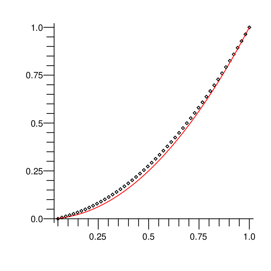
where N∈ℕN\in\mathbb{N} depends on the number of given boundary conditions. Since in the considered system x⁡(0)=0x(0)=0 and x⁡(1)=1x(1)=1, we take N=1N=1. Therefore, we get

z˙(t)=[∑k=01(αk)(t−a)k−αΓ⁡(k+1−α)x(k)(t))−2Γ⁡(2.5)t1.5]2.\dot{z}(t)=\left[\sum_{k=0}^{1}\binom{\alpha}{k}\frac{(t-a)^{k-\alpha}}{\Gamma(k+1-\alpha)}x^{(k)}(t))-\frac{2}{\Gamma(2.5)}t^{1.5}\right]^{2}.

Applying the classical Euler–Lagrange equation we obtain a second order differential equation, whose solution in shown on Figure 1.
Refer to caption
Figure 1: Numerical solution (dot line) vs exact solution (continuous line) in Example 3.

3.1 Higher-order fractional derivatives

In this subsection, we generalize the fractional Herglotz problem by considering higher-order fractional derivatives.

Theorem 4.

Consider the system

{z˙(t)=L(t,x(t),CaDαtx(t),z(t)), with t∈[a,b],z⁡(a)=za,xi(j)(a)=xi​aj,xi(j)(b)=xi​bj,\left\{\begin{array}[]{l}\dot{z}(t)=L(t,x(t),{{}^{C}_{a}D^{\alpha}_{t}}x(t),z(t)),\quad\mbox{ with }\,t\in[a,b],\\ z(a)=z_{a},\\ x_{i}^{(j)}(a)=x_{ia}^{j},\,x_{i}^{(j)}(b)=x_{ib}^{j},\end{array}\right. (10)

with for all i∈{1,…,n}i\in\{1,\ldots,n\} and j∈{0,…,i−1}j\in\{0,\ldots,i-1\}, where we assume that the following conditions:

  1. 1.

    αi∈(i−1,i)\alpha_{i}\in(i-1,i),

  2. 2.

    xi∈Cn​([a,b],ℝ)x_{i}\in C^{n}([a,b],\mathbb{R}), DtαaC​xi∈C1​([a,b],ℝ){{}^{C}_{a}D^{\alpha}_{t}}x_{i}\in C^{1}([a,b],\mathbb{R}),

  3. 3.

    za,xi​aj,xi​bjz_{a},x_{ia}^{j},x_{ib}^{j} are fixed reals,

  4. 4.

    the Lagrangian L:[a,b]×ℝ2​n+1→ℝL:[a,b]\times\mathbb{R}^{2n+1}\to\mathbb{R} is of class C1C^{1} and the maps t↦λ⁡(t)​∂L∂DtαiaC​xi​[x,z]​(t)t\mapsto\displaystyle\lambda(t)\frac{\partial L}{\partial{{}^{C}_{a}D^{\alpha_{i}}_{t}}x_{i}}[x,z](t), i∈{1,…,n}i\in\{1,\ldots,n\}, are such that Dbαit​(λ⁡(t)​∂L∂DtαiaC​xi​[x,z]​(t))\displaystyle{{}_{t}D^{\alpha_{i}}_{b}\left(\lambda(t)\frac{\partial L}{\partial{{}^{C}_{a}D^{\alpha_{i}}_{t}}x_{i}}[x,z](t)\right)} exist and are continuous on [a,b][a,b], where

    [x,z]​(t):=(t,x⁡(t),DtαaC​x​(t),z⁡(t))[x,z](t):=(t,x(t),{{}^{C}_{a}D^{\alpha}_{t}}x(t),z(t))
    andλ(t)=exp(−∫at∂L∂z[x,z](τ)dτ).\mbox{and}\quad\lambda(t)=\exp\left(-\int_{a}^{t}\frac{\partial L}{\partial z}[x,z](\tau)d\tau\right).

hold. If x=(x1,…,xn)x=(x_{1},\ldots,x_{n}) is such that z⁡[x;b]z[x;b] defined by (10) attains an extremum, then (x1,…,xn,z)(x_{1},\ldots,x_{n},z) satisfies the system of equations

λ(t)∂L∂xi[x,z](t)+Dbαit(λ(t)∂L∂DtαiaC​xi[x,z](t))=0,i=1,…,n,\lambda(t)\frac{\partial L}{\partial x_{i}}[x,z](t)+{{}_{t}D^{\alpha_{i}}_{b}\left(\lambda(t)\frac{\partial L}{\partial{{}^{C}_{a}D^{\alpha_{i}}_{t}}x_{i}}[x,z](t)\right)}=0,\quad i=1,\ldots,n, (11)

on [a,b][a,b].

Proof.

Let xx be such that z⁡[x;b]z[x;b] defined by (10) attains an extremum. Consider variations of type x+ϵ​ηx+\epsilon\eta with η=(η1,…,ηn)\eta=(\eta_{1},\ldots,\eta_{n}) satisfying ηi(j)​(a)=ηi(j)​(b)=0\eta_{i}^{(j)}(a)=\eta_{i}^{(j)}(b)=0, for all i∈{1,…,n}i\in\{1,\ldots,n\} and j∈{0,…,i−1}j\in\{0,\ldots,i-1\}. The rate of change of zz in the direction of η\eta is given by

θ⁡(t)=dd​ϵ​z​[x+ϵ​η;t]|ϵ=0​dd​ϵ=z⁡(t,x⁡(t)+ϵ​η​(t),DtαaC​x​(t)+ϵ​DtαaC​η​(t))|ϵ=0.\theta(t)=\frac{d}{d\epsilon}\left.z[x+\epsilon\eta;t]\right|_{\epsilon=0}\frac{d}{d\epsilon}=\left.z\left(t,x(t)+\epsilon\eta(t),{{}^{C}_{a}D^{\alpha}_{t}}x(t)+\epsilon{{}^{C}_{a}D^{\alpha}_{t}}\eta(t)\right)\right|_{\epsilon=0}.

Applying ϵ​η\epsilon\eta to differential equation in (10) we get

dd​t​z​[x+ϵ​η;t]=L⁡(t,x⁡(t)+ϵ​η​(t),DtαaC​x​(t)+ϵ​DtαaC​η​(t),z⁡[x+ϵ​η;t]).\frac{d}{dt}z[x+\epsilon\eta;t]=L(t,x(t)+\epsilon\eta(t),{{}^{C}_{a}D^{\alpha}_{t}}x(t)+\epsilon{{}^{C}_{a}D^{\alpha}_{t}}\eta(t),z[x+\epsilon\eta;t]).

Then, as in the proof of Theorem 3, we obtain the linear ODE with respect to θ\theta:

θ˙​(t)=∑i=1n[∂L∂xi​[x,z]​(t)​ηi​(t)+∂L∂DtαiaC​xi​[x]​(t)​DtαiaC​ηi​(t)]+∂L∂z​[x,z]​(t)​θ​(t).\dot{\theta}(t)=\sum_{i=1}^{n}\left[\frac{\partial L}{\partial x_{i}}[x,z](t)\eta_{i}(t)+\frac{\partial L}{\partial{{}^{C}_{a}D^{\alpha_{i}}_{t}}x_{i}}[x](t){{}^{C}_{a}D^{\alpha_{i}}_{t}}\eta_{i}(t)\right]+\frac{\partial L}{\partial z}[x,z](t)\theta(t).

Solving the linear ODE and using the fact that θ⁡(a)=θ⁡(b)=0\theta(a)=\theta(b)=0 we get

∫abλ⁡(t)​∑i=1n[∂L∂xi​[x,z]​(t)​ηi​(t)+∂L∂DtαiaC​xi​[x,z]​(t)​DtαiaC​ηi​(t)]​𝑑t=0.\int_{a}^{b}\lambda(t)\sum_{i=1}^{n}\left[\frac{\partial L}{\partial x_{i}}[x,z](t)\eta_{i}(t)+\frac{\partial L}{\partial{{}^{C}_{a}D^{\alpha_{i}}_{t}}x_{i}}[x,z](t){{}^{C}_{a}D^{\alpha_{i}}_{t}}\eta_{i}(t)\right]dt=0.

Integrating by parts we obtain

∫ab∑i=1n[λ⁡(t)​∂L∂xi​[x,z]​(t)+Dbαit​(λ⁡(t)​∂L∂DtαiaC​xi​[x,z]​(t))]​ηi​(t)​𝑑t\int_{a}^{b}\sum_{i=1}^{n}\left[\lambda(t)\frac{\partial L}{\partial x_{i}}[x,z](t)+{{}_{t}D^{\alpha_{i}}_{b}}\left(\lambda(t)\frac{\partial L}{\partial{{}^{C}_{a}D^{\alpha_{i}}_{t}}x_{i}}[x,z](t)\right)\right]\eta_{i}(t)dt
+[∑i=1n∑j=0i−1(−1)i−1−j​ηi(i−1−j)​(t)​Dbαi+j−it​(λ⁡(t)​∂L∂DtαiaC​xi​[x,z]​(t))]ab=0.+\left[\sum_{i=1}^{n}\sum_{j=0}^{i-1}(-1)^{i-1-j}\eta_{i}^{(i-1-j)}(t){{}_{t}D^{\alpha_{i}+j-i}_{b}}\left(\lambda(t)\frac{\partial L}{\partial{{}^{C}_{a}D^{\alpha_{i}}_{t}}x_{i}}[x,z](t)\right)\right]_{a}^{b}=0.

Since ηi(j)​(a)=ηi(j)​(b)=0\eta_{i}^{(j)}(a)=\eta_{i}^{(j)}(b)=0 for all i∈{1,…,n}i\in\{1,\ldots,n\} and j∈{0,…,i−1}j\in\{0,\ldots,i-1\}, and η\eta is arbitrary elsewhere, the theorem is proven. ∎

Next theorem generalizes transversality conditions given in Theorem 3.

Theorem 5.

Consider system (10) with an exception that xi(j)​(b)x_{i}^{(j)}(b) may take any value, for all i∈{1,…,n}i\in\{1,\ldots,n\} and j∈{0,…,i−1}j\in\{0,\ldots,i-1\}. If x=(x1,…,xn)x=(x_{1},\ldots,x_{n}) is such that z⁡[x;b]z[x;b] attains an extremum, then (x1,…,xn,z)(x_{1},\ldots,x_{n},z) satisfies the system of equations (11) on [a,b][a,b], and the transversality conditions

Dbαi+j−it​(λ⁡(t)​∂L∂DtαiaC​xi​[x,z]​(t))=0att=b,{{}_{t}D^{\alpha_{i}+j-i}_{b}}\left(\lambda(t)\frac{\partial L}{\partial{{}^{C}_{a}D^{\alpha_{i}}_{t}}x_{i}}[x,z](t)\right)=0\quad\mbox{at}\quad t=b,

for all i∈{1,…,n}i\in\{1,\ldots,n\} and all j∈{0,…,i−1}j\in\{0,\ldots,i-1\}.

3.2 Several independent variables

The fractional variational principle of Herglotz can be generalized to one involving several independent variables. In the following, the independent variables will be the time variable t∈[a,b]t\in[a,b] and the spacial coordinates x=(x1,…,xn)∈Ω=∏i=1n[ai,bi]x=(x_{1},\ldots,x_{n})\in\Omega=\prod_{i=1}^{n}[a_{i},b_{i}], n∈ℕn\in\mathbb{N}. The argument function of the functional z⁡[u;b]z[u;b] defined by the variational principle will be u=(u1​(t,x),…,um​(t,x))u=(u_{1}(t,x),\ldots,u_{m}(t,x)), m∈ℕm\in\mathbb{N}. In what follows, for α=(α1,…,αm)\alpha=(\alpha_{1},\ldots,\alpha_{m}) and βi=(βi,1,…,βi,m)\beta_{i}=(\beta_{i,1},\ldots,\beta_{i,m}), i=1,…,ni=1,\ldots,n we will use the following notation:

DtαaC​u=(Dtα1aC​u1,…,DtαmaC​um),{{}^{C}_{a}D^{\alpha}_{t}}u=({{}^{C}_{a}D^{\alpha_{1}}_{t}}u_{1},\ldots,{{}^{C}_{a}D^{\alpha_{m}}_{t}}u_{m}),
DxiβiaiCu=(Dxiβi,1aiCu1,…,Dxiβi,maiCum),i=1,…,n.{{}^{C}_{a_{i}}D^{\beta_{i}}_{x_{i}}}u=({{}^{C}_{a_{i}}D^{\beta_{i,1}}_{x_{i}}}u_{1},\ldots,{{}^{C}_{a_{i}}D^{\beta_{i,m}}_{x_{i}}}u_{m}),\quad i=1,\ldots,n.

The fractional variational principle with several independent variables is as follows:
Let the functional z=z⁡[u;b]z=z[u;b] of u=u⁡(t,x)u=u(t,x) be given by an integro-differential equation of the form

d​zd​t=∫ΩL⁡(t,x,u⁡(t,x),DtαaC​u​(t,x),Dx1β1a1C​u​(t,x),…,DxnβnanC​u​(t,x),z⁡(t))​dn​x,\frac{dz}{dt}=\displaystyle\int_{\Omega}L(t,x,u(t,x),{{}^{C}_{a}D^{\alpha}_{t}}u(t,x),{{}^{C}_{a_{1}}D^{\beta_{1}}_{x_{1}}}u(t,x),\ldots,{{}^{C}_{a_{n}}D^{\beta_{n}}_{x_{n}}}u(t,x),z(t))\,d^{n}x, (12)

t∈[a,b]t\in[a,b], where dn​x=d​x1​…​d​xnd^{n}x=dx_{1}\ldots dx_{n}; and let the following conditions be satisfied

  1. 1.

    u⁡(t,x)=g⁡(t,x)u(t,x)=g(t,x) for (t,x)∈∂P(t,x)\in\partial P, where P=[a,b]×ΩP=[a,b]\times\Omega, ∂P\partial P is the boundary of PP and g:∂P→Rmg:\partial P\rightarrow R^{m} is a given function;

  2. 2.

    αj,βi,j∈(0,1)\alpha_{j},\beta_{i,j}\in(0,1),

  3. 3.

    uj∈C1​(P,ℝ)u_{j}\in C^{1}(P,\mathbb{R}), DtαjaC​uj,Dxiβi,jaiC​uj∈C1​(P,ℝ){{}^{C}_{a}D^{\alpha_{j}}_{t}}u_{j},{{}^{C}_{a_{i}}D^{\beta_{i,j}}_{x_{i}}}u_{j}\in C^{1}(P,\mathbb{R}),

  4. 4.

    L:P×ℝm⁡(n+2)+1→ℝL:P\times\mathbb{R}^{m(n+2)+1}\to\mathbb{R} is of class C1C^{1} and the maps
    (t,x)↦λ⁡(t)​∂L∂DtαjaC​uj​[u,z]​(t,x)(t,x)\mapsto\displaystyle\lambda(t)\frac{\partial L}{\partial{{}^{C}_{a}D^{\alpha_{j}}_{t}}u_{j}}[u,z](t,x) and (t,x)↦λ⁡(t)​∂L∂Dxiβi,jaiC​uj​[u,z]​(t,x)(t,x)\mapsto\displaystyle\lambda(t)\frac{\partial L}{\partial{{}^{C}_{a_{i}}D^{\beta_{i,j}}_{x_{i}}}u_{j}}[u,z](t,x)
    are such that Dbαjt​(λ⁡(t)​∂L∂DtαjaC​uj​[u,z]​(t,x))\displaystyle{{}_{t}D^{\alpha_{j}}_{b}}\left(\lambda(t)\frac{\partial L}{\partial{{}^{C}_{a}D^{\alpha_{j}}_{t}}u_{j}}[u,z](t,x)\right) and Dbiβi,jxi​(λ⁡(t)​∂L∂Dxiβi,jaiC​uj​[u,z]​(t)){}_{x_{i}}D^{\beta_{i,j}}_{b_{i}}\left(\lambda(t)\frac{\partial L}{\partial{{}^{C}_{a_{i}}D^{\beta_{i,j}}_{x_{i}}}u_{j}}[u,z](t)\right) exist and are continuous on PP, where

    [u,z]​(t,x):=(t,x,u⁡(t,x),DtαaC​u​(t,x),Dx1β1a1C​u​(t,x),…,DxnβnanC​u​(t,x),z⁡(t)CLOSE,[u,z](t,x):=(t,x,u(t,x),{{}^{C}_{a}D^{\alpha}_{t}}u(t,x),{{}^{C}_{a_{1}}D^{\beta_{1}}_{x_{1}}}u(t,x),\ldots,{{}^{C}_{a_{n}}D^{\beta_{n}}_{x_{n}}}u(t,x),z(t),
    λ(t):=exp(−∫at∫Ω∂L∂z[u,z](τ,x)dnxdτ).\lambda(t):=\exp\left(-\int_{a}^{t}\int_{\Omega}\frac{\partial L}{\partial z}[u,z](\tau,x)d^{n}xd\tau\right).

for all i∈{1,…,n}i\in\{1,\ldots,n\} and j∈{0,…,m}j\in\{0,\ldots,m\}.

Consider η≡(η1​(t,x),…,ηm​(t,x))∈C1​([a,b]×Ω,ℝm)\eta\equiv(\eta_{1}(t,x),\ldots,\eta_{m}(t,x))\in C^{1}([a,b]\times\Omega,\mathbb{R}^{m}) that satisfies the boundary conditions η⁡(t,x)=0\eta(t,x)=0 for (t,x)∈∂P(t,x)\in\partial P and such that DtαjaC​ηj,Dxiβi,jaiC​ηj∈C1​(P,ℝ){{}^{C}_{a}D^{\alpha_{j}}_{t}}\eta_{j},{{}^{C}_{a_{i}}D^{\beta_{i,j}}_{x_{i}}}\eta_{j}\in C^{1}(P,\mathbb{R}). Then, the value of the functional z⁡[u;b]z[u;b] is an extremum for function uu which satisfy the condition

dd​ϵ​z​[u+ϵ​η;b]|ϵ=0=dd​ϵ​z​(b,[u]​(b,x))|ϵ=0=0,\frac{d}{d\epsilon}\left.z[u+\epsilon\eta;b]\right|_{\epsilon=0}=\frac{d}{d\epsilon}\left.z(b,[u](b,x))\right|_{\epsilon=0}=0, (13)

where [u]​(t,x):=(t,x,u⁡(t,x),DtαaC​u​(t,x),Dx1β1a1C​u​(t,x),…,DxnβnanC​u​(t,x)).[u](t,x):=(t,x,u(t,x),{{}^{C}_{a}D^{\alpha}_{t}}u(t,x),{{}^{C}_{a_{1}}D^{\beta_{1}}_{x_{1}}}u(t,x),\ldots,{{}^{C}_{a_{n}}D^{\beta_{n}}_{x_{n}}}u(t,x)). It should be pointed that when a variation ϵ​η\epsilon\eta is applied to uu the equation (12), defining the functional zz, must be solved with the same fixed initial condition zaz_{a} at t=at=a and the solution evaluated at the same fixed final time t=bt=b for all varied argument functions ϵ​η\epsilon\eta.

Theorem 6.

If uu is such that the functional z⁡[u;b]z[u;b] defined by equation (12) attains an extremum, then uu is a solution of the system of equations

λ⁡(t)​∂L∂uj​[u,z]​(t,x)+Dbαjt​(λ⁡(t)​∂L∂DtαjaC​uj​[u,z]​(t,x))+∑i=1nxiDβi,jbi(λ(t)∂L∂Dxiβi,jaiC​uj[u,z](t,x))=0,\lambda(t)\frac{\partial L}{\partial u_{j}}[u,z](t,x)+{{}_{t}D^{\alpha_{j}}_{b}}\left(\lambda(t)\frac{\partial L}{\partial{{}^{C}_{a}D^{\alpha_{j}}_{t}}u_{j}}[u,z](t,x)\right)\\ +\sum_{i=1}^{n}{{}_{x_{i}}D^{\beta_{i,j}}_{b_{i}}}\left(\lambda(t)\frac{\partial L}{\partial{{}^{C}_{a_{i}}D^{\beta_{i,j}}_{x_{i}}}u_{j}}[u,z](t,x)\right)=0, (14)

j=1,…,mj=1,\ldots,m.

Proof.

The idea of the proof is similar to that of the proof of Theorem 2. We show that equations (14) are a consequence of condition (13). The rate of change of zz, in the direction of η\eta, is given by

θ⁡(t)=dd​ϵ​z​[u+ϵ​η;t]|ϵ=0=dd​ϵ​z​(t,[u]​(t,x))|ϵ=0.\theta(t)=\frac{d}{d\epsilon}\left.z[u+\epsilon\eta;t]\right|_{\epsilon=0}=\frac{d}{d\epsilon}\left.z(t,[u](t,x))\right|_{\epsilon=0}. (15)

Applying the variation ϵ​η\epsilon\eta to the argument function in equation (12), differentiating with respect to ϵ\epsilon and then setting ϵ=0\epsilon=0 we get a differential equation for θ⁡(t)\theta(t):

d​θd​t(t)=∫Ω[∑j=1m∂L∂uj[u,z](t,x)ηj+∑j=1m∂L∂DtαjaC​uj[u,z](t,x)DtαjaCηj\frac{d\theta}{dt}(t)=\int_{\Omega}\left[\sum_{j=1}^{m}\frac{\partial L}{\partial u_{j}}[u,z](t,x)\eta_{j}+\sum_{j=1}^{m}\frac{\partial L}{\partial{{}^{C}_{a}D^{\alpha_{j}}_{t}}u_{j}}[u,z](t,x){{}^{C}_{a}D^{\alpha_{j}}_{t}}\eta_{j}\right.
+∑i=1n∑j=1m∂L∂Dxiβi,jaiC​uj[u,z](t,x)Dxiβi,jaiCηj+∂L∂z[u,z](t,x)θ(t)]dnx.\left.+\sum_{i=1}^{n}\sum_{j=1}^{m}\frac{\partial L}{\partial{{}^{C}_{a_{i}}D^{\beta_{i,j}}_{x_{i}}}u_{j}}[u,z](t,x){{}^{C}_{a_{i}}D^{\beta_{i,j}}_{x_{i}}}\eta_{j}+\frac{\partial L}{\partial z}[u,z](t,x)\theta(t)\right]d^{n}x.

Denoting

A(t)=∫Ω∑j=1m[∂L∂uj[u,z](t,x)ηj+∂L∂DtαjaC​uj[u,z](t,x)CaDαjtηj+∑i=1n∂L∂Dxiβi,jaiC​uj[u,z](t,x)CaiDβi,jxiηj]dnxA(t)=\int_{\Omega}\sum_{j=1}^{m}\left[\frac{\partial L}{\partial u_{j}}[u,z](t,x)\eta_{j}+\frac{\partial L}{\partial{{}^{C}_{a}D^{\alpha_{j}}_{t}}u_{j}}[u,z](t,x){{}^{C}_{a}D^{\alpha_{j}}_{t}}\eta_{j}\right.\\ \left.+\sum_{i=1}^{n}\frac{\partial L}{\partial{{}^{C}_{a_{i}}D^{\beta_{i,j}}_{x_{i}}}u_{j}}[u,z](t,x){{}^{C}_{a_{i}}D^{\beta_{i,j}}_{x_{i}}}\eta_{j}\right]d^{n}x

and

B⁡(t)=∫Ω∂L∂z​[u,z]​(t,x)​dn​x.B(t)=\int_{\Omega}\frac{\partial L}{\partial z}[u,z](t,x)d^{n}x.

we get

d​θd​t​(t)−B⁡(t)​θ​(t)=A⁡(t).\frac{d\theta}{dt}(t)-B(t)\theta(t)=A(t). (16)

Solving equation (16) and taking into consideration that θ⁡(a)=θ⁡(b)=0\theta(a)=\theta(b)=0 (see the proof of Theorem 2) we obtain

∫abλ⁡(t)​A​(t)​𝑑t=0.\int_{a}^{b}\lambda(t)A(t)dt=0.

Integrating by parts we get

∫ab∫Ω∑j=1m[λ(t)∂L∂uj[u,z](t,x)+Dbαjt(λ(t)∂L∂DtαjaC​uj[u,z](t,x))\int_{a}^{b}\int_{\Omega}\sum_{j=1}^{m}\left[\lambda(t)\frac{\partial L}{\partial u_{j}}[u,z](t,x)+{{}_{t}D^{\alpha_{j}}_{b}}\left(\lambda(t)\frac{\partial L}{\partial{{}^{C}_{a}D^{\alpha_{j}}_{t}}u_{j}}[u,z](t,x)\right)\right.
+∑i=1nDbiβi,jxi(λ(t)∂L∂Dxiβi,jaiC​uj[u,z](t,x))]ηjdnxdt=0\left.+\sum_{i=1}^{n}{{}_{x_{i}}D^{\beta_{i,j}}_{b_{i}}}\left(\lambda(t)\frac{\partial L}{\partial{{}^{C}_{a_{i}}D^{\beta_{i,j}}_{x_{i}}}u_{j}}[u,z](t,x)\right)\right]\eta_{j}d^{n}xdt=0

as η\eta satisfies the boundary conditions η⁡(a,x)=η⁡(b,x)=0\eta(a,x)=\eta(b,x)=0 for x∈Ωx\in\Omega, and η⁡(t,x)=0\eta(t,x)=0 for x∈∂Ωx\in\partial\Omega, a≤t≤ba\leq t\leq b. Finally, since ηj\eta_{j} are arbitrary functions, it follows that for all j∈{1,…,m}j\in\{1,\ldots,m\},

λ⁡(t)​∂L∂uj​[u,z]​(t,x)+Dbαjt​(λ⁡(t)​∂L∂DtαjaC​uj​[u,z]​(t,x))+∑i=1nDbiβi,jxi​(λ⁡(t)​∂L∂Dxiβi,jaiC​uj​[u,z]​(t,x))=0\lambda(t)\frac{\partial L}{\partial u_{j}}[u,z](t,x)+{{}_{t}D^{\alpha_{j}}_{b}}\left(\lambda(t)\frac{\partial L}{\partial{{}^{C}_{a}D^{\alpha_{j}}_{t}}u_{j}}[u,z](t,x)\right)+\\ \sum_{i=1}^{n}{{}_{x_{i}}D^{\beta_{i,j}}_{b_{i}}}\left(\lambda(t)\frac{\partial L}{\partial{{}^{C}_{a_{i}}D^{\beta_{i,j}}_{x_{i}}}u_{j}}[u,z](t,x)\right)=0 (17)

on [a,b]×Ω[a,b]\times\Omega. ∎

Remark 6.

We note that it is straightforward to obtain the transversality conditions for the Herglotz’s fractional variational problems with several variables (cf. [16]).

4 Noether-type theorem

Symmetric principles are key issues in mathematics and physics. There are close relationships between symmetries and conserved quantities. Noether first proposed the famous Noether symmetry theorem which describes the universal fact that invariance of the action functional with respect to some family of parameter transformations gives rise to the existence of certain conservation laws, i.e., expressions preserved along the solutions of the Euler-Lagrange equation. In this Section we extend Noether’s theorem to one that holds for fractional variational problems of Herglotz-type with one (Theorem 7) or several independent variables (Theorem 8).

Consider the one-parameter family of transformations

x¯j=hj(t,x,s),j=1,…,n,\bar{x}_{j}=h_{j}(t,x,s),\quad j=1,\ldots,n, (18)

depending on a parameter ss, s∈(−ε,ε)s\in(-\varepsilon,\varepsilon), where hjh_{j} are of class C2C^{2} and such that hj​(t,x,0)=xjh_{j}(t,x,0)=x_{j} for all j∈{1,…,n}j\in\{1,\ldots,n\} and for all (t,x)∈[a,b]×ℝn(t,x)\in[a,b]\times\mathbb{R}^{n}. By Taylor’s formula we have

hj​(t,x,s)=hj​(t,x,0)+s​ξj​(t,x)+o⁡(s)=xj+s​ξj​(t,x)+o⁡(s),h_{j}(t,x,s)=h_{j}(t,x,0)+s\xi_{j}(t,x)+o(s)=x_{j}+s\xi_{j}(t,x)+o(s), (19)

provided that |s|≤ε|s|\leq\varepsilon, where ξj​(t,x)=∂∂s​hj​(t,x,s)|s=0\xi_{j}(t,x)=\frac{\partial}{\partial s}h_{j}(t,x,s)|_{s=0}. For |s|≤ε|s|\leq\varepsilon the linear approximation to transformation (18) is x¯j≈xj+s​ξj​(t,x)\bar{x}_{j}\approx x_{j}+s\xi_{j}(t,x).
This transformation leads, for any fixed sufficiently small parameter ss and any fixed function x⁡(⋅)=(x1​(⋅),…,xn​(⋅))x(\cdot)=(x_{1}(\cdot),\ldots,x_{n}(\cdot)), to x¯​(⋅)=(x¯1​(⋅),…,x¯n​(⋅))\overline{x}(\cdot)=(\overline{x}_{1}(\cdot),\ldots,\overline{x}_{n}(\cdot)) given by

x¯j(t)=hj(t,x(t),s),j=1,…,n.\bar{x}_{j}(t)=h_{j}(t,x(t),s),\quad j=1,\ldots,n.

Denote by θ=θ⁡(t)\theta=\theta(t) the total variation produced by the family of transformations (19), that is

θ⁡(t)=dd​s​z¯​[x+s​ξ;t]|s=0.\theta(t)=\frac{d}{ds}\left.\bar{z}[x+s\xi;t]\right|_{s=0}. (20)

We define the invariance of the functional zz, defined by differential equation (1), under transformation (19) as follows.

Definition 1.

The transformation (19) leaves the functional zz, defined by differential equation (1), invariant if θ⁡(t)≡0\theta(t)\equiv 0.

Remark 7.

When s=0s=0, the following holds z¯​[x¯;t]=z​[x;t]\bar{z}[\bar{x};t]=z[x;t].

Theorem 7.

If the functional zz defined by differential equation (1) is invariant in the sense of definition 1, then

∑j=1n𝒟αj​[λ⁡(t)​∂L∂DtαjaC​xj​[x,z]​(t),ξj​(t,x)]=0,\sum_{j=1}^{n}\mathcal{D}^{\alpha_{j}}\left[\lambda(t)\frac{\partial L}{\partial{{}^{C}_{a}D^{\alpha_{j}}_{t}}x_{j}}[x,z](t),\xi_{j}(t,x)\right]=0, (21)

where λ(t):=exp(−∫at∂L∂z[x,z](τ)dτ)\lambda(t):=\exp\left(-\int_{a}^{t}\frac{\partial L}{\partial z}[x,z](\tau)d\tau\right) and 𝒟α​[f,g]:=f​DtαaC⋅g−g⋅Dbαt​f\mathcal{D}^{\alpha}[f,g]:=f{{}^{C}_{a}D^{\alpha}_{t}}\cdot g-g\cdot{{}_{t}D^{\alpha}_{b}}f, holds along the solutions of the generalized fractional Euler–Lagrange equations (3).

Proof.

Applying transformations (19) to equation (1) we get

dd​t​z¯=L⁡(t,x¯​(t),DtαaC​x¯​(t),z¯​(t)).\frac{d}{dt}\bar{z}=L(t,\bar{x}(t),{{}^{C}_{a}D^{\alpha}_{t}}\bar{x}(t),\bar{z}(t)). (22)

Differentiating both sides of (22) with respect to ss and then setting s=0s=0, we get a differential equation for θ⁡(t)\theta(t)

θ˙​(t)−∂L∂z​[x,z]​(t)​θ​(t)=∑j=1n(∂L∂xj​[x,z]​(t)​ξj​(t)+∂L∂DtαjaC​xj​[x,z]​(t)​DtαjaC​ξj​(t))\dot{\theta}(t)-\frac{\partial L}{\partial z}[x,z](t)\theta(t)=\sum_{j=1}^{n}\left(\frac{\partial L}{\partial x_{j}}[x,z](t)\xi_{j}(t)+\frac{\partial L}{\partial{{}^{C}_{a}D^{\alpha_{j}}_{t}}x_{j}}[x,z](t){{}^{C}_{a}D^{\alpha_{j}}_{t}}\xi_{j}(t)\right)

whose solution is

θ⁡(t)​λ​(t)−θ⁡(a)=∫at∑j=1n(∂L∂xj​[x,z]​(τ)​ξj​(τ)+∂L∂DταjaC​xj​[x,z]​(τ)​DταjaC​ξj​(t))​λ​(τ)​𝑑τ\theta(t)\lambda(t)-\theta(a)=\int_{a}^{t}\sum_{j=1}^{n}\left(\frac{\partial L}{\partial x_{j}}[x,z](\tau)\xi_{j}(\tau)+\frac{\partial L}{\partial{{}^{C}_{a}D^{\alpha_{j}}_{\tau}}x_{j}}[x,z](\tau){{}^{C}_{a}D^{\alpha_{j}}_{\tau}}\xi_{j}(t)\right)\lambda(\tau)d\tau

with notation λ(t)=exp(−∫at∂L∂z[x,z](τ)dτ)\lambda(t)=\exp\left(-\int_{a}^{t}\frac{\partial L}{\partial z}[x,z](\tau)d\tau\right). Observe that θ⁡(a)=0\theta(a)=0, also by hypothesis θ⁡(τ)=0\theta(\tau)=0 for arbitrary τ\tau. Thus

0=∫aτ∑j=1n(∂L∂xj​[x,z]​(t)​ξj​(t)+∂L∂DtαjaC​xj​[x,z]​(t)​DtαjaC​ξj​(t))​λ​(t)​𝑑t0=\int_{a}^{\tau}\sum_{j=1}^{n}\left(\frac{\partial L}{\partial x_{j}}[x,z](t)\xi_{j}(t)+\frac{\partial L}{\partial{{}^{C}_{a}D^{\alpha_{j}}_{t}}x_{j}}[x,z](t){{}^{C}_{a}D^{\alpha_{j}}_{t}}\xi_{j}(t)\right)\lambda(t)dt

On the solutions of the generalized fractional Euler–Lagrange equations (3) we have

0=∑j=0n[λ(t)∂L∂aCDtαj​xj​[x,z]​(t)DtαjaCξj(t,x)−tDbαj(λ(t)∂L∂aCDtαj​xj​[x,z]​(t))ξj(t,x)].0=\sum_{j=0}^{n}\left[\lambda(t)\frac{\partial L}{\partial^{C}_{a}D^{\alpha_{j}}_{t}x_{j}[x,z](t)}{{}^{C}_{a}D^{\alpha_{j}}_{t}}\xi_{j}(t,x)-_{t}D^{\alpha_{j}}_{b}\left(\lambda(t)\frac{\partial L}{\partial^{C}_{a}D^{\alpha_{j}}_{t}x_{j}[x,z](t)}\right)\xi_{j}(t,x)\right].

By definition of operator 𝒟α\mathcal{D}^{\alpha} we obtain equation (21). ∎

Example 4.

Consider the Lagrangian in one spatial dimension

L(t,x(t),DtαaCx(t),z(t))=f(aCDtαx)−γz,L(t,x(t),{{}^{C}_{a}D^{\alpha}_{t}}x(t),z(t))=f(^{C}_{a}D^{\alpha}_{t}x)-\gamma z, (23)

where ff is a C1C^{1} function and γ\gamma is a positive constant. Obviously, the Lagrangian (23) is invariant under transformation

x¯​(t)=x​(t)+c,\bar{x}(t)=x(t)+c,

where cc is a constant. Therefore, Theorem 7 indicates that

𝒟α[eγ​tf′(aCDtαx),c]=0,\mathcal{D}^{\alpha}\left[e^{\gamma t}f^{\prime}(^{C}_{a}D^{\alpha}_{t}x),c\right]=0, (24)

along any solution of Dbαt(eγ​tf′(aCDtαx))=0{}_{t}D^{\alpha}_{b}\left(e^{\gamma t}f^{\prime}(^{C}_{a}D^{\alpha}_{t}x)\right)=0. Notice that equation (24) can be written in the form dd​t(Ib1−αt(eγ​tf′(aCDtαx)))=0\frac{d}{dt}\left({}_{t}I^{1-\alpha}_{b}\left(e^{\gamma t}f^{\prime}(^{C}_{a}D^{\alpha}_{t}x)\right)\right)=0, that is, the quantity

Ib1−αt(eγ​tf′(aCDtαx)){}_{t}I^{1-\alpha}_{b}\left(e^{\gamma t}f^{\prime}(^{C}_{a}D^{\alpha}_{t}x)\right)

following the classical approach, can be called a generalized fractional constant of motion.

Now we generalize Theorem 7 to the case of several independent variables. For that consider the one-parameter family of transformations

u¯j=hj(t,x,u,s),j=1,…,m\bar{u}_{j}=h_{j}(t,x,u,s),\quad j=1,\ldots,m (25)

depending on a parameter ss, s∈(−ε,ε)s\in(-\varepsilon,\varepsilon), where hjh_{j} are of class C2C^{2} and such that hj​(t,x,u,0)=uj​(t,x)h_{j}(t,x,u,0)=u_{j}(t,x) for all j∈{1,…,m}j\in\{1,\ldots,m\} and for all (t,x,u)∈[a,b]×Ω×ℝm(t,x,u)\in[a,b]\times\Omega\times\mathbb{R}^{m}. As before for |s|≤ε|s|\leq\varepsilon the linear approximation to transformation (25) is u¯j≈uj+s​ξj​(t,x,u)\bar{u}_{j}\approx u_{j}+s\xi_{j}(t,x,u), where ξj​(t,x,u)=∂∂s​hj​(t,x,u,s)|s=0\xi_{j}(t,x,u)=\frac{\partial}{\partial s}h_{j}(t,x,u,s)|_{s=0}. The following result generalizes Theorem 7, and can be proved in a similar way (cf. [17])

Theorem 8.

Let the functional zz, defined by differential equation (12), is invariant under the family of transformations (25). Then

∑j=1n{𝒟αj[λ(t)∂L∂DtαjaC​uj[u,z](t,x),ξj(t,x,u)]+∑i=1n𝒟βj,i[λ(t)∂L∂Dxiβi,jaiC​uj[u,z](t,x),ξj(t,x,u)]}=0,\sum_{j=1}^{n}\left\{\mathcal{D}^{\alpha_{j}}\left[\lambda(t)\frac{\partial L}{\partial{{}^{C}_{a}D^{\alpha_{j}}_{t}}u_{j}}[u,z](t,x),\xi_{j}(t,x,u)\right]\right.\\ \left.+\sum_{i=1}^{n}\mathcal{D}^{\beta_{j,i}}\left[\lambda(t)\frac{\partial L}{\partial{{}^{C}_{a_{i}}D^{\beta_{i,j}}_{x_{i}}}u_{j}}[u,z](t,x),\xi_{j}(t,x,u)\right]\right\}=0,

where λ(t):=exp(−∫at∫Ω∂L∂z[u,z](τ,x)dnxdτ)\lambda(t):=\exp\left(-\int_{a}^{t}\int_{\Omega}\frac{\partial L}{\partial z}[u,z](\tau,x)d^{n}xd\tau\right) and 𝒟α​[f,g]:=f​DtαaC⋅g−g⋅Dbαt​f\mathcal{D}^{\alpha}[f,g]:=f{{}^{C}_{a}D^{\alpha}_{t}}\cdot g-g\cdot{{}_{t}D^{\alpha}_{b}}f, holds along the solutions of the generalized fractional Euler–Lagrange equations (14).

Acknowledgements

Ricardo Almeida is supported by Portuguese funds through the CIDMA - Center for Research and Development in Mathematics and Applications, and the Portuguese Foundation for Science and Technology (“FCT–Fundação para a Ciência e a Tecnologia”), within project PEst-OE/MAT/UI4106/2014. Agnieszka B. Malinowska is supported by the Bialystok University of Technology grant S/WI/02/2011. We thank the anonymous reviewer for his careful reading of our manuscript and his many insightful comments and suggestions.

References

  • [1] D. V. Anosov, S. K. Aranson, V. I. Arnold, I. U. Bronshtein, V. Z. Grines and Y.S. Ilyashenko, “Ordinary Differential Equations and Smooth Dynamical Systems”, Encyclopaedia of Mathematical Sciences, Vol. 1, 1988.
  • [2] T. M. Atanacković, S. Konjik and S. Pilipović, Variational problems with fractional derivatives: Euler-Lagrange equations, J Phys A 41 (2008), no. 9, 095201, 12 pp.
  • [3] T. M. Atanacković and B. Stanković, On a numerical scheme for solving differential equations of fractional order, Mech. Res. Comm. 35 (2008), no. 7, 429–438.
  • [4] G. S. F. Frederico and D. F. M. Torres, A formulation of Noethers theorem for fractional problems of the calculus of variations, J. Math. Anal. Appl. 334 (2007), no. 2, 834–846.
  • [5] N. J. Ford and M. L. Morgado, Fractional boundary value problems: Analysis and Numerical methods, Fract. Calc. Appl. Anal. 14 (2011), no. 4, 554–567.
  • [6] N.J. Ford and M.L. Morgado, Distributed order equations as boundary value problems, Comput. Math. Appl. 64 (2012), no. 10, 2973–2981.
  • [7] B. Georgieva and R. Guenther, First Noether-type theorem for the generalized variational principle of Herglotz, Topol. Methods Nonlinear Anal. 20 (2002), no. 2, 261–273.
  • [8] B. Georgieva and R. Guenther, Second Noether-type theorem for the generalized variational principle of Herglotz, Topol. Methods Nonlinear Anal. 26 (2005), no. 2, 307–314.
  • [9] B. Georgieva, R. Guenther and T. Bodurov, Generalized variational principle of Herglotz for several independent variables. First Noether-type theorem, J. Math. Phys. 44 (2003), no. 9, 3911–3927.
  • [10] H. Goldstein, “Classical Mechanics”, Addison-Wesley Press, Inc., Cambridge, MA, 1951.
  • [11] R. B. Guenther, C. M. Guenther and J. A. Gottsch, “The Herglotz Lectures on Contact Trans- formations and Hamiltonian Systems”, Lecture Notes in Nonlinear Analysis, Vol. 1, Juliusz Schauder Center for Nonlinear Studies, Nicholas Copernicus University, Toruń, 1996.
  • [12] G. Herglotz, Berührungstransformationen, “Lectures at the University of Göttingen”, Göttingen, 1930.
  • [13] A. A. Kilbas, H. M. Srivastava, J. J. Trujillo, “Theory and applications of fractional differential equations”, North-Holland Mathematics Studies, 204. Elsevier Science B.V., Amsterdam, 2006.
  • [14] M. Klimek, “On solutions of linear fractional differential equations of a variational type”, The Publishing Office of Czenstochowa University of Technology, Czestochowa, 2009.
  • [15] C. Lánczos, “The variational principles of mechanics”, fourth edition, Mathematical Expositions, No. 4, Univ. Toronto Press, Toronto, ON, 1970.
  • [16] A. B. Malinowska and D. F. M. Torres, “Introduction to the fractional calculus of variations”, Imp. Coll. Press, London, 2012.
  • [17] A. B. Malinowska, A formulation of the fractional Noether-type theorem for multidimensional Lagrangians, Appl. Math. Lett. 25 (2012) no. 11, 1941-1946.
  • [18] V. J. Menon, N. Chanana and Y. Singh, A Fresh Look at the BCK Frictional Lagrangian, Prog. Theor. Phys. 98 (1997), no. 2, 321–329.
  • [19] I. Podlubny, “Fractional differential equations, Mathematics in Science and Engineering”, 198. Academic Press, Inc., San Diego, CA, 1999.
  • [20] S. Pooseh, R. Almeida and D. F. M. Torres, Approximation of fractional integrals by means of derivatives, Comput. Math. Appl. 64 (2012), no. 10, 3090–3100.
  • [21] F. Riewe, Nonconservative Lagrangian and Hamiltonian mechanics, Phys. Rev. E (3)53 (1996), no. 2, 1890–-1899.
  • [22] S. G. Samko, A. A. Kilbas and O. I. Marichev, “Fractional integrals and derivatives”, translated from the 1987 Russian original, Gordon and Breach, Yverdon, 1993.
  • [23] S. Santos, N. Martins, D. F. M. Torres, Higher-order variational problems of Herglotz type, will appear in Vietnam Journal of Mathematics.

Received ; revised .