Scaling Properties of Urban Facilities
Abstract
Two measurements are employed to quantitatively investigate the scaling properties of the spatial distribution of urban facilities, the function by number counting and the variance-mean relationship with the method of expanding bins. The function and the variance-mean relationship are both power functions. It means that the spatial distribution of urban facilities are scaling invariant. Further analysis of more data (which includes 8 types of facilities in 37 major Chinese cities) shows that the exponents of the power function do not have systematic variations across facilities and cities, which suggests the possibility that the scaling rule is universal. A double stochastic process (DSP) model is proposed such that the two empirical results can both be embedded. Simulation of DSP yields better agreement with the urban data than of the correlated percolation model.
I Introduction
There has been an increasing interest to study cities and urban lives mainly due to our increasing ability to collect data which gives us better clues how cities are functioning. Some empirical regularities have been established about cities. Most urban properties, such as, land area, socio-economic rate, etc, vary continuously with population size and are well described mathematically as power-law scaling relations[1, 2]. The size distribution of cities also fits a power function (known as Zipf’s law): the number of cities with populations greater than is proportional to [3]. Geometrically, the complex spatial structure of cities have apparent fractal nature associated with individual cities and entire urban systems[4].
Most traditional research of city geography focus on cities or city clusters. Providers of electronic maps such as Google and Baidu give us access to spatial structure data at the sub-scales of cities. These data records spatial coordinate information of numerous urban facilities. China has been experiencing the largest urbanization process in human history. About 300 million people move to cities in the last 2 decades[16]. As a response, many urban facilities have been developed to satisfy their needs. It is of special interest how these facilities are spatially organized during their rapid development.
In this paper, we present evidence that spatial distribution of urban facilities, much alike that of city clusters, are statistically self-similar at all scales. Two measurements are employed to confirm these findings. The first measurement is the second-order statistics function by number counting[7]. Derivative of function gives the pair correlation and covariance functions. If the deviation of from its complete spatial randomness(CSR) version is a power function , it means that the pair correlation is also a power function. The second measurement is the method of expanding bins. The variance and average number of events in a series of expanding bins are related by a power function , which also implies a self-similar scaling property of urban facilities[8]. The two methods are closely related to each other. The exponents and are found to satisfy in our empirical results. However, they are not completely redundant. Some model, e.g., the correlated percolation model (CPM) does not produce the desired variance-mean relationship even though the fitted spatial covariance function is imposed to its random field.
One goal of this paper is to understand whether the power law of variance-mean and power law autocorrelation function indicate a universal scaling rule about urban facilities. By doing so, we apply the two methods to a lot of spatial data of urban facilities, which includes 8 facilities in 37 major Chinese cities. The power laws seem to hold for all combinations of facilities and cities, so does the relationship of the exponents . Then as the other goal of this paper, we propose a mathematical model of double stochastic process (DSP) in which the two empirical findings can both be embedded. The DSP model resembles the actual process of urban facilities in the sense that urban facilities are developing on top of the existing structure of a city while the city structure itself can also be modelled as a stochastic process. One possible explanation of the scaling ”universality” of urban facilities is that they come from the same source of the scaling invariance of the environment of the city, which could result from the fractal nature of geographic characteristics of the city[5] or the fractal residential settlement[6]. However this picture does not rule out the possibility that the scaling property of urban facilities is from some type of critical process arising from interactions between the facilities and city environment and among the facilities themselves. The double stochastic process is a mathematical framework which models the macro statistical properties of urban facilities and ignores the underlying interactions.
There are two ways to generate point patterns with scaling invariance. One way is to have a lattice model in which the point patterns are formed according to some rules on a lattice. Diffusion limited aggregation (DLA) is such a model in which particles are added on at a time and move randomly until they join the cluster[9, 10]. The model produces the desirable fractional power-law behaviour of the correlation function. One concern when applying DLA model to urban systems is that the treelike dendritic structures generated from DLA model does not resemble the actual spatial morphology[12]. Also urban systems do not have obvious central places as seen in DLA model.
Another method is to assume that underlying the discrete point pattern there is a continuous random field. The spatial correlation properties of the point patterns can be imposed to the random field. Correlated percolation model(CPM) puts the idea into practice to model city growth[12], which takes the development process of a city cluster as correlated rather than being added to the cluster at random. With slight different notations as in the paper, we summarize CPM as follows. The model generates a Gaussian random process with a long range power correlation function. By choosing a spatial varying occupancy probability , the model can control the spatial concentration of population density. For a realization of random field , the discretized occupancy sequence is determined by , where is the cumulative distribution function of the Gaussian random variable and is the Heaviside step function. The model is very successful in modelling both dynamics of city development and static statistical properties of the perimeter of the city cluster and power law distributions of urban settlements.
It is appealing to apply CPM to urban facilities as the subscale analogy to city clusters. However, as shown in Appendix, CPM does not produce if the covariance structure of function is imposed to the random field . The scaling property of variance-mean relationship rely on the covariance of after a threahold is set to generate point patterns. On the other hand, the two empirical scaling properties can be easily embedded in DSP model. Besides, CPM does not generate the same results when we generate the discrete point patterns and change the scale of discretization. The Heaviside function is either 0 or 1. For example, when threshold is chosen, if both and , then . If a larger discretization scale is taken to combine and to one vertex, , then . Thanks to the additivity of Poisson distribution, DSP gives the same results when applied to different scales of discretization. In this case, , . The additivity is preserved.
In this paper, DSP and CPM are both implemented for comparison. DSP fits the variance and mean power relationship closer to empirical results than CPM.
II Methods and Data
II.1 Pair Correlation and function
In the continuous limit of a point pattern, we can define a random field . As the tradition, an upper case letter is used to denote a random variable, and lower case one to denote a sample. In spatial point analysis[11], the first and second order properties of point pattern are described by its intensity function , and second-order intensity function . Covariance density function which measures the covariance of number of events at two infinitesimal regions and can be written as
| (1) |
where . For a stationary isotropic point process, is a constant, covariance density function only depends on distance between two spatial locations.
One way to estimate the covariance density is through the function by number counting, which is defined as,
| (2) |
where is the number of further events within distance of an arbitrary event. It can be shown that [11].
For a point process with complete spatial randomness (CSR), one has . If the deviation of from CSR version is a power function, e.g., , then,
| (3) |
II.2 Method of Expanding Bins
Another way to analyze scaling properties of point pattern is the method of expanding bins. A set of equal-sized non-overlapping bins are introduced to divide the urban area of a city into equal-sized segments, the size of each bin is , is the area of the whole city. The number of facilities is counted for each bin . We assume that the distribution of urban facilities are homogeneous, thus, the sample variance and the average number of facilities in an area of size can be estimated as, . If and are related by a power function as the size of bin to divide the city varies, it implies a statistically self-similar scaling of the spatial distribution[8]. This method does not assume a stochastic process for the point pattern. If the point pattern is generated from stochastic model, e.g., from a underlying Poisson process with spatial non-homogeneous density , the power law relationship of variance and average number of events implies that the Poisson density is a spatially correlated with a power covariance density , and the two exponents are related by as will be shown in appendix. Since can be given by Eq. 3, then and are related by .
II.3 Data Source
Through Baidu Map API, we record urban data of subscale structures which includes the spatial coordinates of 8 urban facilities in the city area and adjacent counties and county-level cities of 37 major Chinese cities. The 8 facilities are: beauty salons, banks, stadiums, schools, pharmacy, convenient stores, restaurants and tea houses. The 37 major cities consist of 4 direct-controlled municipalities (Beijing, Shanghai, Chongqing and Tianjin), 30 Provincial capitals and sub-provincial cities and 3 other large cities. The spatial data is the latitude and longitude coordinates of each facility. The spatial data of the latitude and longitude spherical coordinates is converted to the plane coordinate data denoted by meters (data is all rounded to meter). Since it is hard to define the exact boundary of a city, we fix a central point of the city, and only consider those events fallen into a square lattice centered around the central point. The bins size is chosen from meters to meters at interval of meters in the method of expanding bins. When calculating the function, is chosen from meters to meters at increasing interval so that in log-log plot the distance somehow spreads uniformly.
III Empirical Results
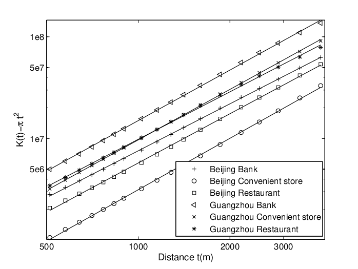

As an example to show the scaling properties, we choose 3 facilities (banks, convenient stores and restaurants) in Beijing and Guangzhou, the largest city in the northern and southern China. There are 6 combinations out of 3 facilities and 2 cities. As shown in Fig. 1(a), The straight lines of in a log-log plot indicates that is a power function. The exponents have very close values for 6 combinations. On the other hand, variance and average number of events are related by a power function as the bin size varies in the method of expanding bins. The exponents and are related by . The exact values of these exponents are listed in Table. 1.
| f | b | 1+f/2 | |
|---|---|---|---|
| Beijing Bank | 1.53 0.013 | 1.770.04 | 1.77 0.006 |
| Beijing Convenient Store | 1.68 | 1.820.04 | 1.84 0.009 |
| Beijing Restaurant | 1.61 | 1.810.03 | 1.800.010 |
| Guangzhou Bank | 1.65 0.020 | 1.850.04 | 1.82 0.010 |
| Guangzhou Convenient Store | 1.650.010 | 1.850.02 | 1.82 0.005 |
| Guangzhou Restaurant | 1.550.020 | 1.81 0.03 | 1.770.010 |
One goal of this paper is to understand whether the scaling invariance of urban facilities is universal. For this purpose, we apply the same analysis to all 8 facilities and 37 cities. The power function of both the function and the variance-mean relationship seem to hold for all combinations. The exponents of are reported in Fig. 2. In order to plot the results together, 8 cities are excluded for which there is not enough sample data to estimate variance-mean for at least one facility. We tend to believe that these exponents are universal in the sense that: (a) they do not have any systematic variations across 8 urban facilities regardless of their different nature of business or different concentrations in each city, (b) they do not show significant dependence on city regardless of the dramatic difference in population size, geographical characteristics, tradition of city planing from big cities such as Beijing to small cities such as Yinchuan. The error bars only indicate the statistical errors from linear regression. The variations of the exponents from the average value of all cities in Fig. 2 may be explained by other sources of errors. For example, the fixed choice of area for each city may violate the stationery assumption as in some region of a city, e.g. a harbour city, there are not facilities at all.


IV A Double Stochastic Process Model
The other purpose of this paper is to propose a mathematical model in which the two power law rules, i.e., the power law of the spatial covariance and that of variance-mean relationship, can be embedded. It should be noted that only the first and second statistics are reflected in the power law rules. More information is needed, e.g., higher order statistics, in order to construct more realistic models.
CPM has been successfully applied to model the growth of city clusters. It is reasonable to visualize city development as addition of new units to the perimeter of an existing system. Urban facilities, on the other hand, is developing on top of an existing city structure. Besides the stochastic nature of the urban growth, another stochastic process is needed to model the randomness of the locating of urban facilities. Another reason we propose DSP is that it can predit the relationship of the exponents of two power law functions .
The first layer stochastic process of DSP is a random field of density function , which models the inhomogeneous concentration of facilities in a city. The density function is a correlated random field to reflect the spatial heterogeneity of the city. Similar to correlated percolation model, the density function is long-range correlated, which takes account of the fractal structure of the city. Conditioned on the density, the locating of urban facilities is based on a Poisson process rather than a threshold cut off. This type of point process is called Cox process in the spatial point analysis. One reason to use Poisson process to generate the point patterns is due to the additivity of Poisson distribution. The summation of two independent Poisson distributed random variables is still Poisson distributed. This property is important for our model to explain the scaling invariant properties implied by the power law relationship between the variance and mean.


As in the appendix, we see that if the covariance of the random field is a power function , the resulted point pattern, which is generated from a Poisson process conditioned on the random field as its density, is scaling invariant. The power law relationship between the variance and average number can be inherited from the power function of the covariance. The exponents of two power functions are related by .
A relatively flexible and tractable construction to encompass the non-negative constraint for density processes is log-Gaussian processes[13]. The density function is drawn from a log-Gaussian random process . is assumed to be a stationery isotropic Gaussian, . Its spatial depedence is given by its covariance density . The first order and second order statistics of and fields are related by[11], , and . Once we know the covariance of the target field , we can calculate the covarince of the Gaussian random field field .
In summary, the spatial point pattern is generated in two steps: (1)a Gaussian random field is sampled with desired covariance structure. is thus obtained which is the density function of the point pattern; (2)a point pattern is generated for each vertex in the lattice independently. An interger is assigned to each vertex following a Poisson distribution .
V Simulations
We take banks in Beijing as an example. If the precision of the planar coordinate data is set to be 1 meter, the original data of the big Beijing area is on a lattice, too big for a PC to simulate. The data is mapped to a lattice by taking a transformation of the coordinate of each point as , rounded to its nearest integer. Its function is estimated as . Knowing the total number of sample points in the system, one can estimate as .
The sample point pattern is generated from two steps as described above. First, an isotropic and stationary Gaussian random field is generated with the covariance function given as,
| (4) |
Since , diverges at . We take an approximation for the correlation function which asymptotically has the same power-law behaviour. A Gaussian random field with a given covariance can be generated from the Fourier filtering method [14, 12].
In order to have a field with desired expected value . We set the expected value for Gaussian field as . The next step is to sample the point pattern. Number of events for each vertex is sampled independently as .
The results are reported in Fig. 3 and Fig. 4. In Fig. 3, we use data of banks in the big Beijing area. Fig. 3(a) is the spatial distribution of banks in the big Beijing area. Fig. 3(b) is a random sample from the log-normal double stochastic model by setting , which is estimated from the real data. In Fig. 3(c), we report the covariance of the real data compared with the simulation data averaged over 50 samples. The covariance of the simulation data as denoted by the solid line is estimated from the power spectral of by fast Fourier transform[15]. We see that the covariance function fits pretty well although is not directly sampled. Fig. 3(d), the relationship of the variance-mean is reported in a log-log plot for the real data in comparison with the simulation result averaged over 50 samples. As we can see from the Fig. 3(d), the variance for the real data denoted by dashed line is slightly bigger than that of the simulation data. This is due to the fact that the real data of banks is highly concentrated in the metropolitan area of Beijing. In Fig. 3(a), there are not too many banks in the outer perimeter of the big Beijing area. It thus creates bigger variance when averaged over the whole big Beijing area than the simulation data. While in simulation, we assume the density field is stationery. One can cope with this problem by choosing a spatial varying adjustment to the field. It is not the topic of this paper. Instead, we constrain the data to the metropolitan area of Beijing which covers and redo the simulation. As shown in Fig. 4(d), the fitting of the variance-mean is much better.
As comparison, we generate the point pattern from the correlated percolation model which is a single stochastic process. Now, is directly fed in as a covariance function to generate a Gaussian random field . The discrete point pattern is then generated by applying a threshold to the Gaussian field. We set if . The experiment is run on the metropolitan area of Beijing. The result is reported in Fig. 5. As we can see from Fig. 5(b), the resulted point pattern is highly aggregated and form isolated clusters. By setting the threshold as , we have the exact same number of points as the real data. The occupancy probability which equals to is far below the critical concentration threshold of a lattice percolation system. The resulted point pattern is composed of isolated clusters. We can see from Fig. 5(d), the variance of the simulation data, denoted by a solid line is much bigger than that of the real data. It does not fit as well as the double stochastic model.
VI Conclusion and discussion
In this paper, we use a lot of spatial data of urban facilities in Chines major cities, which are closely related to people’s everyday lives to investigate their scaling properties. One purpose of this paper is to understand whether the spatial distribution of urban facilities are scaling invariant and whether the scaling rule is universal. Two measurments are employed to quantitatively investigate the scaling properties of the spatial distribution of urban facilities, the function from the spatial analysis and variance-mean relationship from the method of expanding bins. The function and the variance-mean relationship are both power functions, which indicate that the spatial distribution of urban facilities are scaling invariant. Further analysis of 8 facilities in 37 major Chinese cities shows that the exponents of the power function do not have systematic variations with city or facility, which suggests the possibility that the scaling rule is universal. In addition, the exponent of the function and of the variance-mean are related by . The two measurements are not completely redundant. Some model, e.g. the correlated percolation model(CPM) does not produce the desired variance-mean relationship although the fitted spatial covariance function is imposed to its random field.
The other purpose of this paper is to propose a double stochastic process (DSP) model in which the two power law rules can be embedded. The DSP model assumes that there is a correlated random field underlying the spatial point pattern. CPM successfully puts the idea of random field to model city growth. However, the cut off by applying a threshold in CPM does not preserve the additivity of random field during the scale change, so that it can not be applied to different scales of discretization. The other reason is that CPM does not predict the desired relationship between the two exponents in the point patterns generated from the random field to which the covariance function implied from the empirical function is imposed. Comparison between the two models are made with simulations. The results from DSP model agree better with real urban data than those from CPM.
Although the assumption of the existence of a scaling invariant random field is for mathematical convenience, it resembles the actual process of urban facilities in the sense that urban facilities are developing on top of the existing structure of a city while the city structure itself can also be modeled as a stochastic process. One possible explanation of the scaling ”universality” of urban facilities is that they come from the same source of the scaling invariance of the environment of the city. However this picture does not rule out the possibility that the scaling property of urban facilities is from some type of critical process arising from interactions between the facilities and city environment and among the facilities themselves. There are a broad range of physical systems which the power law scaling rule is discovered. The best known examples are matters near their critical point of second-order phase transition[17]. Other examples are long polymers[18], smoke-particle aggregates[19], self-avoiding walk[18]. Our findings of the power-law correlation among urban facilities do not imply a critical process. It is likely that it can be explained by a simple model such as diffusion-limited aggregation[9]. Or it is a new type that has not been studied. A wide range of investigations of other cities around the world should be employed to explore the generality of our empirical results and the validity of the DSP modelling.
Acknowledgements.
The partial financial support from the Fundamental Research Funds for the Central Universities under grant number skyb201403, and the Start up Funds from Sichuan University under grant number yj201322 is gratefully acknowledged.Appendix: the power relationship of variance-mean as a result of the power spatial covariance in the framework of a double stochastic process
Assume that the spatial point patterns are generated from a double stochastic process. There is a random field in 2-dimensional space which has been imposed with a given covariance structure. Based on the random field as the Poisson density, a point pattern is generated from a Poisson process. From the additivity of Poisson distribution, the number of events in region is for a given sample of density function .
| (5) | |||||
| (6) | |||||
| (7) | |||||
| (8) | |||||
| (9) |
We use the fact that for , .
If the covariance function depends only on the distance between two points and , i.e., is isotropic and stationary, . . Thus the integration for a fixed is the volume of set times . For simplicity, we consider a rectangular region . Then, . By symmetry, non-negative vectors ) account for a quarter of all s. Under the constraint that , and , one can have , the volume of is therefore . The above integral can be written as,
| (10) | |||||
| (11) |
If the spatial correlation of the random density field is scaling free, i.e., , the scaling property of can be inherited from the scaling property of covariance function of field. We change the scale of considered region to , the corresponding integral is,
| (12) | |||||
| (13) | |||||
| (14) |
Thus, the expected value and variance of the number of sample points are given by,
| (15) | |||||
| (16) |
Since , the second term of Eq. (16) grows faster and dominates the first term. Asymptotically, as
| (17) |
which gives the exponent of power law between the variance and average value . Since , the upper bound is . The equality holds (), when the spatial correlation is a constant. On the other hand, the first term of Eq. (refeq:sv) equals to , which sets the lower bound of the exponent . In all, we have .
On the other hand, if a threshold cut off is applied to to generate point patterns in correlated percolation model(CPM), , we have,
| (18) | |||||
| (19) |
If is imposed to field, does not scale as . In this case, we do not have the scaling property of Eq. 17 and therefore does not hold.
So far every thing is discussed in the continuous limit. For a double stochastic Poisson process, thanks to the additivity of Poisson distribution, the discretization can be applied to different scales. However, it would be a problem for CPM since the Heaviside function can only produce or .
References
- [1] M. Batty and P. Longley, Fractal Cities (Academic, San Diego, 1994)
- [2] L.M.A. Bettencourt, Science, 340, 1438 (2013)
- [3] X. Gabaix, The Quarterly Journal of Economics, 739 (1999).
- [4] H.A. Makse, S. Havlin, and H.E. Stanley, Nature(London), 377, 608 (1996)
- [5] M.F. Goodchild and D.M. Mark, Ann. Assoc. Am. Geogr., 77, 265 (1987)
- [6] R.C. Sambrook and R.F. Voss, Fractals, 9, 241 (2001)
- [7] D.J. Dalyey, and D. Vere-Jones, Introduction to the Theory of Point Proceses: Elementary Theory and Methods, (Springer, New York, 2002)
- [8] B. Tsybakov, N.D. Georganas, IEEE/ACM Trans Networking, 5, 397 (1997)
- [9] T.A. Witten and L.M. Sander, Phys. Rev. L., 47, 1400 (1981)
- [10] T.A. Witten and L.M. Sander, Phys. Rev. Lett. 47, 1400 (1981)
- [11] P.J. Diggle, Statistical Analysis of Spatial and Spatio-Temporal Point Patterns, (Chapman and Hall, London, 2013)
- [12] H.A. Makse, J.S. Andrade, J.M. Batty, S. Havlin, and H.E. Stanley, Phys. Rev. E 58, 7054 (1998)
- [13] J. Moller, A.R. Syversveen, and R.P. Waagepetersen, Scandinavian Journal of Statistics, 25, 451 (1998).
- [14] H. A. Makse, S. Havlin, M. Schwartz, and H. E. Stanley, Phys. Rev. E 53, 5445 (1996).
- [15] C. Chatfield, The Analysis of Time Series—An Introduction, (Chapman and Hall, London, 1989)
- [16] B. Hillman and J. Unger, The Urbanisation of Rural China, special issue of China Perspectives (2013).
- [17] M.E. Fisher, Rev. Mod. Phys. 46, 597 (1974)
- [18] D.D. McKenzie, Phys. Rep. 27, 35 (1976)
- [19] S.R. Forrest and T.A. Witten Jr., J. Phys. A: Math. Gen., 12, 109 (1979).