Quantum dynamics in a tiered non-Markovian environment

We start with the Hamiltonian

where ${\cal H}_{S}$ is the Hamiltonian of the governing the system of interest. We shall take the “system Hamiltonian” to be defined on a discrete, finite-dimensional Hilbert space, on which measurements can be performed. No other assumptions are necessary, and in particular ${\cal H}_{S}$ does not need to be time-independent. The term ${\cal H}_{E}=\sum_{k}\omega_{k}a^{\dagger}_{k}a_{k}$ represents an environment consisting of harmonic oscillators, where $a_{k}^{\dagger}$ ($a_{k}$) is the creation (annihilation) operator for a mode with angular frequency $\omega_{k}$. The term ${\cal H}_{I}=V\sum_{k}g_{k}(a^{\dagger}_{k}+a_{k})$ is the interaction coupling the system (via the system operator $V$) to the environment.

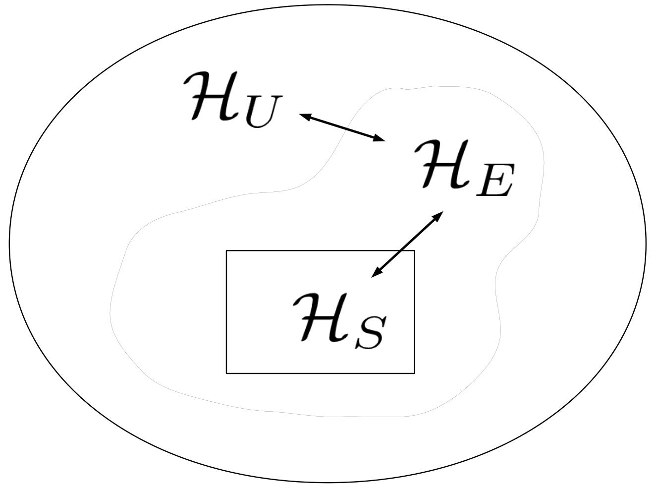
Eqn. (1) also includes terms that allow our environment to be coupled to the rest of the universe denoted by ${\cal H}_{U}$. When such a wider environment is present, we assume that it is well approximated by an infinite heat bath that is kept in a thermal state. The oscillator modes of the immediate environment are then dynamically driven towards a thermal state by virtue of the environment to universe coupling term ${\cal H}_{EU}$. However, unlike conventional Born-Markov weak coupling approaches which commonly keep the entire environment fixed in thermal equilibrium, the inner tier modes will in general deviate from the thermal state. We shall show this adds an exponential cut-off to the response kernel. Figure 1 gives an illustration of our model.

Instead of explicitly treating the coupling between the environment and the rest of the universe with a microscopic derivation, we make the simplifying assumption that ${\cal H}_{EU}$ is small enough that each mode $\omega_{k}$ of the environment simply experiences damping with rate $\gamma_{k}$ via standard Lindblad operators (for a derivation see, e.g., Ref. 5). For this to be consistent, two conditions must be satisfied: Firstly, the damping rate $\gamma_{k}\ll\omega_{k}$ must be small for each mode, because this is the parameter regime assumed in the derivation of the damped harmonic oscillator master equation. Secondly, the system-environment coupling described by ${\cal H}_{I}$ may not become too large either,

otherwise the damping Lindblad operators acting on each mode are influenced by the presence of the system and our simple independent choice ceases to be a good approximation [51] (also see Ref. 15 for a discussion of this approximation in the context of the resonant damped Jaynes-Cummings model).

Finally, we assume that the initial density matrix can be factorized as $\rho(0)=\rho_{s}(0)\otimes\rho_{E}^{th}$ with the initial thermal state of the environment being $\rho_{E}^{th}={\cal N}^{-1}\exp(-\beta{\cal H}_{E})$ (where ${\cal N}$ is the appropriate normalization factor).

To represent the density matrix of a single harmonic oscillator we use the coherent state or P representation[52], which has been extensively studied in quantum optics. The coherent state representation maps between the density matrix of a harmonic oscillator $\rho$ and a function of two continuous variables $P(\alpha,\alpha^{*})$ via

where $\left|\alpha\right\rangle$ is the coherent state defined as $\left|\alpha\right\rangle=e^{\alpha a^{\dagger}-\alpha^{*}a}\left|0\right\rangle$ or alternatively $a\left|\alpha\right\rangle=\alpha\left|\alpha\right\rangle$, and $d^{2}\alpha\equiv d\text{Re}(\alpha)d\text{Im}(\alpha)$. The mapping yields the following operator correspondence [52]:

For a system with states $\left|i\right\rangle$ coupled to an oscillator, instead of a $P$ function we now need a $P$ matrix to represent the density matrix,

Generalizing from a single mode to a set of modes is straightforward, with the corresponding set of variables $\{a_{k},a^{\dagger}_{k}\}\leftrightarrow\{\alpha_{k},\alpha^{*}_{k}\}$ and

A partial trace over the oscillator space is given by

For notational ease, from hereon we switch to a vectorized form of the density matrix and operators, mapping $n\times n$ matrices $A_{i,j}$ to vectors ${A_{i}}$ of dimension $n^{2}$. Further, we use the generalized Gell-Mann matrices with the notation from Ref. 53. For an $n$-site system, these consist of $n^{2}-1$ traceless and Hermitian matrices $\nu_{1},\nu_{2},\cdots,\nu_{n^{2}-1}$, defining a full operator basis together with the identity matrix.¹¹ 1 For $n=2$ (a qubit) $\nu_{i}=\sigma_{i}$ are the Pauli matrices, and for $n=3$ we get the Gell-Mann matrices $\nu_{i}=\lambda_{i}$. Adopting the Einstein summation convention, where $i,j,k$ run from $1$ to $n^{2}-1$, the generalized Gell-Mann matrices satisfy:

where $f_{ijk}$ and $d_{ijk}$ are totally antisymmetric and symmetric tensors, respectively. For $n=2,f_{ijk}=\epsilon_{ijk}$ the Levi-Civita symbol and $d_{ijk}=0$. Any $n\times n$ matrix $P$ can be written as a vector $P_{i}$:

Using this vectorized form we can write the density matrix as

where for convenience we denote $\int_{\alpha}\equiv\prod_{k}\int d^{2}\alpha_{k}$, and $P=P(\{\alpha_{k},\alpha^{*}_{k}\})$. The condition $Tr\rho=1$ implies $\int d^{2}\alpha P_{n^{2}}(\alpha,\alpha^{*})=1/n$, and we are interested in the partial trace over the environment

At this stage, we use the following form for writing down the full dynamics of the reduced system:

where $U(t)$ is the propagator (in the vectorized representation) of the system without the environment, and the influence of the rest of the world on the system is encoded in the influence functional $\Theta(t)$. The motivation for this comes from the Feynman-Vernon influence functional [55] of the same form. Further, we anticipate that this form will be a convenient one for recovering the known exponential decay in the weak-coupling limit. The main result of this paper is that it is possible to find an exact expansion of $\Theta(t)$ as a perturbation series with respect to the interaction ${\cal H}_{I}$, and expansion up to second order recovers the known dephasing and relaxation rates given by standard Born-Markov weak master-equation techniques, but with an added non-Markovian contribution.

For the perturbation treatment, we use the expansion

hence Eqn. (23) translates to:

The solution for the uncoupled system $P^{0}$ is simply given by

with $\rho^{s}(t)=[\rho^{s}_{1}(t),\rho^{s}_{2}(t),\dots,\rho^{s}_{n^{2}-1}(t),1/n]$. In principle it is possible to solve this series term by term. However, we are interested in the state of the system and not the oscillator, which makes things much easier: We use the boundary condition where $\alpha^{k}P^{n}(\alpha)\underset{\alpha\rightarrow\infty}{\longrightarrow}0$ for all $k,n$. This is justified since the oscillator can be expected not to deviate by too much from a thermal, Gaussian state, and it certainly also should not occupy extreme high-energy states. Therefore performing the integration $\int d^{2}\alpha\equiv\int_{\alpha}$ on Eqn. (35-37) yields

where

is the matrix equivalent to the superoperator $[V,\square]$. The initial condition is $\int_{\alpha}P^{n>0}(t=0)=0$, i.e. at time $t=0$ the qubit and the mode are factorized, and the mode is in the thermal state, which gives

for all times. The first contribution in the expansion therefore comes from $\int_{\alpha}P^{2}(\alpha,t)\neq 0$, which is $2^{nd}$ order in the coupling constant $g$. This is in analogy to the usual QME treatment, where the influence of the environment also enters at the $2^{nd}$ order in the coupling constant. In order to solve Eqn. (40) we first need to evaluate $\int_{\alpha}(\alpha+\alpha^{*})P^{1}$, which can be done by invoking the following mathematical procedure: (i) multiply Eqn. (35) by $\alpha$ or $\alpha^{*}$ from the left; (ii) perform the $\int_{\alpha}$ integral; (iii) integrate by parts all terms possessing a derivative. The sequence of these steps yields the following two equations:

which after a bit of algebra and ODE solving yield a solution for $\int_{\alpha}P^{1}$. Substituting this solution into Eqn. (40) then results in

Here, the notation $\tilde{V}^{\times},\tilde{V}^{\circ}$ denotes operators in the Heisenberg picture,

and $\tilde{V}^{\circ}$ is the equivalent of $\{V,\Box\}$ and is given by

At this point we note that the influence functional $\Theta(t)$ up to second-order in $g$ is then given by Eqn. (47) and

We proceed by showing that this provides a highly accurate solution for the single mode case in the weak-coupling limit. We shall then generalise the technique to an environment consisting of a (quasi)continuous bath of oscillators. In Appendix B we sketch the derivation of higher-order terms in the perturbation series.

The Rabi model, consisting of a coupled 2LS to a harmonic oscillator, represents perhaps the most basic and ubiquitous compound quantum system. Focussing only on the dynamics of the 2LS and tracing over the oscillator then results in arguably the conceptually most simple and yet a highly non-trivial open systems problem. Let us consider the Rabi Hamiltonian

where $\sigma_{i}$ are the usual Pauli matrices referring to the 2LS. In this case, we immediately find that the matrices ${\cal H}_{S}^{\times},V^{\times},V^{\circ}$ are given by:

when operating on the vector $\{\sigma_{x},\sigma_{y},\sigma_{z},{\hbox{1\kern-1.49994pt\vrule width=0.8pt,depth=-0.5pt}}\}^{\dagger}$. Substituting these into Eqn. (53), we obtain an unwieldy analytical expression for $\Theta(t)$, which can give us insight if examined in the eigenbasis of the system (the ${\cal H}_{S}^{\times}$ eigenbasis): the top $3\times 3$ part of ${\cal H}_{S}^{\times}$ has two finite and one vanishing eigenvalue ($\{0,\pm\sqrt{\epsilon^{2}+\Delta^{2}}\}$). In this basis, the real terms on the diagonal of $\Theta(t)$ that are proportional to $t$ and correspond to the finite eigenvalues, are both equal to the dephasing rate. The one corresponding to the vanishing eigenvalue is the relaxation rate. These rates are given by

where $\Omega=\sqrt{\epsilon^{2}+\omega^{2}}$ is the Rabi frequency. Note that in the limit $\gamma\rightarrow 0$, i.e. no damping on the oscillator from the wider environment or universe, we recover the standard Born-Markov ME result for relaxation and dephasing, given in Eqns. (127-128). The imaginary parts on the diagonal of $\Theta(t)$ correspond to the Lamb shift Hamiltonian, given by

where $\tilde{\sigma_{z}}$ is given by writing the system Hamiltonian, i.e. the first two terms in Eqn. (54) in its diagonal basis

Again, in the limit $\gamma\rightarrow 0$ we recover the “standard” Lamb shift given in Eqn. (123). Furthermore, we can extract the steady state of the system at long times: At times much larger than the relaxation time, the system tends to the state

This is indeed only the expected thermal system state when $\gamma\rightarrow 0$ and $\omega\rightarrow\Omega$, i.e. no damping and when oscillator and system are resonant. However, one should take this limit with caution, because for vanishing damping, $\gamma\rightarrow 0$ the relaxation time $\Gamma_{\text{relax}}^{-1}$ tends to infinity and the system will thus never actually reach this state. In Fig. 2 we plot the effective temperature, that is, the temperature $T_{\text{eff}}$ given by equating $\exp[-\tilde{{\cal H}}_{S}/k_{b}T_{\text{eff}}]$ with Eqn. (62). On the same figure we plot the relaxation rate for the same parameters, showing a Lorentzian peak in efficiency near resonance.

We note that in general the effective temperature differs from the temperature of the universe. In order to explain this apparent discrepancy, we examine Eqn. (62): The universe is only directly coupled to the oscillator which has energy levels spacing of $\omega$, this accounts for the term $\tanh(\frac{\beta\omega}{2})$ which is different from the expected $\tanh(\frac{\beta\Omega}{2})$. This term decreases (increases) the effective temperature $T_{\text{eff}}$ when the mode is blue-shifted (red-shifted) with respect to the Rabi frequency $\Omega$. The pre-factor

is maximized when on resonance ($\omega=\Omega$). Detuning suggests that in order to extract energy from the qubit, the universe exchanges energy with the oscillator to match the detuning. This adds uncertainty to the system effectively increasing the temperature. The system-environment coupling $\gamma$ adds additional uncertainty.

We also note that in this scheme we do not keep track of the environment, only trace over it. The thermal state of system+environment is proportional to $\exp[-\beta({\cal H}_{S}+{\cal H}_{E}+{\cal H}_{I})]$, i.e. the system and environment are entangled, and defining a temperature of just one subsystem is questionable.

The example we discuss in this section is formally equivalent to the reaction coordinate [18, 19, 20] or structured environment [21, 22, 23, 24] model in the weak coupling and weak damping regime. Here, the reaction coordinate model employs an effective spectral density with a Lorenzian peak, yielding the same rates as Eqns. (58-60) except for the “counter rotating” terms $\sim(\Omega+\omega)^{-n}$ (which are typically small). Interestingly however, this nice agreement only extends to the real part of the response function, $D(t)$, which determines the damping rates. By contrast, the modified spectral density of the reaction coordinate method does not account for corrections to the imaginary part $D_{1}(t)$, which yields the long time asymptotic behaviour of the system. To ensure that our approach does indeed deliver the correct steady state, we have made a comparison with an exact numerical simulation of the dynamics given by Hamiltonian (54) (with ${\cal H}_{EU}+{\cal H}_{U}$ replaced by a Lindblad dissipator). We obtain perfect agreement between Eqn. (62) and a purely numerical simulation in the weak coupling regime.

In Figure 3 we plot a comparison between Eqn. (18) with $\Theta(t)$ approximated by Eqn. (53), and exact numerical simulation, showing that for the weak-coupling regime there is a very good agreement between the two.

To apply our generalized multimode technique to a particular example, we look at the well studied case of the (biased) spin-boson model with the following Hamiltonian:

In this case, just like for the Rabi model, the system is two-dimensional and its P vector has 4 components ($\sigma_{x},\sigma_{y},\sigma_{z},{\hbox{1\kern-1.49994pt\vrule width=0.8pt,depth=-0.5pt}}$), and ${\cal H}_{S}^{\times},V^{\times},V^{\circ}$ are again given by Eqns. (55-57). Since we have already calculated the relaxation and dephasing rates for the single mode case, showing that the different modes contribute independently for $\Theta(t)$ in the weak-coupling regime, we can immediately write down the following expressions for the relaxation rates: we only need to add a summation $\sum_{k}$ over the different modes to Eqns. (58-59):

We note that, as discussed at the end of Section IV, in the limit of $\gamma_{k}\rightarrow 0$, we recover the known weak-coupling rates, cf. Ref. 56 or Appendix C. The second part of Eqn. (74) is known as the pure dephasing constant.

Below we study the no-bias case, setting $\epsilon=0$: the system Hamiltonian (${\cal H}_{S}^{\times}$ in our language) is static, hence the propagator $U$ is given by $U=\exp[-i{\cal H}_{S}^{\times}t]$. To calculate $\Theta(t)$, we can make a change of variables in the double integral $\int_{0}^{t}dt^{\prime}\int_{0}^{t^{\prime}}dt^{\prime\prime}=\int_{0}^{t}d\tau\int_{\tau/2}^{t-\tau/2}d\eta$ to get the expression:

with

In the above expression, $\Theta_{\text{relax}}$ induces the relaxation and decoherence, $\Theta_{\text{LS}}$ induces the Lamb-shift, and $\Theta_{\text{th}}$ steers the system towards the thermal state. $\Theta_{\text{RW}}$ is usually ignored under the rotating wave approximation. If one is interested in times $t\gg\tau_{b}$ much longer than the memory of the bath $D(t>\tau_{b})\rightarrow 0$, it is justified to let the upper limit of the integrals go to infinity. For this case it is most insightful to examine this result in light of the standard quantum-optical master equation approach: In the standard approach, remarkably one gets exactly the same expressions as the above Eqn. (75) [without Eqn. (79)], but with an interesting change:

The terms which are not proportional to $t$ capture non-Markovian contributions, giving information about the bath’s reorganization time. Interestingly, each of the environmental effects possesses its own timescale, and these are estimated by

It is noteworthy that the reorganization times can be negative. This could happen when, for example, initially for $t\lesssim\tau_{b}$ the dephasing process, which includes a non-Markovian component, is more aggressive than at later times when it assumes a stable value. Then, as the aggressive decay stops, the population of the system has fallen by a greater amount than it would have done under the stable, long lived decay process. Thus the system appears as if it has been evolving under the stable dephasing rate for a longer time than it actually has, and hence the negative reorganization time. We note that the terms (81-83) in the limit $\gamma\rightarrow 0$ are known in the literature as those leading to the slippage of initial conditions, and are important for preserving the positivity of the reduced density matrix.[57, 58]

The steady-state of the system is given by

A comparison between the standard Markovian Master equation, the current method and exact numerical simulation for the case of a super-Ohmic environment is shown in Fig. 4. The QUAPI technique [6, 7, 8] is used as an exact numerical benchmark curve: Our calculation uses nine kernel time steps, covering a total kernel memory time of 2 ps and is fully converged. The standard Born-Markov weak-coupling approach is given in Appendix C. Clearly, our method’s non–Markovian nature and lack of Born approximation results in an impressive improvement over the standard Born-Markov weak coupling ME approach. For this particular comparison, since there is no wider universe involved, $\gamma(\omega)=0$, the current method is equivalent to the second-order TCL approach, which also does not employ any approximations beyond a perturbation in the system-environment coupling. However, a key strength of the current formulation is that it is trivial to include a wider universe, which simply enters in the form of an exponential cut–off to the response function.

We note that this method allows us to easily study the case where the spectral density has several discrete sharp peaks as well as a smooth background, which is believed to be the case in many (if not all) systems studied in quantum biology [60, 10]. In this case the response function vanishes very slowly, which makes an exact numerical treatment extremely demanding, as a long history of the system needs to be tracked. In some papers, such as Ref. 60 this issue is resolved by approximating a delta-function peak in the spectral density as a Lorentzian with a finite width. We note that if one allows this single peak to be damped, then in light of Eqn. (62), this mode drives the system to an effective temperature different from the initial temperature of the environment $T$. Hence replacing discrete modes with Lorentzian distributions added to a continuous spectral density may in some parameters regimes become a questionable approximation. By contrast, the additive property of modes to the influence functional $\Theta(t)$ here allows us to combine a discrete set of modes with a smooth background by taking

As an example for this, let us study the spin boson model with a smooth background of oscillators plus a more strongly coupled discrete peak of frequency $\omega_{s}$ in the environment. We single out this peak and label it henceforth with a subscript $s$, writing the system-environment Hamiltonian as

References

- [1] G. S. Engel, T. R. Calhoun, E. L. Read, T. Ahn, T. Mancal, Y. Cheng, R. E. Blankenship, and G. R. Fleming, “Evidence for wavelike energy transfer through quantum coherence in photosynthetic systems.” Nature 446, 782–6 (2007).
- [2] E. Collini, C. Y. Wong, K. E. Wilk, P. M. G. Curmi, P. Brumer, and G. D. Scholes, “Coherently wired light-harvesting in photosynthetic marine algae at ambient temperature,” Nature 463, 644–647 (2010).
- [3] J. Cai, G. G. Guerreschi, and H. J. Briegel, “Quantum control and entanglement in a chemical compass,” Phys. Rev. Lett. 104, 220502 (2010).
- [4] E. M. Gauger, E. Rieper, J. J. L. Morton, S. C. Benjamin, and V. Vedral, “Sustained Quantum Coherence and Entanglement in the Avian Compass,” Physical Review Letters 106, 040503 (2011).
- [5] H. P. Breuer and F. Petruccione, The Theory of Open Quantum Systems (Clarendon Press, 2007).
- [6] N. Makri, “Improved Feynman propagators on a grid and non-adiabatic corrections within the path integral framework,” Chemical Physics Letters 193, 435–445 (1992).
- [7] N. Makri and D. E. Makarov, “Tensor propagator for iterative quantum time evolution of reduced density matrices. II. Numerical methodology,” The Journal of Chemical Physics 102, 4611 (1995a).
- [8] N. Makri and D. E. Makarov, “Tensor propagator for iterative quantum time evolution of reduced density matrices. I. Theory,” The Journal of Chemical Physics 102, 4600 (1995b).
- [9] P. Nalbach, J. Eckel, and M. Thorwart, “Quantum coherent biomolecular energy transfer with spatially correlated fluctuations,” New Journal of Physics 12, 065043 (2010).
- [10] P. Nalbach, D. Braun, and M. Thorwart, “Exciton transfer dynamics and quantumness of energy transfer in the Fenna-Matthews-Olson complex,” Physical Review E 84, 041926 (2011).
- [11] H. P. Breuer, “Genuine quantum trajectories for non-Markovian processes,” Physical Review A 70, 012106 (2004).
- [12] A. Imamoglu, “Stochastic wave-function approach to non-Markovian systems,” Physical Review A 50, 3650–3653 (1994).
- [13] H. Gassmann, F. Marquardt, and C. Bruder, “Non-Markoffian effects of a simple nonlinear bath,” Physical Review E 66, 041111 (2002).
- [14] G. Katz, D. Gelman, M. a Ratner, and R. Kosloff, “Stochastic surrogate Hamiltonian.” The Journal of chemical physics 129, 034108 (2008).
- [15] M. Scala, B. Militello, A. Messina, J. Piilo, and S. Maniscalco, “Microscopic derivation of the Jaynes-Cummings model with cavity losses,” Physical Review A 75, 013811 (2007).
- [16] M. M. Wolf and J. I. Cirac, “Dividing quantum channels,” Communications in Mathematical Physics 168, 147–168 (2008).
- [17] B. J. Dalton, S. M. Barnett, and B. M. Garraway, “Theory of pseudomodes in quantum optical processes,” Physical Review A 64, 053813 (2001).
- [18] A. Garg, J. N. Onuchic, and V. Ambegaokar, “Effect of friction on electron transfer in biomolecules,” The Journal of Chemical Physics 83, 4491 (1985).
- [19] M. Thorwart, L. Hartmann, I. Goychuk, and P. Hänggi, “Controlling decoherence of a two-level-atom in a lossy cavity,” Journal of Modern Optics 47:14-15, 2905–2919 (2000), arXiv:0003029 [quant-ph] .
- [20] K. H. Hughes, C. D. Christ, and I. Burghardt, “Effective-mode representation of non-Markovian dynamics: a hierarchical approximation of the spectral density. II. Application to environment-induced nonadiabatic dynamics.” The Journal of chemical physics 131, 124108 (2009).
- [21] M. Thorwart, E. Paladino, and M. Grifoni, “Dynamics of the spin-boson model with a structured environment,” Chemical Physics 296, 333–344 (2004).
- [22] M. Goorden, M. Thorwart, and M. Grifoni, “Entanglement Spectroscopy of a Driven Solid-State Qubit and Its Detector,” Physical Review Letters 93, 267005 (2004).
- [23] M. C. Goorden, M. Thorwart, and M. Grifoni, “Spectroscopy of a driven solid-state qubit coupled to a structured environment,” The European Physical Journal B 45, 405–417 (2005).
- [24] P. Huang and H. Zheng, “Quantum dynamics of a qubit coupled with a structured bath,” Journal of Physics: Condensed Matter 20, 395233 (2008).
- [25] D. Rossini, T. Calarco, V. Giovannetti, S. Montangero, and R. Fazio, “Decoherence induced by interacting quantum spin baths,” Physical Review A 75, 032333 (2007), arXiv:0611242 [quant-ph] .
- [26] M. P. Woods, R. Groux, A. W. Chin, S. F. Huelga, and M. B. Plenio, “Mappings of open quantum systems onto chain representations and Markovian embeddings,” Journal of Mathematical Physics 55, 032101 (2014).
- [27] Y. Tanimura and R. Kubo, “Time evolution of a quantum system in contact with a nearly Gaussian-Markoffian noise bath,” Journal of the Physical Society of Japan 58, 101–114 (1989).
- [28] Y. Tanimura, “Nonperturbative expansion method for a quantum system coupled to a harmonic-oscillator bath,” Physical Review A 41, 6676–6687 (1990).
- [29] Y. Tanimura and P. G. Wolynes, “Quantum and classical Fokker-Planck equations for a Gaussian-Markovian noise bath,” Physical Review A 43, 4131–4142 (1991).
- [30] A. Ishizaki and G. R. Fleming, “Unified treatment of quantum coherent and incoherent hopping dynamics in electronic energy transfer: reduced hierarchy equation approach.” The Journal of Chemical Physics 130, 234111 (2009a).
- [31] A. Ishizaki and G. R. Fleming, “Theoretical examination of quantum coherence in a photosynthetic system at physiological temperature.” Proceedings of the National Academy of Sciences of the United States of America 106, 17255–60 (2009b).
- [32] N. Makri, “Numerical path integral techniques for long time dynamics of quantum dissipative systems,” Journal of Mathematical Physics 36, 2430–2457 (1995).
- [33] A. Ishizaki and Y. Tanimura, “Quantum Dynamics of System Strongly Coupled to Low-Temperature Colored Noise Bath: Reduced Hierarchy Equations Approach,” Journal of the Physics Society Japan 74, 3131–3134 (2005).
- [34] D. Süß, A. Eisfeld, and W. T. Strunz, “Hierarchy of stochastic pure states for open quantum system dynamics,” Physical Review Letters 113, 150403 (2014), arXiv:1402.4647 .
- [35] J. Roden, W. T. Strunz, and A. Eisfeld, “Non-markovian quantum state diffusion for absorption spectra of molecular aggregates.” The Journal of Chemical Physics 134, 034902 (2011).
- [36] L. Diósi and W. T. Strunz, “The non-Markovian stochastic Schrödinger equation for open systems,” Physical Letters A 235, 569–573 (1997).
- [37] L. Diósi, N. Gisin, and W. T. Strunz, “Non-Markovian quantum state diffusion,” Physical Review A 58, 1699–1712 (1998).
- [38] G. Ritschel, J. Roden, W. T. Strunz, and A. Eisfeld, “An efficient method to calculate excitation energy transfer in light-harvesting systems: application to the Fenna–Matthews–Olson complex,” New Journal of Physics 13, 113034 (2011).
- [39] M. J. Burek, D. Ramos, P. Patel, I. W. Frank, and M. Lončar, “Nanomechanical resonant structures in single-crystal diamond,” Applied Physics Letters 103, 131904 (2013).
- [40] O. Arcizet, V. Jacques, A. Siria, P. Poncharal, P. Vincent, and S. Seidelin, “A single nitrogen-vacancy defect coupled to a nanomechanical oscillator,” Nature Physics 7, 879–883 (2011).
- [41] M. Ganzhorn, S. Klyatskaya, M. Ruben, and W. Wernsdorfer, “Strong spin-phonon coupling between a single-molecule magnet and a carbon nanotube nanoelectromechanical system.” Nature nanotechnology 8, 165–9 (2013).
- [42] A. Pályi, P. R. Struck, M. Rudner, K. Flensberg, and G. Burkard, “Spin-Orbit-Induced Strong Coupling of a Single Spin to a Nanomechanical Resonator,” Physical Review Letters 108, 206811 (2012).
- [43] J. Chan, T. P. M. Alegre, A. H. Safavi-Naeini, J. T. Hill, A. Krause, S. Gröblacher, M. Aspelmeyer, and O. Painter, “Laser cooling of a nanomechanical oscillator into its quantum ground state.” Nature 478, 89–92 (2011).
- [44] M. D. LaHaye, J. Suh, P. M. Echternach, K. C. Schwab, and M. L. Roukes, “Nanomechanical measurements of a superconducting qubit.” Nature 459, 960–4 (2009).
- [45] C. Eichler, C. Lang, J. M. Fink, J. Govenius, S. Filipp, and A. Wallraff, “Observation of entanglement between itinerant microwave photons and a superconducting qubit,” Phys. Rev. Lett. 109, 240501 (2012).
- [46] J. M. Pirkkalainen, S. U. Cho, J. Li, G. S. Paraoanu, P. J. Hakonen, and M. A. Sillanpää, “Hybrid circuit cavity quantum electrodynamics with a micromechanical resonator.” Nature 494, 211–5 (2013).
- [47] E. J. O’Reilly and A. Olaya-Castro, “Non-classicality of the molecular vibrations assisting exciton energy transfer at room temperature.” Nature communications 5, 3012 (2014).
- [48] J. Prior, A. W. Chin, S. F. Huelga, and M. B. Plenio, “Efficient simulation of strong system-environment interactions,” Phys. Rev. Lett. 105, 050404 (2010).
- [49] J. Iles-Smith, N. Lambert, and A. Nazir, “Environmental dynamics, non-Gaussianity, and the emergence of noncanonical equilibrium states in open quantum systems,” Physical Review A 90, 032114 (2014).
- [50] A. Fruchtman et al., manuscript in preparation (2014).
- [51] H. J. Carmichael and D. F. Walls, “Master equation for strongly interacting systems,” Journal of Physics A: Mathematical, Nuclear and General 6, 1552 (1973).
- [52] C. Gardiner and P. Zoller, Quantum Noise: A Handbook of Markovian and Non-Markovian Quantum Stochastic Methods with Applications to Quantum Optics, Springer Series in Synergetics (Springer, 2004).
- [53] A.J. Macfarlane, A. Sudbery, and P.H. Weisz, “On Gell-Mann’s -matrices, and tensors, octets, and parametrizations of SU(3),” Communications in Mathematical Physics 11, 77–90 (1968).
- [54] For (a qubit) are the Pauli matrices, and for we get the Gell-Mann matrices .
- [55] R. P. Feynman and F. L. Vernon, “The theory of a general quantum system interacting with a linear dissipative system,” Annals of Physics 173, 118–173 (1963).
- [56] U. Weiss, Quantum Dissipative Systems, Vol. 13 (World Scientific, 2012).
- [57] A. Suárez, R. Silbey, and I. Oppenheim, “Memory effects in the relaxation of quantum open systems,” The Journal of Chemical Physics 97, 5101 (1992).
- [58] P. Gaspard and M. Nagaoka, “Slippage of initial conditions for the Redfield master equation,” The Journal of Chemical Physics 111, 5668 (1999).
- [59] D. P. S. McCutcheon, N. S. Dattani, E. M. Gauger, B. W. Lovett, and A. Nazir, “A general approach to quantum dynamics using a variational master equation: Application to phonon-damped Rabi rotations in quantum dots,” Physical Review B 84, 081305 (2011).
- [60] C. Kreisbeck and T. Kramer, “Long-Lived Electronic Coherence in Dissipative Exciton Dynamics of Light-Harvesting Complexes,” The Journal of Physical Chemistry Letters 3, 2828–2833 (2012).
- [61] R. Graham and M. Höhnerbach, “Two-state system coupled to a boson mode: quantum dynamics and classical approximations,” Zeitschrift für Physik B Condensed Matter 248, 233–248 (1984).
- [62] F. A. Pollock, D. P. S. McCutcheon, B. W. Lovett, E. M. Gauger, and A. Nazir, “A multi-site variational master equation approach to dissipative energy transfer,” New Journal of Physics 15, 075018 (2013).
- [63] K. D. B. Higgins, B. W. Lovett, and E. M. Gauger, “Quantum thermometry using the ac Stark shift within the Rabi model,” Phys. Rev. B 88, 155409 (2013).