Stability of an upwind Petrov-Galerkin discretization of convection diffusion equations
Abstract
We study a numerical method for convection diffusion equations, in the regime of small viscosity. It can be described as an exponentially fitted conforming Petrov-Galerkin method. We identify norms for which we have both continuity and an inf-sup condition, which are uniform in mesh-width and viscosity, up to a logarithm, as long as the viscosity is smaller than the mesh-width or the crosswind diffusion is smaller than the streamline diffusion. The analysis allows for the formation of a boundary layer.
Introduction
For many fluid flow problems of relevance to engineering, the convective term, hyperbolic in nature, is moderated by a viscous term, elliptic in nature. For large viscosity, Galerkin finite element methods yield good results. As the viscosity tends to zero, sharp gradients in the fluid velocity as well as boundary layers will appear. When the characteristic length of boundary layers is smaller than the mesh-width, standard Galerkin methods become unstable. This prominent example of a multiscale problem has motivated a large body of work on stabilised methods. For overviews and introductions we refer to [10] and [9].
This paper is motivated by a general method, introduced in [6], that applies to differential forms on arbitrary meshes. It produces differential complexes of finite element spaces that take into account convection. It treats uniformly differential -forms of all degrees . Thus it fits into the framework of finite element exterior calculus (FEEC) [2]. More precisely it fits into the framework of finite element systems (FES) [5], which was designed to accommodate polyhedral meshes and quite general basis functions, yet produce discrete spaces equipped with commuting interpolators. So far we have not provided any analysis of this method in the convection dominated regime, even for scalar problems.
For scalar equations on product grids, the method relates to exponential fitting. Variants of exponential fitting can be traced all the way back to [1] and [12]. This method can be analysed quite exhaustively in dimension one, for instance because, in model situations, the discrete solution turns out to interpolate the exact one at vertices. However, already in dimension two, in spite of its naturality, the method is hard to analyse, compared with Galerkin methods at large viscosity.
To be more precise, one defines upwinded finite elements that solve local problems related to the adjoint equation. Downwinded elements, on the other hand, locally solve problems related to the original equation. In cases where these problems can be solved explicitly one often obtains exponential functions with viscosity dependent parameters, hence the name. In [8] a Galerkin method with downwinded elements is analysed. We, on the other hand, are interested in a Petrov-Galerkin method with a standard trial space, and an upwinded test space. Compared with for instance [7] we point out that our methods produce conforming spaces.
One of our main sources of inspiration for our stability proof is [3]. This paper analyses a parabolic problem with an -norm in time. For our purposes the time-variable corresponds to a space-variable which increases in the direction of the flow. The Hilbert transform, which provides an inf-sup estimate for the convective term, plays a prominent role in our arguments. Many of our arguments use, in intermediate steps, a slightly weaker variant of , a certain critical Besov space containing discontinuous functions. Both projection onto piecewise constants and interpolation onto upwinded functions behave quite well in this norm, as we show.
We point out that also [11] advocates the use of a -norm for convection diffusion problems. The theory of that paper pertains to a posteriori estimates for one-dimensional problems, but numerical results are reported also for multi-dimensional problems. In [4] an anisotropic -norm is also considered, in a multi-dimensional setting. The numerical methods analysed in [4] and [11] (Fourier/Wavelets and SUPG respectively) are quite different from the one we consider here.
For a certain choice of viscosity dependent norms, essentially the anisotropic -norm plus the energy norm, we prove both a continuity estimate and an inf-sup condition, for the discrete method, up to a logarithmic factor in the viscosity. Admittedly the hypothesis required for our proof, essentially that the flow is aligned with the mesh, is very restrictive. On the other hand, we do prove stability under hypotheses that allow for the formation of a boundary layer at the outflow boundary. It is our hope that the paper might give a reasonable idea of what sort of arguments should be improved upon to handle more realistic meshes.
The paper is organized as follows. In §1 we set up the model problem we consider and discuss some numerical results. In §2 we provide a study, based on [3], of some parabolic problems, to motivate our techniques. In §3 we provide continuity estimates, in the norms of interest, for some operators acting on functions of one real variable, in particular projection onto piecewise constants and the nodal interpolator, acting from piecewise affines to upwinded functions. In §4 we put our results together to prove an inf-sup condition for convection diffusion problems. An appendix contains our first proof of this result, which was more cumbersome.
1 Problem setup
We consider a domain in . On this domain we consider the equation:
| (1) |
The scalar is constant in the domain and will be referred to as viscosity. The vector field , responsible for convection, is also constant in the domain, and directed along the first axis. With a slight abuse of notations we take it of the form for a scalar and the unit vector along the fist axis. The function is bounded and non-negative. The right hand side is given in . We impose homogeneous Dirichlet conditions on . This equation has a unique solution in , as can be deduced from the Lax-Milgram lemma.
We are interested in letting the parameter tend to , all other data remaining fixed. If we let denote the corresponding solution, we know that converges in to some function as tends to . It then follows that:
| (2) |
In general therefore the -seminorm of blows up. One observes the formation of a boundary layer at the outflow boundary, which is the part of where , where denotes the outward pointing normal vector on . A boundary layer of a rather different nature appears close to the part of the boundary where . Away from the boundary layers, converges to in strong norms. The limit satisfies the homogeneous boundary condition on the inflow boundary (where ), but in general not elsewhere.
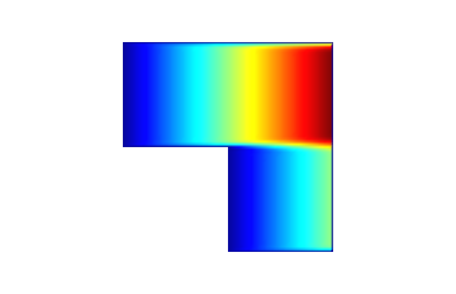

In Figure 1 numerical results are shown for , and . The width of the domain in the horizontal direction is 1. We chose . The standard numerical method we use, is a Galerkin finite element method with continuous finite elements on a square grid of width . For we observe that the numerical solution is very oscillatory (right hand figure). This well-known instability appears whenever the Péclet number exceeds 1 (for the displayed figure it is above 40). The upwinded method we propose is a Petrov-Galerkin method with as trial space and a test space we now proceed to describe.
Generally speaking, consider a mesh consisting of cells of various dimensions: vertices (dimension ), edges (dimension ), faces (dimension ), etc. arranged in a cellular complex. For definiteness one can think of simplicial complexes or product grids. Actually only the latter are considered in our numerical experiments and for the stability proof we present in the following sections.
For each cell , of any dimension, let be the tangential component of on . We construct an upwinded basis function attached to a given vertex by first assigning the value 1 to this vertex, and the value 0 to all others. Next we extend recursively, from vertices to edges, from edges to faces, etc, each time solving the equation, on say the cell (with prescribed boundary values):
| (3) |
We may remark that if the method of recursive harmonic extension produces the piecewise affines on simplicial meshes, and the tensor product functions on orthogonal product meshes. On such meshes the obtained functions are simple also in the case where is non-zero (but constant on the domain): On an edge the solutions to (3) are linear combinations of the constant function and a certain exponential:
| (4) |
If one replaces of course the exponential by a linear function. Globally one obtains, from the recursive extension procedure, tensor products of such functions.
We develop our theory for the case when the domain is of the form and the mesh is aligned with the first axis, which is also the direction of the vector field . In this case we obtain, with the above method, the tensor products of functions which in the direction of the first axis are piecewise of the form (4), and which in the direction of are standard functions. This defines our upwinded test space. Recall that the trial space is just .
For applications it is important that the numerical method be able to treat variable , not necessarily aligned with the mesh. This is done by replacing (3) by :
| (5) |
and solving this equation approximately on a sub-grid. The particular sub-grid we advocate consists in adding one point to each cell of the mesh, and taking the corresponding simplicial refinement. The added points are placed taking into account the expected singular behaviour of the upwinded basis functions. In other words we do a barycentric refinement, where barycenters are computed with weights involving the Péclet number . The main reason for preferring (5) to (3) is that in this form the discrete upwinding method (involving typically an adapted subgrid) extends nicely to differential forms, as explained in [6].
In Figure 2 we have plotted the relative distance between the numerical solutions and obtained with exact and approximate upwinding respectively, with respect to the norm defined by:
| (6) |
We first notice that the relative error stays below 0.03 in this experiment, indicating that the use of approximate unwinding does not change too much the computed solution. In the following sections we just analyse the case of exact upwinding.
Interestingly, we also notice that the relative error, between exact and discrete upwinding in the computed solutions, seems to be maximal along a certain line, here given by . We also noticed that the relative error between the exact and upwinded basis functions is maximal along such a line, but with a different proportionality constant.
2 A study of parabolic problems
In this section we give our reading of [3]. It serves mainly to motivate the techniques of the next sections. Some improvements occur, because in our setting the viscosity is destined to become small, as illustrated by Lemma 2.3. We shall restrict our attention to the Crank-Nicolson scheme, whereas [3] treats some other discretizations as well.
Inf-Sup condition.
We state some ways in which inf-sup conditions may be obtained, for bilinear forms on Hilbert spaces.
Proposition 2.1.
Suppose and are Hilbert spaces and that is a continuous bilinear form. Suppose we have a continuous linear map such that:
| (7) | ||||
| (8) |
Then satisfies the inf-sup condition:
| (9) |
Proof.
For non-zero we have and we may write:
| (10) |
The inf-sup estimate follows. ∎
Proposition 2.2.
Suppose we have two Hilbert spaces and , and two continuous bilinear forms and on . Suppose we have two continuous operators and from to such that for some :
| (11) |
Suppose moreover that we have the compatibility conditions:
| (12) | ||||
| (13) |
Then satisfies an inf-sup condition on .
Proof.
We introduce a parameter . We remark that is continuous and that:
| (14) | ||||
| (15) | ||||
| (16) |
We choose . Then we apply Proposition 2.1. ∎
Crank-Nicolson.
We let denote the set of positive reals. Recall that denotes the Lions-Magenes space of scalar functions on whose extension by zero to are in , see chapter 33 in [13]. Such spaces may also be obtained by interpolation techniques and this will play a role in our arguments. We will use the following seminorm on , defined by the Fourier transform, denoted :
| (17) |
The full norm on is obtained by adding the -norm.
We let be a Hilbert space, with scalar product . Let be a Hilbert space contained in . Let be a continuous symmetric bilinear form, which is also coercive.
We also use spaces of Hilbert-space valued functions of a real variable, such as the Bochner space , without further ado. The real variable will usually be referred to as time. The time-derivative of a function is denoted .
We define a Hilbert space as follows:
| (18) |
As a variant, we also use the space:
| (19) |
Given , we are interested in finding such that for all :
| (20) |
in some weak sense which may involve integration in time. This is an abstract parabolic equation. The initial condition is imposed in a weak sense by these hypotheses.
Consider a family of Galerkin spaces , included in , where the parameter is thought of as mesh-width. Given also a time-step , the Crank-Nicolson scheme is defined as follows. We let be continuous and -piecewise affine. We denote , for . We impose and, for all :
| (21) |
Here we have put:
| (22) |
and:
| (23) |
For any function on , we let be the function which is -piecewise constant, with the same piecewise averages as . In other words is the projection of onto the piecewise constants. This generalizes both (22) and (23).
The Crank-Nicolson scheme then yields, for all functions :
| (24) |
Notice in particular that, even though is piecewise affine in time, this identity holds for any time-dependence of (remaining, say, integrable).
Small abstract viscosity.
We are particularly interested in problems with a parameter . That is, the space is replaced by , and by . As a set , but we suppose that the norm of is equivalent to the one defined by , uniformly in . Explicitly, there is a constant such that for all and all :
| (25) |
As tends to , the norm converges to the norm on , which is henceforth denoted . We denote by and the corresponding modifications of and .
In accordance with the interpretation of as mesh-width for a finite element method, and as a viscosity parameter, we suppose that the following inverse inequality holds. There exists such that, for all and , and all :
| (26) |
For notational convenience, we denote statements of the form for some large enough independent of the parameters in their natural range, as .
Lemma 2.3.
Suppose we have estimates and . Then we have an estimate, for -piecewise affine with values in :
| (27) |
Proof.
We have, using first an approximation estimate and then the above inverse inequality:
| (28) | ||||
| (29) | ||||
| (30) |
From this, the announced estimate follows. ∎
Stability of Crank-Nicolson.
We now derive a stability estimate for the Crank-Nicolson scheme for parabolic problems, reformulated by (24).
For this purpose we will use the Hilbert transform, which is convolution by the kernel function . Since the kernel function is non-integrable, the definition of the Hilbert transform on test functions involves taking a principal value. The Fourier transform of the kernel function is some constant times the sign function. Multiplying the Hilbert transform by a suitable constant, we obtain an operator satisfying the following crucial identity:
| (31) |
Various continuity properties of the Hilbert transform will also be used, for which we refer to [13]. In particular it is continuous inside Hilbert spaces for all . Henceforth we take the liberty of calling the Hilbert transform.
Following [3], we intend to apply a variant of Proposition 2.2, but we consider the regime and , where we may use Lemma 2.3. Recall that the proposition features two Hilbert spaces and and two operators and from to . The space will be the one defined by , whereas will be defined by (19). The operator will be the identity and the Hilbert transform (composed with restriction to the half-line). The bilinear forms and in that proposition will correspond to the first term and second term on the left hand side of (20), integrated in time.
Considering now an element of the space defined in we define a candidate for optimal test function , for some large enough to be determined.. We suppose that is piecewise affine with values in . Then also takes values in . For the bilinear form appearing on the left hand side of we get:
| (32) |
We have a continuity estimate, for any :
| (33) | ||||
| (34) | ||||
| (35) |
So we get, using Lemma 2.3:
| (36) | ||||
| (37) |
To control the last term, choose so small that :
| (38) |
Then, to handle the two other terms on line (37), choose so big that:
| (39) |
where is the constant appearing in .
For such a choice of and , we get an estimate:
| (40) |
Together with (24) this gives a stability estimate for the Crank-Nicolson scheme:
| (41) |
Notice the somewhat annoying fact that on the right hand side, we have where we would have preferred . The operation is well defined on the (non-closed) subspace of . However it is not well defined inside , nor its dual.
Remark 2.1.
In [3], which treats the case of fixed , the obtained stability estimate concerns the discrete (-dependent) norm with square:
| (42) |
The appearance of makes this norm slightly weaker. The interpretation is that some oscillations in time are not so well controlled in -norm, even though the first term controls them in -norm.
3 Stability estimates of some operators
In this section we prove uniform continuity estimates for the operators we use in our stability proofs. These operators act on functions of a real variable. We will use several variants of the space , where the functions take values in Hilbert spaces. We refer to [13] (especially chapter 35) for definitions pertaining to scalar-valued functions. Until now we have used the characterisation with the Fourier transform, but now we will also use the Slobodetski seminorm, as it appears in particular in Lemma 35.2 in [13]. Specifically, on an interval , for :
| (43) |
For and for in a compact subset of , this seminorm is uniformly equivalent to the one defined by Fourier transform.
We will use also the space consisting of functions such that for some , we have, for all :
| (44) |
Here, denotes translation by the vector . The best constant in this estimate defines a seminorm, denoted:
| (45) |
The subscript stands for ”weak”, reflecting that the Banach space is slightly bigger than the Hilbert space . The space is nothing but the Besov space , see for instance Lemma 35.1 in [13]. We will use that it is big enough to contain piecewise constant functions. On the other hand it is small enough to be included in all the spaces for .
We will use two methods to obtain upwinded functions:
- •
First -project onto piecewise constants and then convolve with , which will be defined later. We notice that values at extremities will not be zero in general, so this needs to be taken care of.
- •
Interpolate the values at vertices.
We now analyse the stability of these two methods, one after the other.
Projection onto piecewise constants and convolution.
Proposition 3.1.
Consider the map , which -projects onto -piecewise constants. It is bounded from to , uniformly in .
Proof.
In this proof we use the Slobodetski seminorm on , for various intervals . We let denote the projection onto -piecewise constant functions.
On the reference interval we have an estimate, for the jump at :
| (46) |
Scaling to the interval one notices that the two sides scale in the same way, so we get:
| (47) |
For we have:
| (48) | ||||
| (49) | ||||
| (50) |
For we have:
| (51) | ||||
| (52) | ||||
| (53) |
Together these two estimates conclude the proof. ∎
Proposition 3.2.
Consider the canonical injection of into . Its norm is of order for small .
Proof.
We write:
| (54) | ||||
| (55) |
The integral over is bounded by:
| (56) |
This yields the claimed result. ∎
Given a locally integrable function on , such as a piecewise constant one, we are interested in finding an absolutely continuous function that solves:
| (57) |
We may determine as:
| (58) |
We introduce the function defined by:
| (59) |
With this notation we have:
| (60) |
We now provide some mapping properties of convolution by . We notice first that:
| (61) |
This gives uniform boundedness, from to , for convolution by . Notice that this estimate works also for Hilbert space valued functions.
Proposition 3.3.
The map , from to , has a norm of order for small , uniformly in .
Proof.
For this proof we suppose, without loss of generality, that .
The Fourier transform of is given by:
| (62) |
It follows that:
| (63) |
We can therefore write:
| (64) | ||||
| (65) |
with:
| (66) |
Calculus gives that the maximum is achieved when:
| (67) |
This provides:
| (68) |
One checks:
| (69) |
This concludes the proof. ∎
Corollary 3.4.
Proof.
We get a norm of order and choose . ∎
We also require the following result, whose proof is a variant of the above techniques:
Proposition 3.5.
Given let be the projection onto -piecewise constants and define . Then we have bound:
| (70) |
Proof.
Recall that convolution by on piecewise constants produces upwinded functions that do not respect homogeneous Dirichlet boundary conditions. To control the boundary values we will use:
Proposition 3.6.
We have an estimate, valid for :
| (76) |
Proof.
We write:
| (77) |
Here we have prepared for a Cauchy-Schwartz inequality. We are led to evaluate the integral:
| (78) |
We distinguish two subdomains for the variable by comparing with . For the first integral we use:
| (79) |
For the second integral we use:
| (80) |
This concludes the proof. ∎
Interpolation onto upwinded functions.
Proposition 3.7.
For continuous piecewise affine, at extremities, and the upwinded interpolant, we have (independent of and ):
| (81) |
Notice that one of the two bounds is false if we remove the boundary conditions.
Proposition 3.8.
For and the upwinded interpolant, we have (independent of and ):
| (82) |
Proof.
Because the values of on a -interval lie between the values at the extremities (which is a maximum principle for upwinded functions). ∎
Proposition 3.9.
Let be continuous piecewise affine and be the upwinded interpolant. Then:
| (83) |
where is the Péclet number and:
| (84) |
Proof.
It suffices to check the identity on a -interval. And there it suffices to check it in the case where is the function defined by:
| (85) |
Then its an elementary computation. ∎
Notice in particular that tends to as tends (as expected) and behaves like as tends to infinity.
Proposition 3.10.
Let be continuous piecewise affine and be the upwinded interpolant. Then:
| (86) |
Proof.
We first write, on the reference interval , included in the reference macro-interval , for which is continuous and affine on the three subintervals, and its upwinded interpolant, an estimate which is independent of Péclet number, for :
| (87) | ||||
| (88) | ||||
| (89) |
From there one proceeds as in the proof of Proposition 3.1. ∎
Proposition 3.11.
We have an estimate, for functions , valid for all :
| (90) |
Proof.
We write the Slobodetski seminorm (letting stand for the similar term with ):
| (91) |
On we use:
| (92) |
On we use:
| (93) |
On we use:
| (94) |
This gives the three announced terms in reverse order. ∎
Proposition 3.12.
Let be continuous piecewise affine and be the upwinded interpolant. Then:
| (95) |
Proof.
We distinguish two regimes, according to the Péclet number :
– for we have so :
| (96) |
– for we have so :
| (97) | ||||
| (98) |
from an inverse inequality.
Together these two regimes give the announced bound. ∎
Combining the previous propositions we get:
Proposition 3.13.
Let be continuous piecewise affine and be the upwinded interpolant. Then:
| (99) |
For the above propositions, minimal changes occur when we replace functions from to , by functions from to some fixed Hilbert space. From there, the techniques can be extended to more complicated situations, such as spaces of the form (18), where values in two different Hilbert spaces are considered.
4 Convection diffusion
For a function defined on a domain , derivation along the first axis will be denoted , and derivation along the remaining axes (in ) will be denoted . For convenience we refer to the first variable as time and the second as space. We are interested in an elliptic boundary value problem on space-time, namely:
| (100) |
with homogeneous Dirichlet boundary condition on . The convection takes place along the first axis (time). We rewrite the equation as:
| (101) |
We consider the following setup:
- •
is a parameter, varying in the interval , for some , keeping in mind that it is the asymptotic behavior as that is of biggest interest.
- •
is a fixed constant.
- •
is a fixed function in , such that for all .
Given a time-step , let denote the space of -piecewise constant functions on . Also, let denote the space of continuous -piecewise affine ones, which are at the extremities of the interval. Finally let denote the space of continuous functions which are -piecewise of the upwinded form (4), which are also at the extremities.
We consider the following variational formulation. Find such that for all :
| (102) |
We set out to prove an inf-sup condition.
In the following, one should keep in mind the one-dimensional problem, in which is replaced by and the last term on the left hand side in (102) disappears. Equivalently one can consider the multi-dimensional problem without crosswind diffusion. In the transverse direction one then only needs to consider norms.
()
Given a trial function we define an upwinded test function in three steps.
- •
is Hilbert transform along the first axis. Notice by the way that .
- •
is the -projection of onto -piecewise constant functions on , with values in .
- •
solves , with for or and and some function considered on as constant in time.
We notice that we do obtain . Moreover:
| (103) | ||||
| (104) |
This gives:
| (105) |
Next, to bound , we write with . Then is the function coinciding with at extremities and solving .
(i)
(ii)
Concerning we have the explicit formula:
| (113) |
We may calculate the Slobodetski seminorm of on the interval from the expression:
| (114) |
The first integral is of order . To estimate the second integral we integrate first from to and then from to . The first term is then of order and so is the second one. We conclude that the Slobodetski seminorm (114) is uniformly bounded as a function of . This gives, for :
| (115) |
We also have, from explicit computation:
| (116) |
(iii)
We now assess a second type of test functions. We denote by the bilinear form defined by:
| (117) |
Le be a smooth function. We have:
| (118) |
Likewise, if is a smooth function, we have:
| (119) |
In the following we let be defined by:
| (120) |
We also let be the inverse of . We get for a fixed moderate (say expressed in terms of the upperbound on ):
| (121) | |||
| (122) |
By this trick, the test function enables one to dominate also the -norm of .
(iv)
Now, in the case where is a discrete trial function, let be the test function obtained as the upwinded function coinciding with at vertices. We may consider that is obtained in two steps, first interpolating onto piecewise affine functions and then from there to the upwinded functions. The first step is stable, with stable inverse, in the norms of interest by elementary arguments, for small enough.
We notice the remarkable fact that:
| (123) |
because on any -interval, and coincide at vertices and is upwinded. This gives:
| (124) | ||||
| (125) |
We also write:
| (126) |
We estimate (where the fat dot denotes time derivation):
| (127) | ||||
| (128) |
We deduce that for sufficiently small (independently of ) we have:
| (129) |
(v)
(vi)
We now combine the two test functions constructed above, with a parameter . Let’s call the first one, constructed essentially by projecting the Hilbert transform and convolving, , and the second one, constructed by multiplying by and interpolating, . We conclude that the test function:
| (131) |
for sufficiently larger than gives and inf-sup condition, deteriorating no faster than . To be more precise, the condition on is that , with sufficiently large (independent of the parameters).
Theorem 4.1.
Consider the two norms:
| (132) | ||||
| (133) |
Then, for sufficiently small independently of , for any test function , constructing a trial function by (131) for sufficiently larger than , we have:
| (134) |
and:
| (135) |
Remark 4.1.
We point out that, on an interval , the bilinear form is continuous on . Indeed derivation is continuous from to and from to . By interpolation it is continuous from to the dual of .
Remark 4.2.
We mention that with this choice of norms one cannot get an -independent inf-sup condition. Indeed we expect the following type of behaviour, for a solution , at the outflow boundary, when is close to :
| (136) |
Then we have:
| (137) |
This shows that the -norm of typical boundary layers blows up, as tends to , like .
Remark 4.3.
Ideally one should consider continuity of on spaces of the form where the boundary condition is imposed at inflow on the trial functions and at outflow on the test functions. Explicitely these would be the subspaces of constituted by functions such that:
| (138) |
where is the distance to the part of the boundary where one wants to impose a Dirichlet condition. However the Hilbert transform seems less well adapted to this situation.
(vii)
We now extend the preceding results to multi-dimension, which essentially introduces crosswind diffusion.
From a trial function we construct two test functions and by the same method as before. Concerning the second one, we notice the following strengthening of (129):
| (139) |
We supplement (127) with the estimate:
| (140) | ||||
| (141) | ||||
| (142) |
where is the Péclet number and was defined in Proposition 3.9. Recall that for large , behaves like . We deduce that for sufficiently large Péclet number we have:
| (143) |
From there one gets:
Theorem 4.2.
Consider the two norms:
| (144) | ||||
| (145) |
Then, for sufficiently small, independently of , and for Péclet numbers bounded below by a sufficiently large number, for any test function , constructing a trial function by (131) for sufficiently larger than , we have:
| (146) |
and:
| (147) |
Remark 4.4.
There are other circumstances, in addition to large Péclet number, that guarantee an estimate of the type (143). For instance sufficiently smaller than . If we allow for anisotropic diffusion, if the crosswind diffusion is sufficiently smaller than the streamline diffusion, this will also be sufficient.
Acknowledgement
We thank Martin Werner Licht and Espen Sande for numerous corrections on the first version.
Kind hospitality of École Normale Supérieure, Paris, from October 2015 to February 2016, is gratefully acknowledged.
This research was supported by the European Research Council through the FP7-IDEAS-ERC Starting Grant scheme, project 278011 STUCCOFIELDS.
References
- [1] D. N. de G. Allen and R. V. Southwell. Relaxation methods applied to determine the motion, in two dimensions, of a viscous fluid past a fixed cylinder. Quart. J. Mech. Appl. Math., 8:129–145, 1955.
- [2] D. N. Arnold, R. S. Falk, and R. Winther. Finite element exterior calculus: from Hodge theory to numerical stability. Bull. Amer. Math. Soc. (N.S.), 47(2):281–354, 2010.
- [3] C. Baiocchi and F. Brezzi. Optimal error estimates for linear parabolic problems under minimal regularity assumptions. Calcolo, 20(2):143–176 (1984), 1983.
- [4] C. Canuto. Enhanced coercivity for pure advection and advection-diffusion problems. J. Sci. Comput., 28(2-3):223–244, 2006.
- [5] S. H. Christiansen. Foundations of finite element methods for wave equations of Maxwell type. In Applied Wave Mathematics, pages 335–393. Springer, Berlin Heidelberg, 2009.
- [6] S. H. Christiansen. Upwinding in finite element systems of differential forms. In Foundations of computational mathematics, Budapest 2011, volume 403 of London Math. Soc. Lecture Note Ser., pages 45–71. Cambridge Univ. Press, Cambridge, 2013.
- [7] L. Demkowicz and N. Heuer. Robust DPG method for convection-dominated diffusion problems. SIAM J. Numer. Anal., 51(5):2514–2537, 2013.
- [8] W. Dörfler. Uniform error estimates for an exponentially fitted finite element method for singularly perturbed elliptic equations. SIAM J. Numer. Anal., 36(6):1709–1738 (electronic), 1999.
- [9] K. W. Morton. The convection-diffusion Petrov-Galerkin story. IMA J. Numer. Anal., 30(1):231–240, 2010.
- [10] H.-G. Roos, M. Stynes, and L. Tobiska. Robust numerical methods for singularly perturbed differential equations, volume 24 of Springer Series in Computational Mathematics. Springer-Verlag, Berlin, second edition, 2008. Convection-diffusion-reaction and flow problems.
- [11] G. Sangalli. Robust a-posteriori estimator for advection-diffusion-reaction problems. Math. Comp., 77(261):41–70 (electronic), 2008.
- [12] D.L. Scharfetter and H.K. Gummel. Large-signal analysis of a silicon read diode oscillator. Electron Devices, IEEE Transactions on, 16(1):64 – 77, jan 1969.
- [13] L. Tartar. An introduction to Sobolev spaces and interpolation spaces, volume 3 of Lecture Notes of the Unione Matematica Italiana. Springer, Berlin; UMI, Bologna, 2007.
Appendix A Alternative stability proof
The first version of the paper contained the following alternative proof of stability for the convection diffusion problem. It is more cumbersome than the one provided above. We include it here mainly because we have corrected some typos.
Some preliminary results.
Proposition A.1.
There exists such that for all and all which are continuous and -piecewise affine:
| (148) |
Proof.
We have, for small :
| (149) | ||||
| (150) | ||||
| (151) | ||||
| (152) |
Then we use an inverse inequality to obtain:
| (153) |
Finally we let:
| (154) |
This gives the estimate. ∎
Proposition A.2.
On any given interval, there exists a such that for all and all functions which are continuous, -piecewise affine and at the extremities:
| (155) |
Proof.
We use that for large , the Hilbert transform is continuous from to , with norm of order . We write, for large :
| (156) | ||||
| (157) | ||||
| (158) |
Then we choose:
| (159) |
This concludes the proof. ∎
Combining the two previous propositions we get:
Corollary A.3.
On any given interval, there exists a such that for all and all functions which are continuous, -piecewise affine and at the extremities:
| (160) |
The following is another error estimate for an operator producing upwinded functions.
Proposition A.4.
For each there exists such that for all and all which are -piecewise constant, we have
| (161) |
Proof.
We first fix .
For we decompose as follows:
| (162) |
with:
| (163) |
We have:
| (164) |
Fix . As tends to the above number tends to .
Choose . For small enough we have, for any that is constant on and :
| (165) |
Therefore, for which is constant on each interval for :
| (166) | ||||
| (167) |
For small enough we also have:
| (168) |
Therefore:
| (169) |
This gives the result for . One concludes by scaling. ∎
Problem setup.
For a function defined on a domain , derivation along the first axis will be denoted , and derivation along the remaining axes (in ) will be denoted .
In this section we take . The variational form of equation (1) can be written:
| (170) |
Here, integration is on , and for functions on we denote:
| (171) |
Moreover denotes the bilinear map defined on functions on by:
| (172) |
We let denote some standard finite element space of functions on , such as with respect to a product mesh of width , or with respect to a simplicial mesh.
Let denote the space of -piecewise constant functions on . Also let denote the space of continuous -piecewise affine ones, which are at the extremities of the interval. Finally let denote the space of continuous functions which are -piecewise of the upwinded form (4), which are also at the extremities.
Decomposition in steps and terms.
Given , we construct a quasi-optimal test function for (170) in in several steps:
- •
, with to be determined,
- •
is the projection of onto -piecewise constants,
- •
solves , with ,
- •
is defined by putting:
(173) (174)
This last is in and will be our candidate for an optimal test function. Our first task is to show how relevant norms of can be controlled. We then write:
| (175) |
with:
| (176) | ||||
| (177) | ||||
| (178) | ||||
| (179) |
We estimate the four terms successively. The overall plan is to show that and are big and together dominate the norm squared of , whereas the terms and will be shown not to deteriorate this estimate.
We have four parameters: and . All our constants are independent of these parameters. Notice also that we will let vary, contrary to the theory provided for parabolic problems, where it was just chosen big enough.
Controlling .
We first remark that is not too big. More precisely we have the following estimates. By Corollary 3.4 we have:
| (180) |
We also have:
| (181) |
To estimate we use the explicit formula, for :
| (182) |
We can deduce the following formula on :
| (183) |
We remark that for the characteristic function of we have:
| (184) | ||||
| (185) |
Using the notation of the proof of Proposition 3.3 we introduce and write:
| (186) | ||||
| (187) |
We deduce, using Propositions 3.2 and 3.3 that, for small :
| (188) |
We let and combine with Propositions A.1 and A.2 to deduce:
| (189) |
We conclude:
Proposition A.5.
We have the following estimates:
| (190) |
and:
| (191) |
Our next task is to get the lower bound on .
Estimating .
| (192) | ||||
| (193) |
In this equation we remark that:
| (194) | ||||
| (195) |
Moreover, Propositions A.1, A.2 give a constant so that:
| (196) | ||||
| (197) |
Choosing:
| (198) |
we get:
| (199) |
All in all, we get:
| (200) |
In the following we suppose that satisfies:
| (201) |
Estimating .
Integration by parts, using (183) gives:
| (202) |
Using also Propositions A.1, A.2, we deduce:
| (203) | ||||
| (204) | ||||
| (205) |
Suppose we have an inequality:
| (206) |
then we have:
| (207) |
In the following we suppose also that we have an inequality:
| (208) |
for some large enough .
Estimating .
We write:
| (210) |
For the first term on the right hand side:
| (211) |
Here we remark that:
| (212) |
and that:
| (213) |
For the second term we have:
| (214) |
Now, according to Proposition A.4, under assumption (206), we get estimates, for arbitrarily large :
| (215) |
We combine this with the estimate:
| (216) |
All in all we deduce that for arbitrarily large we may get an estimate:
| (217) |
Estimating .
We use the explicit formula (182). We compute:
| (218) |
We therefore have:
| (219) |
Here we substitute:
| (220) | ||||
| (221) | ||||
| (222) | ||||
| (223) |
Therefore:
| (224) |
Now we strengthen hypothesis (206) to the following one:
| (225) |
for a large constant . We deduce:
| (226) |
For a large enough , is dominated by (any fraction of) .
Combination of estimates.
All in all we get:
| (227) | ||||
| (228) |
Combined with Lemma 2.3 we deduce in particular:
| (229) |
Recalling (201) we also have:
| (230) | ||||
| (231) |
Summing up we get: