跳到论文正文
W Papers独立论文阅读器 arXiv:1405.7923 论文正文 计算阅读时间 · 0%
引用这篇论文根据当前论文元数据生成,正式投稿前建议核对。


License: arXiv.org perpetual non-exclusive license
arXiv:1405.7923v1 [cs.LO] 30 May 2014

Bisimulation Equivalence of First-Order GrammarsThanks: This paper extends the version contained in Proc. of ICALP’14.

Petr Jančar Affiliation: Dept Comp. Sci., FEI, Techn. Univ. of Ostrava (VŠB-TUO),
17. listopadu 15, 70833 Ostrava, Czech Rep.
petr.jancar@vsb.cz
Abstract

A decidability proof for bisimulation equivalence of first-order grammars (finite sets of labelled rules for rewriting roots of first-order terms) is presented. The equivalence generalizes the DPDA (deterministic pushdown automata) equivalence, and the result corresponds to the result achieved by Sénizergues (1998, 2005) in the framework of equational graphs, or of PDA with restricted ε\varepsilon-steps. The framework of classical first-order terms seems particularly useful for providing a proof that should be understandable for a wider audience. We also discuss an extension to branching bisimilarity, announced by Fu and Yin (2014).

1 Introduction

Decision problems for semantic equivalences have been a frequent topic in computer science. E.g., for pushdown automata (PDA) language equivalence was quickly shown undecidable, while the decidability in the case of deterministic PDA (DPDA) is a famous result by Sénizergues [15]. A finer equivalence, called bisimulation equivalence or bisimilarity, has emerged as another fundamental behavioural equivalence ; for deterministic systems it essentially coincides with language equivalence. We name [1] to exemplify the first decidability results for infinite-state systems, and refer to [18] for a survey of a specific area.

One of the most involved results in the area [17] shows the decidability of bisimilarity of equational graphs with finite out-degree (or of PDA with deterministic popping ε\varepsilon-steps); this generalizes the result for DPDA. The recent nonelementary lower bound [2] for the problem is, in fact, TOWER-hardness in the terminology of [14], and it holds even for real-time PDA, i.e. PDA with no ε\varepsilon-steps. For the full above mentioned PDA the problem is even not primitive recursive, since it is Ackermann-hard [12]. In the deterministic case, the equivalence problem is known to be PTIME-hard, and has a primitive recursive upper bound shown by Stirling [20]; a finer analysis places the problem in TOWER [12]. This complexity gap is just one indication that the respective fundamental equivalence problems are far from being fully understood. Another such indication might be the length and the technical nature of the so far published proofs (including the unpublished [21]).

This paper is an attempt to make a further step in clarifying the main decidability proof in the mentioned area. It provides a self-contained decidability proof for bisimulation equivalence in labelled transition systems generated by first-order grammars (FO-grammars), which seems to be a particularly convenient formalism. The states are here first-order terms over a specified finite set of function symbols (or “nonterminals”); the transitions are induced by a finite set of labelled rules that allow to rewrite the roots of terms. This framework is equivalent to the framework of [17]; cf., e.g., [5] for the early references, or [10] for a concrete transformation of PDA to FO-grammars (which is also given in Appendix here). The proof in this paper is in principle based on the same high-level ideas as the proof in [17] but it is shorter and simpler; we do not provide a detailed comparison here. This paper is also a (self-contained) continuation of [10] where the first-order term framework was used to give a decidability proof in the deterministic case.

Related work is also discussed in Section 4, where we address the extension of decidability to branching bisimilarity, studied recently by Y. Fu and Q. Yin [7].

Remark. Some parts are formatted as this remark; they contain additional details and comments. The aim of this paper is to make the proof easily understandable, not technically shortest.

2 Preliminaries and Result

In this section we define the basic notions and state the result. Some standard definitions are restricted when we do not need the full generality.

By ℕ\mathbb{N} we denote the set {0,1,2,…}\{0,1,2,\dots\} of nonnegative integers; we use [i,j][i,j] to denote the set {i,i+1,…,j}\{i,i{+}1,\dots,j\}. For a set 𝒜\mathcal{A}, by 𝒜∗\mathcal{A}^{*} we denote the set of finite sequences of elements of 𝒜\mathcal{A}, which are also called words (over 𝒜\mathcal{A}). By |w||w| we denote the length of w∈𝒜∗w\in\mathcal{A}^{*}. By ε\varepsilon we denote the empty sequence (hence |ε|=0|\varepsilon|=0).

LTSs. A labelled transition system (an LTS) is a tuple

ℒ=(𝒮,Σ,(⟶a)a∈Σ)\mathcal{L}=(\mathcal{S},\Sigma,(\stackrel{{\scriptstyle a}}{{\longrightarrow}})_{a\in{\Sigma}})

where 𝒮\mathcal{S} is a finite or countable set of states, Σ\Sigma is a finite set of actions (or letters), and ⟶a⊆𝒮×𝒮\stackrel{{\scriptstyle a}}{{\longrightarrow}}\subseteq\mathcal{S}\times\mathcal{S} is a set of aa-transitions (for each a∈Σa\in\Sigma). In fact, we only deal with image-finite LTSs, where ℒ=(𝒮,Σ,(⟶a)a∈Σ)\mathcal{L}=(\mathcal{S},\Sigma,(\stackrel{{\scriptstyle a}}{{\longrightarrow}})_{a\in{\Sigma}}) is image-finite if the set {s′∣s⟶as′}\{s^{\prime}\mid s\stackrel{{\scriptstyle a}}{{\longrightarrow}}s^{\prime}\} is finite for each pair s∈𝒮s\in\mathcal{S}, a∈Σa\in\Sigma. We say that ℒ\mathcal{L} is a deterministic LTS if for each pair s∈𝒮s\in\mathcal{S}, a∈Σa\in\Sigma there is at most one s′s^{\prime} such that s⟶as′s\stackrel{{\scriptstyle a}}{{\longrightarrow}}s^{\prime}.

By s⟶ws′s\stackrel{{\scriptstyle w}}{{\longrightarrow}}s^{\prime}, where w=a1​a2​…​an∈Σ∗w=a_{1}a_{2}\dots a_{n}\in\Sigma^{*}, we denote that there is a path s=s0⟶a1s1⟶a2⋯⟶ansn=s′s=s_{0}\stackrel{{\scriptstyle a_{1}}}{{\longrightarrow}}s_{1}\stackrel{{\scriptstyle a_{2}}}{{\longrightarrow}}\cdots\stackrel{{\scriptstyle a_{n}}}{{\longrightarrow}}s_{n}=s^{\prime}; if s⟶ws′s\stackrel{{\scriptstyle w}}{{\longrightarrow}}s^{\prime}, then s′s^{\prime} is reachable from ss, within |w||w| steps. By s⟶ws\stackrel{{\scriptstyle w}}{{\longrightarrow}} we denote that ww is enabled by ss, i.e., s⟶ws′s\stackrel{{\scriptstyle w}}{{\longrightarrow}}s^{\prime} for some s′s^{\prime}. A state ss is dead if there is no a∈Σa\in\Sigma such that s⟶as\stackrel{{\scriptstyle a}}{{\longrightarrow}}.

If ℒ\mathcal{L} is deterministic, then by s⟶ws′s\stackrel{{\scriptstyle w}}{{\longrightarrow}}s^{\prime} or s⟶ws\stackrel{{\scriptstyle w}}{{\longrightarrow}} we also denote the respective unique path.

(Stratified) bisimilarity. Let ℒ=(𝒮,Σ,(⟶a)a∈Σ)\mathcal{L}=(\mathcal{S},\Sigma,(\stackrel{{\scriptstyle a}}{{\longrightarrow}})_{a\in\Sigma}) be a given LTS. We say that a set ℬ⊆𝒮×𝒮\mathcal{B}\subseteq\mathcal{S}\times\mathcal{S} covers (s,t)∈𝒮×𝒮(s,t)\in\mathcal{S}\times\mathcal{S} if

  • •

    for any a∈Σa\in\Sigma and s′∈𝒮s^{\prime}\in\mathcal{S} such that s⟶as′s\stackrel{{\scriptstyle a}}{{\longrightarrow}}s^{\prime} there is t′∈𝒮t^{\prime}\in\mathcal{S} such that t⟶at′t\stackrel{{\scriptstyle a}}{{\longrightarrow}}t^{\prime} and (s′,t′)∈ℬ(s^{\prime},t^{\prime})\in\mathcal{B}, and

  • •

    for any a∈Σa\in\Sigma and t′∈𝒮t^{\prime}\in\mathcal{S} such that t⟶at′t\stackrel{{\scriptstyle a}}{{\longrightarrow}}t^{\prime} there is s′∈𝒮s^{\prime}\in\mathcal{S} such that s⟶as′s\stackrel{{\scriptstyle a}}{{\longrightarrow}}s^{\prime} and (s′,t′)∈ℬ(s^{\prime},t^{\prime})\in\mathcal{B}.

We note that if s,ts,t are dead states, then (s,t)(s,t) is covered by any ℬ⊆𝒮×𝒮\mathcal{B}\subseteq\mathcal{S}\times\mathcal{S}, in particular by ∅\emptyset. If there is an action a∈Σa\in\Sigma that is enabled by precisely one of s,ts,t, then (s,t)(s,t) is not covered by any ℬ\mathcal{B}.

For ℬ,ℬ′⊆𝒮×𝒮\mathcal{B},\mathcal{B}^{\prime}\subseteq\mathcal{S}\times\mathcal{S} we say that ℬ′\mathcal{B}^{\prime} covers ℬ\mathcal{B} if ℬ′\mathcal{B}^{\prime} covers each (s,t)∈ℬ(s,t)\in\mathcal{B}. A set ℬ⊆𝒮×𝒮\mathcal{B}\subseteq\mathcal{S}\times\mathcal{S} is a bisimulation if ℬ\mathcal{B} covers ℬ\mathcal{B}. States s,t∈𝒮s,t\in\mathcal{S} are bisimilar, written s∼ts\sim t, if there is a bisimulation ℬ\mathcal{B} containing (s,t)(s,t). We note the standard fact that ∼⊆𝒮×𝒮\sim\,\subseteq\mathcal{S}\times\mathcal{S} is the maximal bisimulation, the union of all bisimulations.

We put ∼0=𝒮×𝒮\sim_{0}=\mathcal{S}\times\mathcal{S}. For k∈ℕk\in\mathbb{N}, ∼k+1⊆𝒮×𝒮\sim_{k+1}\subseteq\mathcal{S}\times\mathcal{S} is the set of all pairs covered by ∼k\sim_{k}. We easily verify that ∼\sim and ∼k\sim_{k} are equivalence relations, and that ∼0⊇∼1⊇∼2⊇⋯⋯⊇∼\sim_{0}\,\supseteq\,\sim_{1}\,\supseteq\,\sim_{2}\,\supseteq\,\cdots\cdots\supseteq\,\sim. For the (first infinite) ordinal ω\omega we put s∼ωts\sim_{\omega}t if s∼kts\sim_{k}t for all k∈ℕk\in\mathbb{N}; hence ∼ω=∩k∈ℕ∼k\sim_{\omega}=\cap_{k\in\mathbb{N}}\sim_{k}. It is a standard fact that ∩k∈ℕ∼k\cap_{k\in\mathbb{N}}\sim_{k} is a bisimulation in any image-finite LTS, where we thus have ∼=∼ω\sim\,=\,\sim_{\omega}.

Eq-levels. Given an image-finite LTS, we attach the equivalence level (eq-level) to each pair of states:

EqLv(s,t)=max{k∈ℕ∪{ω}∣s∼kt}\textsc{EqLv}(s,t)=\max\,\{k\in\mathbb{N}\cup\{\omega\}\mid s\sim_{k}t\}.

First-order-term LTSs informally. We focus on certain (image-finite) LTSs in which states are first-order terms ; we mean standard finite terms primarily but it will turn out convenient to consider also infinite regular terms (i.e. infinite terms with only finitely many pairwise different subterms). The terms are built from variables from a fixed countable set

Var={x1,x2,x3,…}\textsc{Var}=\{x_{1},x_{2},x_{3},\dots\}

and from function symbols, also called (ranked) nonterminals, from some specified finite set 𝒩\mathcal{N}; each A∈𝒩A\in\mathcal{N} has a​r​i​t​y​(A)∈ℕarity(A)\in\mathbb{N}. We use A,B,C,DA,B,C,D for nonterminals, while E,F,…E,F,\dots (possibly with subscripts etc.) are reserved for terms.
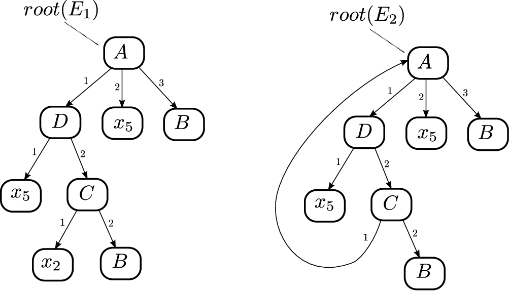
Refer to caption
Figure 1: Syntactic tree of E1=A⁡(D⁡(x5,C⁡(x2,B)),x5,B)E_{1}=A(D(x_{5},C(x_{2},B)),x_{5},B), and a graph presenting E2E_{2}

An example of a (standard finite) term is E1=A⁡(D⁡(x5,C⁡(x2,B)),x5,B)E_{1}=A(D(x_{5},C(x_{2},B)),x_{5},B) where the arities of A,B,C,DA,B,C,D are 3,0,2,23,0,2,2, respectively. The left-hand side of Fig. 1 depicts the syntactic tree of E1E_{1}. (The right-hand side E2E_{2} will be referred to later.)

Transitions are determined by a finite set of root-rewriting rules. An example of a “non-popping” rule is A⁡(x1,x2,x3)⟶aC⁡(D⁡(x3,B),x2)A(x_{1},x_{2},x_{3})\stackrel{{\scriptstyle a}}{{\longrightarrow}}C(D(x_{3},B),x_{2}), an example of a “popping” rule is A⁡(x1,x2,x3)⟶bx1A(x_{1},x_{2},x_{3})\stackrel{{\scriptstyle b}}{{\longrightarrow}}x_{1}. Each rule induces the transitions arising by applying the same substitution σ\sigma to both the left-hand side (lhs) and the right-hand side (rhs) of the rule. E.g., the rule

A⁡(x1,x2,x3)⟶aC⁡(D⁡(x3,B),x2)A(x_{1},x_{2},x_{3})\stackrel{{\scriptstyle a}}{{\longrightarrow}}C(D(x_{3},B),x_{2}) and the substitution σ\sigma for which σ⁡(x1)=D⁡(x5,C⁡(x2,B))\sigma(x_{1})=D(x_{5},C(x_{2},B)), σ⁡(x2)=x5\sigma(x_{2})=x_{5}, σ⁡(x3)=B\sigma(x_{3})=B

(where A⁡(x1,x2,x3)A(x_{1},x_{2},x_{3}) after applying σ\sigma becomes A⁡(D⁡(x5,C⁡(x2,B)),x5,B)A(D(x_{5},C(x_{2},B)),x_{5},B)) induce the transition A⁡(D⁡(x5,C⁡(x2,B)),x5,B)⟶aC⁡(D⁡(B,B),x5)A(D(x_{5},C(x_{2},B)),x_{5},B)\stackrel{{\scriptstyle a}}{{\longrightarrow}}C(D(B,B),x_{5}) depicted in Fig. 2.

Refer to caption
Figure 2: Transition generated by A⁡(x1,x2,x3)⟶aC⁡(D⁡(x3,B),x2)A(x_{1},x_{2},x_{3})\stackrel{{\scriptstyle a}}{{\longrightarrow}}C(D(x_{3},B),x_{2}) and σ\sigma (in the text)

Fig. 2 depicts an aa-transition between two states, where the states in our LTSs are terms. The small symbols x1,x2,x3x_{1},x_{2},x_{3} are superfluous here, they just depict the original variables in the lhs and in the rhs of the respective rule; these variables have been replaced by applying the substitution σ\sigma. Hence x3x_{3} and x2x_{2} in the target-term have been replaced by the third root-successor and by the second root-successor of the source-term, respectively. In this concrete case the first root-successor of the source-term “disappears” since x1x_{1} does not occur in the rhs of the rule.

Another example can be given by the rule A⁡(x1,x2,x3)⟶bx1A(x_{1},x_{2},x_{3})\stackrel{{\scriptstyle b}}{{\longrightarrow}}x_{1} and the above σ\sigma, which induces the transition, or the one-step path, F⟶bHF\stackrel{{\scriptstyle b}}{{\longrightarrow}}H where F=A⁡(D⁡(x5,C⁡(x2,B)),x5,B)F=A(D(x_{5},C(x_{2},B)),x_{5},B) and H=D⁡(x5,C⁡(x2,B))H=D(x_{5},C(x_{2},B)). In this case our one-step path exposes a root-successor HH in the source term FF (the first root-successor in our case); the path has thus “sinked” to a subterm in depth 11.

The result informally. We will show that there is an algorithm that computes EqLv​(T0,U0)\textsc{EqLv}(T_{0},U_{0}) when given a finite set of root-rewriting rules and two terms T0,U0T_{0},U_{0}. In the rest of this section we formalize this statement, making also some conventions about our use of (finite and infinite) terms and substitutions.

Regular terms, presentation size. We identify terms with their syntactic trees, and denote them by E,F,…E,F,\dots. Thus a term EE over 𝒩\mathcal{N} (where 𝒩\mathcal{N} is a set of ranked nonterminals) is a rooted, ordered, finite or infinite tree where each node has a label from 𝒩∪Var\mathcal{N}\cup\textsc{Var}; if the label of a node is xi∈Varx_{i}\in\textsc{Var}, then the node has no successors, and if the label is A∈𝒩A\in\mathcal{N}, then it has mm (immediate) successor-nodes where m=a​r​i​t​y​(A)m=arity(A). More precisely, a term corresponds to a set of isomorphic trees, since two isomorphic trees represent the same term. Each node is also the root of a subterm of EE, i.e., of the subtree rooted in this node; more precisely, each concrete node is the root of a subterm-occurrence, since a subterm corresponds to a set of isomorphic subtrees. A subterm can thus have more (maybe infinitely many) occurrences in EE. Each subterm-occurrence has its (nesting) depth in EE, which is its (naturally defined) distance from the root of EE; the term EE itself is a subterm-occurrence with depth 00. E.g., in E1=A⁡(D⁡(x5,C⁡(x2,B)),x5,B)E_{1}=A(D(x_{5},C(x_{2},B)),x_{5},B) (in Fig. 1) there is one occurrence of the term C⁡(x2,B)C(x_{2},B), with depth 22, and two occurrences of x5x_{5}, with depths 11 and 22.

We also use the standard notation: a term is either xix_{i} or A⁡(G1,…,Gm)A(G_{1},\dots,G_{m}); if E=A⁡(G1,…,Gm)E=A(G_{1},\dots,G_{m}), then root​(E)=A∈𝒩\textsc{root}(E)=A\in\mathcal{N}, m=a​r​i​t​y​(A)m=arity(A), and G1,…,GmG_{1},\dots,G_{m} are the root-successors, i.e., the ordered subterm-occurrences with depth 11.

A term EE is finite if the respective tree is finite; by 0​p​t​(E)0pt(E) we then mean the largest depth of a subterm-occurrence in EE. For E1=A⁡(D⁡(x5,C⁡(x2,B)),x5,B)E_{1}=A(D(x_{5},C(x_{2},B)),x_{5},B) in Fig. 1 we thus have 0​p​t​(E1)=30pt(E_{1})=3.

A (possibly infinite) term is regular if it has only finitely many subterms (though the subterms may be infinite and can have infinitely many occurrences). Any regular term has a natural finite-graph presentation (with possible cycles). E.g., the right-hand side of Fig. 1 presents a regular term E2E_{2}; here the term E2E_{2} itself is a subterm with infinitely many occurrences (with depths 0,3,6,…0,3,6,\dots). By PrSize​(E)\textsc{PrSize}(E) (the presentation size of EE) we mean the size of the smallest graph presentation of EE.

We can be more precise, though the respective notions are standard. A finite-graph presentation of a (regular) term over 𝒩\mathcal{N} is a finite directed (multi)graph, with a designated root, where each node has a label from 𝒩∪Var\mathcal{N}\cup\textsc{Var}; if the label of a node is xi∈Varx_{i}\in\textsc{Var}, then the node has no outgoing arcs, and if the label is A∈𝒩A\in\mathcal{N}, then the node has a​r​i​t​y​(A)arity(A) ordered outgoing arcs. The standard “tree-unfolding” of the graph is the respective term, which is infinite if there are cycles in the graph. We can obviously effectively compare if two graph presentations represent the same term. Given a presentation of a regular term EE, we can thus compute the syntactic graph of EE, i.e., the graph whose nodes (one-to-one) correspond to the (roots of) subterms occurring in EE. (E.g., the syntactic graph of E2E_{2} in Fig. 1 arises from the given graph presentation by merging the nodes with label x5x_{5} and merging those with label BB; but we note that if we replaced DD with CC, we could not merge the nodes with label CC.) We can take the number of nodes of the syntactic graph of EE as PrSize​(E)\textsc{PrSize}(E).

In what follows, by a “term” we mean a “regular term” if we do not say explicitly that the term is finite. (We do not consider non-regular terms.) We reserve symbols E,F,G,HE,F,G,H, and also T,U,V,WT,U,V,W, for denoting (regular) terms.

Substitutions, associative composition. By Terms𝒩\textsc{Terms}_{\mathcal{N}} we denote the set of all (regular) terms over a set 𝒩\mathcal{N} of (ranked) nonterminals. A substitution σ\sigma is a mapping

σ:Var→Terms𝒩\sigma:\textsc{Var}\rightarrow\textsc{Terms}_{\mathcal{N}} whose support supp​(σ)={xi∣σ⁡(xi)≠xi}\textsc{supp}(\sigma)=\{x_{i}\mid\sigma(x_{i})\neq x_{i}\}

is finite; we reserve the symbol σ\sigma for substitutions. By range​(σ)\textsc{range}(\sigma) we mean the set {σ⁡(xi)∣xi∈supp​(σ)}\{\sigma(x_{i})\mid x_{i}\in\textsc{supp}(\sigma)\}. By applying a substitution σ\sigma to a term EE we get the term E​σE\sigma that arises from EE by replacing each occurrence of xix_{i} with σ⁡(xi)\sigma(x_{i}). Hence E=xiE=x_{i} implies E​σ=xi​σ=σ⁡(xi)E\sigma=x_{i}\,\sigma=\sigma(x_{i}); we prefer the notation xi​σx_{i}\sigma to σ⁡(xi)\sigma(x_{i}).

The composition of substitutions, where σ=σ1​σ2\sigma=\sigma_{1}\sigma_{2} satisfies xi​σ=(xi​σ1)​σ2x_{i}\sigma=(x_{i}\sigma_{1})\sigma_{2}, can be easily verified to be associative. We thus write simply E​σ1​σ2E\sigma_{1}\sigma_{2} when meaning (E​σ1)​σ2(E\sigma_{1})\sigma_{2} or E⁡(σ1​σ2)E(\sigma_{1}\sigma_{2}).

First-order grammars. A first-order grammar, an FO-grammar or just a grammar for short, is a tuple 𝒢=(𝒩,Σ,ℛ)\mathcal{G}=(\mathcal{N},\Sigma,\mathcal{R}) where 𝒩\mathcal{N} is a finite set of ranked nonterminals, viewed as function symbols with arities, Σ\Sigma is a finite set of actions (or letters), and ℛ\mathcal{R} is a finite set of rules of the form

A⁡(x1,x2,…,xm)⟶aEA(x_{1},x_{2},\dots,x_{m})\stackrel{{\scriptstyle a}}{{\longrightarrow}}E

where A∈𝒩A\in\mathcal{N}, a​r​i​t​y​(A)=marity(A)=m, a∈Σa\in\Sigma, and EE is a finite term over 𝒩\mathcal{N} in which each occurring variable is from the set {x1,x2,…,xm}\{x_{1},x_{2},\dots,x_{m}\}.

Rule-based and action-based LTSs generated by grammars. Given 𝒢=(𝒩,Σ,ℛ)\mathcal{G}=(\mathcal{N},\Sigma,\mathcal{R}), by ℒ𝒢r=(Terms𝒩,ℛ,(⟶r)r∈ℛ)\mathcal{L}^{\textsc{r}}_{\mathcal{G}}=(\textsc{Terms}_{\mathcal{N}},\mathcal{R},(\stackrel{{\scriptstyle r}}{{\longrightarrow}})_{r\in\mathcal{R}}) we denote the (rule based) LTS where each rule rr of the form A⁡(x1,x2,…,xm)⟶aEA(x_{1},x_{2},\dots,x_{m})\stackrel{{\scriptstyle a}}{{\longrightarrow}}E induces (A⁡(x1,…,xm))​σ⟶rE​σ(A(x_{1},\dots,x_{m}))\sigma\stackrel{{\scriptstyle r}}{{\longrightarrow}}E\sigma for any substitution σ\sigma.
(Hence also A⁡(x1,…,xm)⟶rEA(x_{1},\dots,x_{m})\stackrel{{\scriptstyle r}}{{\longrightarrow}}E, due to σ\sigma with supp​(σ)=∅\textsc{supp}(\sigma)=\emptyset.)

Speaking in an informal “operational” manner, we can apply a rule rr of the form A⁡(x1,…,xm)⟶rEA(x_{1},\dots,x_{m})\stackrel{{\scriptstyle r}}{{\longrightarrow}}E to (a graph-presentation of) FF iff root​(F)=A\textsc{root}(F)=A. If so, and E=xjE=x_{j}, then the target of the jj-th outgoing arc of the root of FF (which might be the root itself in the case of a loop) is the root of HH where F⟶rHF\stackrel{{\scriptstyle r}}{{\longrightarrow}}H. If E∉VarE\not\in\textsc{Var}, we get HH (for which F⟶rHF\stackrel{{\scriptstyle r}}{{\longrightarrow}}H) by adding (a fresh copy of) EE to FF where the root of EE becomes the root of the arising HH; to finish the construction of HH, each arc in EE leading to a node labelled with xjx_{j} is redirected to the jj-th root-successor in FF. Hence the variables x1,…,xmx_{1},\dots,x_{m} in the rules serve just as “place-holders” for root-successors (in the source term of a transition); recall again Fig. 2.

The LTS ℒ𝒢r\mathcal{L}^{\textsc{r}}_{\mathcal{G}} is deterministic, since for each FF and rr there is at most one HH such that F⟶rHF\stackrel{{\scriptstyle r}}{{\longrightarrow}}H. Hence F⟶wF\stackrel{{\scriptstyle w}}{{\longrightarrow}}, for w∈ℛ∗w\in\mathcal{R}^{*}, refers to a unique path in ℒ𝒢r\mathcal{L}^{\textsc{r}}_{\mathcal{G}} (which is later technically convenient).

We stress explicitly that transitions cannot add variables, i.e., F⟶wHF\stackrel{{\scriptstyle w}}{{\longrightarrow}}H implies that each variable occurring in HH also occurs in FF (though not vice versa in general; recall that the first root-successor “disappeared” by the transition in Fig. 2, which also caused that the subterm x2x_{2} “disappeared”). We also note that F⟶wHF\stackrel{{\scriptstyle w}}{{\longrightarrow}}H implies F​σ⟶wH​σF\sigma\stackrel{{\scriptstyle w}}{{\longrightarrow}}H\sigma for any substitution σ\sigma; this follows from the fact that xix_{i} are dead, not enabling any action.
Finally we observe that our stipulation that the right-hand sides (rhs) EE in the grammar-rules A⁡(x1,…,xm)⟶aEA(x_{1},\dots,x_{m})\stackrel{{\scriptstyle a}}{{\longrightarrow}}E are finite implies that all terms reachable from a finite term are finite. (It turns out technically convenient to have the rhs finite while including regular terms into our LTSs.)

By the action-based LTS, related to a grammar 𝒢=(𝒩,Σ,ℛ)\mathcal{G}=(\mathcal{N},\Sigma,\mathcal{R}), we mean the LTS ℒ𝒢a=(Terms𝒩,Σ,(⟶a)a∈Σ)\mathcal{L}^{\textsc{a}}_{\mathcal{G}}=(\textsc{Terms}_{\mathcal{N}},\Sigma,(\stackrel{{\scriptstyle a}}{{\longrightarrow}})_{a\in\Sigma}) where each rule A⁡(x1,…,xm)⟶aEA(x_{1},\dots,x_{m})\stackrel{{\scriptstyle a}}{{\longrightarrow}}E induces

(A⁡(x1,…,xm))​σ⟶aE​σ(A(x_{1},\dots,x_{m}))\sigma\stackrel{{\scriptstyle a}}{{\longrightarrow}}E\sigma

for any substitution σ\sigma.

Hence F⟶wHF\stackrel{{\scriptstyle w}}{{\longrightarrow}}H in ℒ𝒢r\mathcal{L}^{\textsc{r}}_{\mathcal{G}} implies F⟶act​(w)HF\stackrel{{\scriptstyle\textsc{act}(w)}}{{\longrightarrow}}H in ℒ𝒢a\mathcal{L}^{\textsc{a}}_{\mathcal{G}}, where act​(w)\textsc{act}(w) is the naturally defined action-image of ww: the homomorphism act:ℛ∗→Σ∗\textsc{act}:\mathcal{R}^{*}\rightarrow\Sigma^{*} is defined by putting act​(r)=a\textsc{act}(r)=a for any rule rr of the form A⁡(x1,…,xm)⟶aEA(x_{1},\dots,x_{m})\stackrel{{\scriptstyle a}}{{\longrightarrow}}E.

We note that ℒ𝒢a\mathcal{L}^{\textsc{a}}_{\mathcal{G}} is image-finite, and nondeterministic in general. In fact, we still complete the definition of ℒ𝒢a\mathcal{L}^{\textsc{a}}_{\mathcal{G}} by stipulating that

no ℬ⊆Terms𝒩×Terms𝒩\mathcal{B}\subseteq\textsc{Terms}_{\mathcal{N}}\times\textsc{Terms}_{\mathcal{N}} covers (xi,H)(x_{i},H) or (H,xi)(H,x_{i}) when H≠xiH\neq x_{i}.

We thus have that

xi≠Hx_{i}\neq H implies xi≁1Hx_{i}\not\sim_{1}H, i.e., EqLv​(xi,H)=0\textsc{EqLv}(x_{i},H)=0.

In particular we have xi≁1xjx_{i}\not\sim_{1}x_{j} for i≠ji\neq j. Technically we think of each used variable x∈Varx\in\textsc{Var} as being equipped with its unique action axa_{x} and with the transition x⟶axxx\stackrel{{\scriptstyle a_{x}}}{{\longrightarrow}}x in ℒ𝒢a\mathcal{L}^{\textsc{a}}_{\mathcal{G}}; this entails that xi≁1Hx_{i}\not\sim_{1}H for H≠xiH\neq x_{i} without any special stipulation.

Convention. Whenever we consider F⟶wHF\stackrel{{\scriptstyle w}}{{\longrightarrow}}H in ℒ𝒢a\mathcal{L}^{\textsc{a}}_{\mathcal{G}}, we tacitly assume that no special transitions x⟶axxx\stackrel{{\scriptstyle a_{x}}}{{\longrightarrow}}x are involved. Hence F⟶wHF\stackrel{{\scriptstyle w}}{{\longrightarrow}}H implies F​σ⟶wH​σF\sigma\stackrel{{\scriptstyle w}}{{\longrightarrow}}H\sigma for any substitution σ\sigma. We also stipulate that ∅\emptyset covers (xi,xi)(x_{i},x_{i}), thus avoiding superfluous technicalities.

The stipulation xi≁1Hx_{i}\not\sim_{1}H for H≠xiH\neq x_{i} reflects the fact that xi≠Hx_{i}\neq H implies that xiσ≁1Hσx_{i}\sigma\not\sim_{1}H\sigma for some σ\sigma, unless the underlying grammar 𝒢\mathcal{G} is trivial. The special transitions x⟶axxx\stackrel{{\scriptstyle a_{x}}}{{\longrightarrow}}x are just one technical possibility how to reflect this fact in ℒ𝒢a\mathcal{L}^{\textsc{a}}_{\mathcal{G}} smoothly.

In what follows we refer to the action-based LTSs ℒ𝒢a\mathcal{L}^{\textsc{a}}_{\mathcal{G}}, if we do not say explicitly that we have ℒ𝒢r\mathcal{L}^{\textsc{r}}_{\mathcal{G}} in mind.

Theorem 2.1

There is an algorithm that, given an FO-grammar 𝒢=(𝒩,Σ,ℛ)\mathcal{G}=(\mathcal{N},\Sigma,\mathcal{R}) and T0,U0∈Terms​(𝒩)T_{0},U_{0}\in\textsc{Terms}(\mathcal{N}), computes EqLv​(T0,U0)\textsc{EqLv}(T_{0},U_{0}) in ℒ𝒢a\mathcal{L}^{\textsc{a}}_{\mathcal{G}}.

3 Proof of Theorem 2.1

We note that deciding ∼0\sim_{0} is trivial, since T∼0UT\sim_{0}U holds for all T,UT,U. When having a procedure deciding ∼k\sim_{k}, we can easily construct a procedure deciding ∼k+1\sim_{k+1}; this follows from the facts that T∼k+1UT\sim_{k+1}U iff (T,U)(T,U) is covered by ∼k\sim_{k}, and that for any VV we can construct all (finitely many) pairs (a,V′)(a,V^{\prime}) such that V⟶aV′V\stackrel{{\scriptstyle a}}{{\longrightarrow}}V^{\prime}. We thus get a part of Theorem 2.1:

Proposition 1

There is an algorithm that, given 𝒢\mathcal{G} and T0,U0T_{0},U_{0}, outputs EqLv​(T0,U0)\textsc{EqLv}(T_{0},U_{0}) if T0≁U0T_{0}\not\sim U_{0}, and does not halt if T0∼U0T_{0}\sim U_{0}.

We need to modify the algorithm so that it recognizes the case T0∼U0T_{0}\sim U_{0} in finite time. As a convenient tool we introduce a round-based game between Prover(she) and Refuter(he); the game is more involved than the standard bisimulation game. We start with a simple first version of the game, and then we enhance it stepwise. Refuter will be always able to force his win in finite time if the terms in the initial pair (T0,U0)(T_{0},U_{0}) are non-equivalent. Prover will be always able to avoid losing if T0∼U0T_{0}\sim U_{0}, but only in the last game-version she will be able to force her win in finite time. Since Prover’s winning strategy for T0∼U0T_{0}\sim U_{0} in the last game-version will be finitely presentable and effectively verifiable, a proof of Theorem 2.1 will be finished. Before the first game-version we observe some simple standard facts related to (stratified) bisimulation equivalence.

Expansions. Assume an LTS ℒ=(𝒮,Σ,(⟶a)a∈Σ)\mathcal{L}=(\mathcal{S},\Sigma,(\stackrel{{\scriptstyle a}}{{\longrightarrow}})_{a\in\Sigma}). By

ℬ⊲ℬ′\mathcal{B}\lhd\mathcal{B}^{\prime}, where ℬ,ℬ′⊆𝒮×𝒮\mathcal{B},\mathcal{B}^{\prime}\subseteq\mathcal{S}\times\mathcal{S},

we denote that ℬ′\mathcal{B}^{\prime} is a minimal expansion for ℬ\mathcal{B}, i.e., ℬ′\mathcal{B}^{\prime} covers ℬ\mathcal{B} and no proper subset of ℬ′\mathcal{B}^{\prime} covers ℬ\mathcal{B}; this also implies that for each (s′,t′)∈ℬ′(s^{\prime},t^{\prime})\in\mathcal{B}^{\prime} there is (s,t)∈ℬ(s,t)\in\mathcal{B} such that s⟶as′s\stackrel{{\scriptstyle a}}{{\longrightarrow}}s^{\prime} and t⟶at′t\stackrel{{\scriptstyle a}}{{\longrightarrow}}t^{\prime} for some a∈Σa\in\Sigma. We note that ∅⊲∅\emptyset\lhd\emptyset, and if s,ts,t are dead (not enabling any action), then {(s,t)}⊲∅\{(s,t)\}\lhd\emptyset.

For any k∈ℕk\in\mathbb{N} we have k<ωk<\omega and we stipulate ω−k=ω+k=ω\omega-k=\omega+k=\omega. We also stipulate min⁡∅=ω\min\emptyset=\omega, and define MinEqL​(ℬ)=min⁡{EqLv​(s,t)∣(s,t)∈ℬ}\textsc{MinEqL}(\mathcal{B})=\min\{\textsc{EqLv}(s,t)\mid(s,t)\in\mathcal{B}\}.

Proposition 2

(1) If MinEqL​(ℬ)=0\textsc{MinEqL}(\mathcal{B})=0 then there is no ℬ′\mathcal{B}^{\prime} such that ℬ⊲ℬ′\mathcal{B}\lhd\mathcal{B}^{\prime}.
(2) If ℬ⊲ℬ′\mathcal{B}\lhd\mathcal{B}^{\prime} and MinEqL​(ℬ)<ω\textsc{MinEqL}(\mathcal{B})<\omega, then MinEqL​(ℬ)>MinEqL​(ℬ′)\textsc{MinEqL}(\mathcal{B})>\textsc{MinEqL}(\mathcal{B}^{\prime}).
(3) If MinEqL​(ℬ)>0\textsc{MinEqL}(\mathcal{B})>0 then there is ℬ′\mathcal{B}^{\prime} such that ℬ⊲ℬ′\mathcal{B}\lhd\mathcal{B}^{\prime} and MinEqL​(ℬ′)≥MinEqL​(ℬ)−1\textsc{MinEqL}(\mathcal{B}^{\prime})\geq\textsc{MinEqL}(\mathcal{B})-1. (In particular, if ℬ⊆∼\mathcal{B}\subseteq\,\sim then ℬ⊲ℬ′\mathcal{B}\lhd\mathcal{B}^{\prime} for some ℬ′⊆∼\mathcal{B}^{\prime}\subseteq\,\sim.)
(4) For k∈ℕk\in\mathbb{N} we have s∼kts\sim_{k}t iff there is a sequence {(s,t)}⊲ℬ1⊲ℬ2⊲⋯⊲ℬk\{(s,t)\}\lhd\mathcal{B}_{1}\lhd\mathcal{B}_{2}\lhd\cdots\lhd\mathcal{B}_{k}.

Prover-Refuter game (first version). A play starts with a grammar 𝒢=(𝒩,Σ,ℛ)\mathcal{G}=(\mathcal{N},\Sigma,\mathcal{R}) and an initial pair (T0,U0)(T_{0},U_{0}) of terms. For i=0,1,2​…i=0,1,2\dots, the (i+1)(i{+}1)-th round of the play starts with some specified pair (Ti,Ui)(T_{i},U_{i}) and proceeds as follows:

  1. 1.

    Prover chooses k>0k>0 and some ℬj⊆Terms𝒩×Terms𝒩\mathcal{B}_{j}\subseteq\textsc{Terms}_{\mathcal{N}}\times\textsc{Terms}_{\mathcal{N}} for j=1,2​…,kj=1,2\dots,k and shows that ℬ0⊲ℬ1⊲ℬ2⊲…⊲ℬk\mathcal{B}_{0}\lhd\mathcal{B}_{1}\lhd\mathcal{B}_{2}\lhd\ldots\lhd\mathcal{B}_{k} where ℬ0={(Ti,Ui)}\mathcal{B}_{0}=\{(T_{i},U_{i})\}.
    If this is impossible (i.e., if Ti≁1UiT_{i}\not\sim_{1}U_{i}), then Refuter wins.

  2. 2.

    Refuter chooses a pair (Ti′,Ui′)(T^{\prime}_{i},U^{\prime}_{i}) in ℬk∖⋃j=0k−1ℬj\mathcal{B}_{k}\smallsetminus\bigcup_{j=0}^{k-1}\mathcal{B}_{j}. If this is impossible, i.e. if ℬk⊆⋃j=0k−1ℬj\mathcal{B}_{k}\subseteq\bigcup_{j=0}^{k-1}\mathcal{B}_{j} (which includes the case ℬk=∅\mathcal{B}_{k}=\emptyset), then Prover wins. (In this case Ti∼UiT_{i}\sim U_{i}, since Ti≁UiT_{i}\not\sim U_{i} implies that ℬk⊈⋃j=0k−1ℬj\mathcal{B}_{k}\not\subseteq\bigcup_{j=0}^{k-1}\mathcal{B}_{j}, by Prop. 2(2).)

  3. 3.

    The pair (Ti+1,Ui+1)=(Ti′,Ui′)(T_{i+1},U_{i+1})=(T^{\prime}_{i},U^{\prime}_{i}) is taken for starting the (i+2)(i{+}2)-th round.

Refer to caption
Figure 3: Illustration of a game-round (where Prover has chosen k=5k=5)

Fig. 3 illustrates an (i+1)(i{+}1)-th round (with k=5k{=}5). Note that our requirement ℬ0⊲ℬ1⊲⋯⊲ℬk\mathcal{B}_{0}\lhd\mathcal{B}_{1}\lhd\cdots\lhd\mathcal{B}_{k} entails that there are u1,u2∈ℛ∗u_{1},u_{2}\in\mathcal{R}^{*} such that |u1|=|u2|=k|u_{1}|=|u_{2}|=k, act​(u1)=act​(u2)\textsc{act}(u_{1})=\textsc{act}(u_{2}), and Ti⟶u1Ti′T_{i}\stackrel{{\scriptstyle u_{1}}}{{\longrightarrow}}T^{\prime}_{i}, Ui⟶u2Ui′U_{i}\stackrel{{\scriptstyle u_{2}}}{{\longrightarrow}}U^{\prime}_{i} (in ℒ𝒢r\mathcal{L}^{\textsc{r}}_{\mathcal{G}}), as sketched in the figure.

The reversals of u1,u2u_{1},u_{2} can be found by the “bottom-up approach”, starting from (Ti′,Ui′)(T^{\prime}_{i},U^{\prime}_{i}) and going up to (Ti,Ui)(T_{i},U_{i}). This follows from recalling that ℬ⊲ℬ′\mathcal{B}\lhd\mathcal{B}^{\prime} implies that for each (G′,H′)∈ℬ′(G^{\prime},H^{\prime})\in\mathcal{B}^{\prime} there is (G,H)∈ℬ(G,H)\in\mathcal{B} such that G⟶aG′G\stackrel{{\scriptstyle a}}{{\longrightarrow}}G^{\prime} and H⟶aH′H\stackrel{{\scriptstyle a}}{{\longrightarrow}}H^{\prime} for some a∈Σa\in\Sigma.

We also note that, e.g., for each VV such that Ti⟶vVT_{i}\stackrel{{\scriptstyle v}}{{\longrightarrow}}V in ℒ𝒢r\mathcal{L}^{\textsc{r}}_{\mathcal{G}} where |v|=j≤k|v|=j\leq k there is v′∈ℛ∗v^{\prime}\in\mathcal{R}^{*} and V′V^{\prime} such that |v′|=|v||v^{\prime}|=|v|, act​(v)=act​(v′)\textsc{act}(v)=\textsc{act}(v^{\prime}), Ui⟶v′V′U_{i}\stackrel{{\scriptstyle v^{\prime}}}{{\longrightarrow}}V^{\prime}, and (V,V′)∈ℬj(V,V^{\prime})\in\mathcal{B}_{j}.

This is also depicted in Fig. 3. When looking for Ui⟶v′V′U_{i}\stackrel{{\scriptstyle v^{\prime}}}{{\longrightarrow}}V^{\prime}, we now use the “top-down approach” driven by Ti⟶vVT_{i}\stackrel{{\scriptstyle v}}{{\longrightarrow}}V.

We say that Refuter uses the least-eqlevel strategy, if he always chooses (Ti′,Ui′)(T^{\prime}_{i},U^{\prime}_{i}) so that EqLv​(Ti′,Ui′)=MinEqL​(ℬk)\textsc{EqLv}(T^{\prime}_{i},U^{\prime}_{i})=\textsc{MinEqL}(\mathcal{B}_{k}); in this case EqLv​(Ti′,Ui′)<MinEqL​(⋃j=0k−1ℬj)\textsc{EqLv}(T^{\prime}_{i},U^{\prime}_{i})<\textsc{MinEqL}(\bigcup_{j=0}^{k-1}\mathcal{B}_{j}), and thus EqLv​(Ti′,Ui′)<EqLv​(Ti,Ui)−(k−1)\textsc{EqLv}(T^{\prime}_{i},U^{\prime}_{i})<\textsc{EqLv}(T_{i},U_{i})-(k{-}1), unless T∼UT\sim U for all (T,U)∈⋃j=0kℬj(T,U)\in\bigcup_{j=0}^{k}\mathcal{B}_{j}. We easily observe the following facts.

Proposition 3

Let EqLv​(T0,U0)=e∈ℕ∪{ω}\textsc{EqLv}(T_{0},U_{0})=e\in\mathbb{N}\cup\{\omega\}.
1. If e<ωe<\omega, then Refuter wins within e+1e{+}1 rounds by the least-eqlevel strategy.
2. Prover can guarantee that she will not lose within ee rounds.

Prover’s additional tool. A challenge is to add sound possibilities for Prover to enable her to force her win in finite time if T0∼U0T_{0}\sim U_{0}. We allow Prover to claim a win when she can (soundly) demonstrate, in some (i+1)(i{+}1)-th round, that either Refuter has not used the least-eqlevel strategy or T0∼U0T_{0}\sim U_{0}. This new abstract rule does not change Prop. 3. A simple instance is a repeat: if {Ti,Ui}={Tj,Uj}\{T_{i},U_{i}\}=\{T_{j},U_{j}\} for some j<ij<i, then Prover can claim her win. (Equality Ti=UiT_{i}=U_{i} is another trivial example.)

We thus further assume that Prover wins when a repeat appears, and we look at more involved options enabling her to “balance”, i.e., to replace Ti′,Ui′T^{\prime}_{i},U^{\prime}_{i} (in the point 33 of a game-round) with Ti+1,Ui+1T_{i+1},U_{i+1} that are “closer” to each other, while keeping EqLv​(Ti+1,Ui+1)=EqLv​(Ti′,Ui′)\textsc{EqLv}(T_{i+1},U_{i+1})=\textsc{EqLv}(T^{\prime}_{i},U^{\prime}_{i}) when Refuter uses the least eq-level strategy. Before formulating the second version of the game, we clarify the crucial underlying facts. First a trivial one:

Proposition 4

Assume an LTS ℒ\mathcal{L}. If EqLv​(s,t)=k\textsc{EqLv}(s,t){=}k and EqLv​(s,s′)>k\textsc{EqLv}(s,s^{\prime})>k, then EqLv​(s′,t)=k\textsc{EqLv}(s^{\prime},t)=k (since s′∼ks∼kts^{\prime}\sim_{k}s\sim_{k}t and s′∼k+1s≁k+1ts^{\prime}\sim_{k+1}s\not\sim_{k+1}t).

Congruence, the crux of balancing. We assume a given grammar 𝒢=(𝒩,Σ,ℛ)\mathcal{G}=(\mathcal{N},\Sigma,\mathcal{R}). For substitutions σ,σ′\sigma,\sigma^{\prime} and k∈ℕ∪{ω}k\in\mathbb{N}\cup\{\omega\} we put

σ∼kσ′\sigma\sim_{k}\sigma^{\prime} if xiσ∼kxiσ′x_{i}\sigma\sim_{k}x_{i}\sigma^{\prime} for each xi∈Varx_{i}\in\textsc{Var}.

We also put EqLv(σ,σ′)=max{k∈ℕ∪{ω}∣σ∼kσ′}\textsc{EqLv}(\sigma,\sigma^{\prime})=\max\,\{\,k\in\mathbb{N}\cup\{\omega\}\mid\sigma\sim_{k}\sigma^{\prime}\}; hence EqLv​(σ,σ′)=min⁡{EqLv​(xi​σ,xi​σ′)∣xi∈Var}\textsc{EqLv}(\sigma,\sigma^{\prime})=\min\,\{\,\textsc{EqLv}(x_{i}\sigma,x_{i}\sigma^{\prime})\mid x_{i}\in\textsc{Var}\}. We now note that ∼k\sim_{k} and ∼=∼ω\sim=\sim_{\omega} are congruences:

Proposition 5

(1) If E∼kFE\sim_{k}F, then Eσ∼kFσE\sigma\sim_{k}F\sigma; hence EqLv​(E,F)≤EqLv​(E​σ,F​σ)\textsc{EqLv}(E,F)\leq\textsc{EqLv}(E\sigma,F\sigma).
(2) If σ∼kσ′\sigma\sim_{k}\sigma^{\prime}, then Eσ∼kEσ′E\sigma\sim_{k}E\sigma^{\prime}; hence EqLv​(σ,σ′)≤EqLv​(E​σ,E​σ′)\textsc{EqLv}(\sigma,\sigma^{\prime})\leq\textsc{EqLv}(E\sigma,E\sigma^{\prime}).
Moreover, if σ∼kσ′\sigma\sim_{k}\sigma^{\prime} and E∉VarE\not\in\textsc{Var} (i.e., root​(E)∈𝒩\textsc{root}(E)\in\mathcal{N}), then Eσ∼k+1Eσ′E\sigma\sim_{k+1}E\sigma^{\prime}.

Proof

(1) Suppose {(E,F)}=ℬ0⊲ℬ1⊲ℬ2⊲⋯⊲ℬk\{(E,F)\}=\mathcal{B}_{0}\lhd{\mathcal{B}_{1}}\lhd{\mathcal{B}_{2}}\cdots\lhd{\mathcal{B}_{k}}; note that any pair (xi,H)(x_{i},H), or (H,xi)(H,x_{i}), in ⋃j=0k−1ℬj\bigcup_{j=0}^{k-1}\mathcal{B}_{j} must satisfy H=xiH=x_{i} (since otherwise it cannot be covered by our definition of ℒ𝒢a\mathcal{L}^{\textsc{a}}_{\mathcal{G}}). For each j∈[0,k]j\in[0,k] we put ℬj′={(G​σ,H​σ)∣(G,H)∈ℬj}\mathcal{B}^{\prime}_{j}=\{(G\sigma,H\sigma)\mid(G,H)\in\mathcal{B}_{j}\}. We almost get {(E​σ,F​σ)}=ℬ0′⊲ℬ1′⊲ℬ2′⊲⋯⊲ℬk′\{(E\sigma,F\sigma)\}=\mathcal{B}^{\prime}_{0}\lhd{\mathcal{B}^{\prime}_{1}}\lhd{\mathcal{B}^{\prime}_{2}}\lhd\cdots\lhd{\mathcal{B}^{\prime}_{k}}; just for the cases (xi,xi)∈ℬj(x_{i},x_{i})\in\mathcal{B}_{j}, j∈[0,k−1]j\in[0,k{-}1], where (xi​σ,xi​σ)(x_{i}\sigma,x_{i}\sigma) is not covered by ℬj+1′\mathcal{B}^{\prime}_{j+1}, we complete ℬj+1′,ℬj+2′,…,ℬk′\mathcal{B}^{\prime}_{j+1},\mathcal{B}^{\prime}_{j+2},\dots,\mathcal{B}^{\prime}_{k} with some pairs of identical terms, using the fact that {(E,E)}⊲{(E′,E′)∣E⟶aE′\{(E,E)\}\lhd\{(E^{\prime},E^{\prime})\mid E\stackrel{{\scriptstyle a}}{{\longrightarrow}}E^{\prime} for some a∈Σ}a\in\Sigma\}).

(2) Suppose σ∼kσ′\sigma\sim_{k}\sigma^{\prime}, and take {(E,E)}=ℬ0⊲ℬ1⊲ℬ2⊲⋯⊲ℬk\{(E,E)\}=\mathcal{B}_{0}\lhd{\mathcal{B}_{1}}\lhd{\mathcal{B}_{2}}\cdots\lhd{\mathcal{B}_{k}} where ⋃j=0kℬj⊆{(F,F)∣F∈Terms𝒩}\bigcup_{j=0}^{k}\mathcal{B}_{j}\subseteq\,\{(F,F)\mid F\in\textsc{Terms}_{\mathcal{N}}\}. Let ℬj′={(G​σ,G​σ′)∣(G,G)∈ℬj}\mathcal{B}^{\prime}_{j}=\{(G\sigma,G\sigma^{\prime})\mid(G,G)\in\mathcal{B}_{j}\}. For the cases (xi,xi)∈ℬj(x_{i},x_{i})\in\mathcal{B}_{j}, and thus (xi​σ,xi​σ′)∈ℬj′(x_{i}\sigma,x_{i}\sigma^{\prime})\in\mathcal{B}^{\prime}_{j}, we complete ℬj+1′,ℬj+2′,…​ℬk′\mathcal{B}^{\prime}_{j+1},\mathcal{B}^{\prime}_{j+2},\dots\mathcal{B}^{\prime}_{k} accordingly, using the fact that xiσ∼kxiσ′x_{i}\sigma\sim_{k}x_{i}\sigma^{\prime}. If E∉VarE\not\in\textsc{Var}, then this procedure is valid even when we start with {(E,E)}=ℬ0⊲ℬ1⊲ℬ2⊲⋯⊲ℬk+1\{(E,E)\}=\mathcal{B}_{0}\lhd{\mathcal{B}_{1}}\lhd{\mathcal{B}_{2}}\cdots\lhd{\mathcal{B}_{k+1}}. ∎

Remark. The compositionality induced by the congruence properties leads naturally to considering the following modification of our game, based on decompositions. Prover is always allowed to “decompose” (Ti,Ui)(T_{i},U_{i}), i.e., to present some finite set ℬ\mathcal{B} of pairs of terms that are in some sense smaller than (Ti,Ui)(T_{i},U_{i}), if it is guaranteed that EqLv​(Ti,Ui)≥MinEqL​(ℬ)\textsc{EqLv}(T_{i},U_{i})\geq\textsc{MinEqL}(\mathcal{B}); Refuter then chooses a pair from ℬ\mathcal{B} for continuing. If our measure of size satisfies that there are only finitely many pairs with the size that is smaller than or equal to the size of any given (T,U)(T,U), then Refuter’s least-eqlevel strategy still wins if the initial terms are non-equivalent. On the other hand, if there is a bound such that each pair T∼UT\sim U that is bigger than the bound is decomposable via a set ℬ⊆∼\mathcal{B}\subseteq\sim, then we have a required algorithm: if Prover keeps decomposing large pairs via subsets of ∼\sim, then we get a repeat eventually.

This is a basis of decision algorithms for so called BPA processes, which can be viewed as being generated by FO-grammars where all nonterminals have arity 11 (or 00). We can refer, e.g., to the papers [4, 3, 11] for details. However, in our more general case such a straightforward approach does not seem clear. We follow a more involved way, based on a balancing strategy that makes the component-terms in (Ti,Ui)(T_{i},U_{i}) “close to each other”. We note that balancing strategies, in different frameworks, were used by Sénizergues [15, 16, 17] and then Stirling [19, 20, 21]. In fact, we will also discuss a bit of decomposition later, in Section 4.

We now illustrate how Prover can use already the simple fact captured by Prop. 4. Suppose the (i+1)(i{+}1)-th round starts with (Ti,Ui)(T_{i},U_{i}) and Refuter chooses (Ti′,Ui′)(T^{\prime}_{i},U^{\prime}_{i}) in ℬk\mathcal{B}_{k} (we refer to the notation in the game definition, and to Fig. 3). We thus have Ti⟶u1Ti′T_{i}\stackrel{{\scriptstyle u_{1}}}{{\longrightarrow}}T^{\prime}_{i}, Ui⟶u2Ui′U_{i}\stackrel{{\scriptstyle u_{2}}}{{\longrightarrow}}U^{\prime}_{i} in ℒ𝒢r\mathcal{L}^{\textsc{r}}_{\mathcal{G}}, for some u1,u2∈ℛ∗u_{1},u_{2}\in\mathcal{R}^{*}, where |u1|=|u2|=k|u_{1}|=|u_{2}|=k (and act​(u1)=act​(u2)\textsc{act}(u_{1})=\textsc{act}(u_{2})).

Suppose that Ti⟶u1Ti′T_{i}\stackrel{{\scriptstyle u_{1}}}{{\longrightarrow}}T^{\prime}_{i} is not a shortest path from TiT_{i} to Ti′T^{\prime}_{i} (in ℒ𝒢r\mathcal{L}^{\textsc{r}}_{\mathcal{G}}); then we have Ti⟶v1Ti′T_{i}\stackrel{{\scriptstyle v_{1}}}{{\longrightarrow}}T^{\prime}_{i} for some v1∈ℛ∗v_{1}\in\mathcal{R}^{*} where |v1|<|u1||v_{1}|<|u_{1}|. As we already observed, we then must also have Ui⟶v2U′′U_{i}\stackrel{{\scriptstyle v_{2}}}{{\longrightarrow}}U^{\prime\prime} for some U′′U^{\prime\prime} and some v2∈ℛ∗v_{2}\in\mathcal{R}^{*} such that |v1|=|v2||v_{1}|=|v_{2}| and (Ti′,U′′)∈⋃j=0k−1ℬj(T^{\prime}_{i},U^{\prime\prime})\in\bigcup_{j=0}^{k-1}\mathcal{B}_{j}. (In Fig. 3 we would have a respective pair (V,V′)=(Ti′,U′′)(V,V^{\prime})=(T^{\prime}_{i},U^{\prime\prime}).) We thus have EqLv​(Ti′,U′′)>EqLv​(Ti′,Ui′)\textsc{EqLv}(T^{\prime}_{i},U^{\prime\prime})>\textsc{EqLv}(T^{\prime}_{i},U^{\prime}_{i}) when Ti′≁Ui′T^{\prime}_{i}\not\sim U^{\prime}_{i} and Refuter uses the least-eqlevel strategy.

Therefore Refuter “cannot protest” when Prover puts (Ti+1,Ui+1)=(U′′,Ui′)(T_{i+1},U_{i+1})=(U^{\prime\prime},U^{\prime}_{i}) instead of (Ti+1,Ui+1)=(Ti′,Ui′)(T_{i+1},U_{i+1})=(T^{\prime}_{i},U^{\prime}_{i}), since EqLv​(Ti′,Ui′)=EqLv​(U′′,Ui′)\textsc{EqLv}(T^{\prime}_{i},U^{\prime}_{i})=\textsc{EqLv}(U^{\prime\prime},U^{\prime}_{i}) if Refuter uses the least-eqlevel strategy. We note that U′′,Ui′U^{\prime\prime},U^{\prime}_{i} are close to each other in the sense that they are both reachable within kk steps from one “pivot term”, namely UiU_{i}. We have Ui↝k(U′′,Ui′)U_{i}\leadsto_{k}(U^{\prime\prime},U^{\prime}_{i}), where generally we define

W↝kT⇔dfW⟶vTW\leadsto_{k}T\Leftrightarrow_{\text{df}}W\stackrel{{\scriptstyle v}}{{\longrightarrow}}T for some v​ of length at most ​kv\text{ of length at most }k, and W↝k(T,U)⇔dfW↝kTW\leadsto_{k}(T,U)\Leftrightarrow_{\text{df}}W\leadsto_{k}T and W↝kUW\leadsto_{k}U. (1)

In the second game-version below we use the congruence properties to enable Prover to replace (Ti′,Ui′)(T^{\prime}_{i},U^{\prime}_{i}) with “closer” (Ti+1,Ui+1)(T_{i+1},U_{i+1}) even in some cases where Ti⟶u1Ti′T_{i}\stackrel{{\scriptstyle u_{1}}}{{\longrightarrow}}T^{\prime}_{i} is a shortest path from TiT_{i} to Ti′T^{\prime}_{i} and Ui⟶u2Ui′U_{i}\stackrel{{\scriptstyle u_{2}}}{{\longrightarrow}}U^{\prime}_{i} is a shortest path from UiU_{i} to Ui′U^{\prime}_{i}.

Prover-Refuter game (second version). The only change w.r.t. the first game-version is in the point 33:

  1. 3.

    Prover creates (Ti+1,Ui+1)(T_{i+1},U_{i+1}) for the start of the (i+2)(i{+}2)-th round:

    Either she puts (Ti+1,Ui+1)=(Ti′,Ui′)(T_{i+1},U_{i+1})=(T^{\prime}_{i},U^{\prime}_{i}), thus making no change, or she can use one of the following options if available:

    1. i/

      Left-balancing: Prover presents Ti′T^{\prime}_{i} as G​σG\sigma for some finite term GG and some substitution σ\sigma, where for each V∈range​(σ)V\in\textsc{range}(\sigma) she finds V′V^{\prime} such that (V,V′)∈⋃j=0k−1ℬj(V,V^{\prime})\in\bigcup_{j=0}^{k-1}\mathcal{B}_{j}. She defines σ′\sigma^{\prime} with supp​(σ′)=supp​(σ)\textsc{supp}(\sigma^{\prime})=\textsc{supp}(\sigma) as follows: if σ⁡(xℓ)=V\sigma(x_{\ell})=V, then σ′​(xℓ)=V′\sigma^{\prime}(x_{\ell})=V^{\prime}, where (V,V′)(V,V^{\prime}) is an above found pair. Finally she puts (Ti+1,Ui+1)=(G​σ′,Ui′)(T_{i+1},U_{i+1})=(G\sigma^{\prime},U^{\prime}_{i}).

    2. ii/

      Right-balancing: Symmetrically, Prover presents Ui′U^{\prime}_{i} as G​σG\sigma, finds all appropriate pairs (V′,V)(V^{\prime},V) in ⋃j=0k−1ℬj\bigcup_{j=0}^{k-1}\mathcal{B}_{j}, and puts (Ti+1,Ui+1)=(Ti′,G​σ′)(T_{i+1},U_{i+1})=(T^{\prime}_{i},G\sigma^{\prime}).

Our previous illustration, where Ti⟶uiTi′T_{i}\stackrel{{\scriptstyle u_{i}}}{{\longrightarrow}}T^{\prime}_{i} was not a shortest path from TiT_{i} to Ti′T^{\prime}_{i}, was a special case: we had Ti′=G​σT^{\prime}_{i}=G\sigma where G=x1G=x_{1}, supp​(σ)={x1}\textsc{supp}(\sigma)=\{x_{1}\} and x1​σ=Ti′x_{1}\sigma=T^{\prime}_{i}, and we replaced G​σG\sigma with G​σ′G\sigma^{\prime} where x1​σ′=U′′x_{1}\sigma^{\prime}=U^{\prime\prime} (and thus (xi​σ,xi​σ′)∈⋃j=0k−1ℬj(x_{i}\sigma,x_{i}\sigma^{\prime})\in\bigcup_{j=0}^{k-1}\mathcal{B}_{j} for all xi∈supp​(σ)=supp​(σ′)={x1}x_{i}\in\textsc{supp}(\sigma)=\textsc{supp}(\sigma^{\prime})=\{x_{1}\}).

Informally speaking, in the second game-version Prover might replace the whole Ti′T^{\prime}_{i} with some U′′U^{\prime\prime} that is “shortly reachable from the pivot” (if possible), but she can also replace just “small-depth” subterms VV of Ti′T^{\prime}_{i} with (sub)terms V′V^{\prime} that are “shortly reachable from the pivot”; in the latter case some “special finite head” GG of Ti′T^{\prime}_{i} remains. (The case of right-balancings is symmetric.)

A left-balancing (with the pivot W=UiW=U_{i} and the bal-result (G​σ′,Ui′)(G\sigma^{\prime},U^{\prime}_{i})) is also depicted in the upper part of Fig. 4. (The lower part will be discussed later.)

Refer to caption
Figure 4: Two consecutive rounds, with a left-balancing in the first one

We can easily verify that Prop. 3 holds also for the second game-version. The crucial point is that EqLv​(Ti+1,Ui+1)=EqLv​(Ti′,Ui′)\textsc{EqLv}(T_{i+1},U_{i+1})=\textsc{EqLv}(T^{\prime}_{i},U^{\prime}_{i}) when Refuter uses the least-eqlevel strategy (this is based on Prop. 5(2) and Prop. 4).

Bal-results are close to pivots. When doing a left-balancing, replacing (Ti′,Ui′)=(G​σ,Ui′)(T^{\prime}_{i},U^{\prime}_{i})=(G\sigma,U^{\prime}_{i}) with the bal-result (Ti+1,Ui+1)=(G​σ′,Ui′)(T_{i+1},U_{i+1})=(G\sigma^{\prime},U^{\prime}_{i}), we might not have Ui↝k(Ti+1,Ui+1)U_{i}\leadsto_{k}(T_{i+1},U_{i+1}) for the pivot UiU_{i}, but we surely have Ui↝kL:d(Ti+1,Ui+1)U_{i}\stackrel{{\scriptstyle\textsc{L}:\,d}}{{\leadsto}}_{k}(T_{i+1},U_{i+1}), for d=0​p​t​(G)d=0pt(G), where we generally extend the notation from (1) as follows:

W↝kL:d(T,U)⇔df there is a finite term G and a substitution σW\stackrel{{\scriptstyle\textsc{L}:\,d}}{{\leadsto}}_{k}(T,U)\Leftrightarrow_{\text{df}}\text{ there is a finite term }G\text{ and a substitution }\sigma such that T=G​σ,0​p​t​(G)≤dT=G\sigma,0pt(G)\leq d, W↝kUW\leadsto_{k}U, and W↝kVW\leadsto_{k}V for all V∈range​(σ)V\in\textsc{range}(\sigma); (2)

the symbol L signals that we allow a special head in the left-hand component (here with the height at most dd). Symmetrically we define W↝kR:d(T,U)W\stackrel{{\scriptstyle\textsc{R}:\,d}}{{\leadsto}}_{k}(T,U), where R refers to the right-hand component.

Two remaining steps in the proof of Theorem 2.1. We first give an informal sketch, which is then formalized. We recall that a play of the Prover-Refuter game gives rise to a sequence (T0,U0),(T1,U1),(T2,U2),…(T_{0},U_{0}),(T_{1},U_{1}),(T_{2},U_{2}),\dots of pairs of terms that are the starting pairs for the rounds 1,2,3,…1,2,3,\dots, respectively.

In the first of the remaining proof steps (captured by Lemma 1) we show that in the case T0∼U0T_{0}\sim U_{0} Prover can force a certain potentially infinite (n,g)(n,g)-subsequence of (T1,U1),(T2,U2),…(T_{1},U_{1}),(T_{2},U_{2}),\dots, by a simple balancing strategy.

In the second step (Lemma 2) we bound the lengths of eqlevel-decreasing (n,g)(n,g)-sequences. It turns out that Prover can compute a respective bound ℓn,g∈ℕ\ell_{n,g}\in\mathbb{N} on condition that she guesses correctly the pairs of equivalent terms up to a certain (large) presentation size.

In the final game-version Prover wins if the length of a created (n,g)(n,g)-sequence exceeds ℓn,g\ell_{n,g}, but Refuter’s least-eqlevel strategy will be still winning if Prover does not guess correctly when computing ℓn,g\ell_{n,g}.

Eqlevel-decreasing sequences, and (n,g)(n,g)-sequences. A sequence (V1,V1′),(V2,V2′),(V3,V3′),…(V_{1},V^{\prime}_{1}),(V_{2},V^{\prime}_{2}),(V_{3},V^{\prime}_{3}),\dots of pairs of (regular) terms is eqlevel-decreasing if ω>EqLv​(V1,V1′)>EqLv​(V2,V2′)>⋯\omega>\textsc{EqLv}(V_{1},V^{\prime}_{1})>\textsc{EqLv}(V_{2},V^{\prime}_{2})>\cdots. In this case the sequence must be finite, and our requirement V1≁V1′V_{1}\not\sim V^{\prime}_{1} implies that its length is bounded by 1+EqLv​(V1,V1′)1{+}\textsc{EqLv}(V_{1},V^{\prime}_{1}).

Given a pair (n,g)(n,g) where n∈ℕn\in\mathbb{N} and g:ℕ+→ℕ+g:\mathbb{N}_{+}\rightarrow\mathbb{N}_{+} is a nondecreasing function (where ℕ+={1,2,…}\mathbb{N}_{+}=\{1,2,\dots\}), a (finite or infinite) sequence of pairs of terms is an (n,g)(n,g)-sequence if it can be presented as

(E1​σ,F1​σ),(E2​σ,F2​σ),(E3​σ,F3​σ),…(E_{1}\sigma,F_{1}\sigma),(E_{2}\sigma,F_{2}\sigma),(E_{3}\sigma,F_{3}\sigma),\dots

for a substitution σ\sigma with |supp​(σ)|≤n|\textsc{supp}(\sigma)|\leq n, where PrSize​(Ej,Fj)≤g⁡(j)\textsc{PrSize}(E_{j},F_{j})\leq g(j) for j=1,2,…j=1,2,\dots. (We put PrSize​(E,F)=PrSize​(E)+PrSize​(F)\textsc{PrSize}(E,F)=\textsc{PrSize}(E)+\textsc{PrSize}(F), say.) Thus the growth of the (regular) “head-terms” Ej,FjE_{j},F_{j} is bounded by the function gg, while at most nn fixed “tail-subterms” (of unrestricted size) suffice for this presentation.

Prover can force an (n,g)(n,g)-subsequence by a balancing strategy. We aim to prove Lemma 1; the proof is the most technical part of the paper, and we thus first explain the idea informally. Prover will use a simple balancing strategy, when starting with T0∼U0T_{0}\sim U_{0}:

  • •

    In each round Prover chooses k=M1k=M_{1} (in the point 11 of the game), where M1M_{1} is a sufficiently large constant computed from the grammar 𝒢\mathcal{G}; she also uses only ℬj⊆∼\mathcal{B}_{j}\subseteq\sim, thus keeping Ti∼UiT_{i}\sim U_{i} for all ii.

  • •

    Prover balances (in the point 33 of the second game-version), e.g. by replacing (Ti′,Ui′)=(G​σ,Ui′)(T^{\prime}_{i},U^{\prime}_{i})=(G\sigma,U^{\prime}_{i}) with (Ti+1,Ui+1)=(G​σ′,Ui′)(T_{i+1},U_{i+1})=(G\sigma^{\prime},U^{\prime}_{i}) in the case of left-balancing, only when the respective special head GG has a bounded height, bounded by some sufficiently large M0′M^{\prime}_{0}; the above M1M_{1} was chosen sufficiently larger than M0′M^{\prime}_{0}.

  • •

    Obeying the above “bounded-head” condition, Prover balances in any round in which she has an opportunity, but she has still another constraint: Prover does not “switch” balancing sides in two consecutive rounds, i.e., if she does a left-balancing in the (i+1)(i{+}1)-th round, then she cannot do a right-balancing in the (i+2)(i{+}2)-th round, and vice versa.

To sketch the idea why this strategy enables to present an infinite subsequence of (T1,U1),(T2,U2),…(T_{1},U_{1}),(T_{2},U_{2}),\dots as an (n,g)(n,g)-sequence, we first explore the case where Prover does a left-balancing in the (i+1)(i{+}1)-th round. Hence we have

W=Ui↝M1L:M0′(Ti+1,Ui+1)=(Gσ′,Ui+1)W=U_{i}\stackrel{{\scriptstyle\textsc{L}:\,M^{\prime}_{0}}}{{\leadsto}}_{M_{1}}(T_{i+1},U_{i+1})=(G\sigma^{\prime},U_{i+1})

(using the notation in (2)), where WW is the respective pivot and (G​σ′,Ui+1)(G\sigma^{\prime},U_{i+1}) the respective bal-result; this is also illustrated in Fig. 4.

We have two possibilities for the following (i+2)(i{+}2)-th round:

  1. 1.

    There is a left-balancing in the (i+2)(i{+}2)-th round.
    The pivot of this balancing is W′=Ui+1W^{\prime}=U_{i+1}, and we have W⟶uW′W\stackrel{{\scriptstyle u}}{{\longrightarrow}}W^{\prime} where |u|=M1|u|=M_{1}; hence W′W^{\prime} is “boundedly reachable” from WW in this case.

  2. 2.

    Left-balancing (with a bounded head) is not possible in the (i+2)(i{+}2)-th round.
    Here we have “no change”, i.e., (Ti+2,Ui+2)=(Ti+1′,Ui+1′)(T_{i+2},U_{i+2})=(T^{\prime}_{i+1},U^{\prime}_{i+1}), and we will derive that W↝2​M1(Ti+2,Ui+2)W\leadsto_{2M_{1}}(T_{i+2},U_{i+2}) (using the notation in (1)). Now the pivot W′W^{\prime} of the first next balancing in future will be again reachable from WW; maybe not boundedly reachable from WW but boundedly reachable from a subterm of WW.

The claims in the case 22 are based on the fact that the impossibility to do a left-balancing in the (i+2)(i{+}2)-th round entails that the respective path Ti+1=G​σ′⟶uTi+1′T_{i+1}=G\sigma^{\prime}\stackrel{{\scriptstyle u}}{{\longrightarrow}}T^{\prime}_{i+1} is a shortest path from G​σ′G\sigma^{\prime} to Ti+1′T^{\prime}_{i+1} and is steadily “sinking” (or “popping”), exposing deeper and deeper subterms of G​σ′G\sigma^{\prime}; our choice of M0′M^{\prime}_{0} and M1M_{1} will guarantee that Ti+1=G​σ′⟶uTi+1′T_{i+1}=G\sigma^{\prime}\stackrel{{\scriptstyle u}}{{\longrightarrow}}T^{\prime}_{i+1} can be then written G​σ′⟶u′xℓ​σ′⟶u′′Ti+1′G\sigma^{\prime}\stackrel{{\scriptstyle u^{\prime}}}{{\longrightarrow}}x_{\ell}\sigma^{\prime}\stackrel{{\scriptstyle u^{\prime\prime}}}{{\longrightarrow}}T^{\prime}_{i+1}, thus “erasing” GG and exposing some xℓ​σ′x_{\ell}\sigma^{\prime} that is reachable from WW within M1M_{1} steps; this is depicted in Fig. 4, where xℓ​σ′=V′x_{\ell}\sigma^{\prime}=V^{\prime}.

A simple analysis now shows that if there is no repeat in the sequence (T0,U0),(T1,U1),(T2,U2),…(T_{0},U_{0}),(T_{1},U_{1}),(T_{2},U_{2}),\dots, then there must be infinitely many balancing rounds, with the respective pivots denoted W1,W2,W3,…W_{1},W_{2},W_{3},\dots, while each concrete pivot can repeat only boundedly many times. In the special “pivot path” W1⟶w1W2⟶w2W3⟶w3⋯W_{1}\stackrel{{\scriptstyle w_{1}}}{{\longrightarrow}}W_{2}\stackrel{{\scriptstyle w_{2}}}{{\longrightarrow}}W_{3}\stackrel{{\scriptstyle w_{3}}}{{\longrightarrow}}\cdots which we touched on (recall that Wj+1W_{j+1} is boundedly reachable from a subterm of WjW_{j}) we then must have a deepest subterm V0V_{0} of W1W_{1}, visited in some segment Wj0⟶wj0Wj0+1W_{j_{0}}\stackrel{{\scriptstyle w_{j_{0}}}}{{\longrightarrow}}W_{j_{0}+1}, written as Wj0⟶wj0′V0⟶wj0′′Wj0+1W_{j_{0}}\stackrel{{\scriptstyle w^{\prime}_{j_{0}}}}{{\longrightarrow}}V_{0}\stackrel{{\scriptstyle w^{\prime\prime}_{j_{0}}}}{{\longrightarrow}}W_{j_{0}+1}, such that the path V0⟶wj0′′Wj0+1⟶wj0+1Wj0+2⟶wj0+2⋯V_{0}\stackrel{{\scriptstyle w^{\prime\prime}_{j_{0}}}}{{\longrightarrow}}W_{j_{0}+1}\stackrel{{\scriptstyle w_{j_{0}+1}}}{{\longrightarrow}}W_{j_{0}+2}\stackrel{{\scriptstyle w_{j_{0}+2}}}{{\longrightarrow}}\cdots does not visit any subterm of V0V_{0}. Then the sequence of bal-results related to Wj0+1,Wj0+2,Wj0+3,…W_{j_{0}+1},W_{j_{0}+2},W_{j_{0}+3},\dots can be presented as an (n,g)(n,g)-sequence, where n,gn,g are determined by 𝒢\mathcal{G}.

The proof of the next lemma just makes clear all relevant technical details.

Lemma 1

There are n0,g0n_{0},g_{0} (n0∈ℕn_{0}\in\mathbb{N}, g0:ℕ+→ℕ+g_{0}:\mathbb{N}_{+}\rightarrow\mathbb{N}_{+}) determined by (in fact, computable from) grammar 𝒢\mathcal{G} such that Prover can force for any initial T0∼U0T_{0}\sim U_{0} that she either wins or the sequence (T1,U1),(T2,U2),…(T_{1},U_{1}),(T_{2},U_{2}),\dots has an infinite (n0,g0)(n_{0},g_{0})-subsequence.

Proof

We first introduce some technical notions related to a given grammar 𝒢=(𝒩,Σ,ℛ)\mathcal{G}=(\mathcal{N},\Sigma,\mathcal{R}); in our notation we assume that a​r​i​t​y​(A)=marity(A)=m for all A∈𝒩A\in\mathcal{N}.

If A⁡(x1,…,xm)⟶wxiA(x_{1},\dots,x_{m})\stackrel{{\scriptstyle w}}{{\longrightarrow}}x_{i} in ℒ𝒢r\mathcal{L}^{\textsc{r}}_{\mathcal{G}}, then we call w∈ℛ∗w\in\mathcal{R}^{*} an (A,i)(A,i)-sink word. We assume that for each pair A∈𝒩A\in\mathcal{N}, i∈[1,m]i\in[1,m] there is a fixed shortest (A,i)(A,i)-sink word w[A,i]w_{[A,i]}, and we put

M0=1+max⁡{|w[A,i]|;A∈𝒩,i∈[1,m]}M_{0}=1+\max\,\{\,|w_{[A,i]}|;A\in\mathcal{N},i\in[1,m]\,\}.

The words w[A,i]w_{[A,i]} can be found and M0M_{0} can be computed by a standard dynamic programming approach.

We note that |w[A,i]|=1|w_{[A,i]}|=1 if there is a rule A⁡(x1,…,xm)⟶axiA(x_{1},\dots,x_{m})\stackrel{{\scriptstyle a}}{{\longrightarrow}}x_{i}; otherwise |w[A,i]|=1+|u||w_{[A,i]}|=1+|u| where uu is a shortest word such that E⟶uxiE\stackrel{{\scriptstyle u}}{{\longrightarrow}}x_{i} for a rule A⁡(x1,…,xm)⟶aEA(x_{1},\dots,x_{m})\stackrel{{\scriptstyle a}}{{\longrightarrow}}E; moreover, the path E⟶uxiE\stackrel{{\scriptstyle u}}{{\longrightarrow}}x_{i} “sinks” along a branch in EE till a leaf xix_{i}, and can be composed from the relevant shorter words w[B,j]w_{[B,j]}. Though M0M_{0} can be exponential (as demonstrated by the rules Ak(x1)⟶aAk−1(Ak−1(x1)),Ak−1(x1)⟶aAk−2(Ak−2(x1)),⋯,A2(x1)⟶aA1(A1(x1)),A1(x1)⟶ax1A_{k}(x_{1})\stackrel{{\scriptstyle a}}{{\longrightarrow}}A_{k-1}(A_{k-1}(x_{1})),A_{k-1}(x_{1})\stackrel{{\scriptstyle a}}{{\longrightarrow}}A_{k-2}(A_{k-2}(x_{1})),\cdots,A_{2}(x_{1})\stackrel{{\scriptstyle a}}{{\longrightarrow}}A_{1}(A_{1}(x_{1})),A_{1}(x_{1})\stackrel{{\scriptstyle a}}{{\longrightarrow}}x_{1}), it can be computed in polynomial time.

If we find that there are no (A,i)(A,i)-sink words for some A,iA,i, then the ii-th root-successor of any A⁡(G1,…,Gm)A(G_{1},\dots,G_{m}) plays no role (i.e., its replacing does not change the equivalence class); we can then simply omit the ii-th root-successors when the root is AA. We can thus decrease a​r​i​t​y​(A)arity(A), and modify the grammar rules accordingly so that the LTSs ℒ𝒢r\mathcal{L}^{\textsc{r}}_{\mathcal{G}} and ℒ𝒢a\mathcal{L}^{\textsc{a}}_{\mathcal{G}} do not change, up to isomorphism. We can thus indeed safely assume that there are w[A,i]w_{[A,i]} for all A∈𝒩A\in\mathcal{N}, i∈[1,a​r​i​t​y​(A)]i\in[1,arity(A)].

A path V⟶uV\stackrel{{\scriptstyle u}}{{\longrightarrow}} in ℒ𝒢r\mathcal{L}^{\textsc{r}}_{\mathcal{G}} is root-performable, if A⁡(x1,…,xm)⟶uA(x_{1},\dots,x_{m})\stackrel{{\scriptstyle u}}{{\longrightarrow}} where A=root​(V)A=\textsc{root}(V) (in which case uu is enabled by any term with the root AA). A path V⟶wV\stackrel{{\scriptstyle w}}{{\longrightarrow}} in ℒ𝒢r\mathcal{L}^{\textsc{r}}_{\mathcal{G}} is a non-sink segment, a non-sink for short, if |w|=M0|w|=M_{0} and V⟶wV\stackrel{{\scriptstyle w}}{{\longrightarrow}} is root-performable. (For each root-successor V′V^{\prime} in VV we thus have V⟶vV′V\stackrel{{\scriptstyle v}}{{\longrightarrow}}V^{\prime} for some vv shorter than ww.)

A path T⟶uT′T\stackrel{{\scriptstyle u}}{{\longrightarrow}}T^{\prime} in ℒ𝒢r\mathcal{L}^{\textsc{r}}_{\mathcal{G}} is sinking if it contains no non-sink, i.e., for any partition u=u1​u2​u3u=u_{1}u_{2}u_{3} with |u2|=M0|u_{2}|=M_{0} we have u2=u2′​u2′′u_{2}=u^{\prime}_{2}u^{\prime\prime}_{2} (u2′≠εu^{\prime}_{2}\neq\varepsilon) where T⟶u1V′⟶u2′V′′⟶u2′′​u3T′T\stackrel{{\scriptstyle u_{1}}}{{\longrightarrow}}V^{\prime}\stackrel{{\scriptstyle u^{\prime}_{2}}}{{\longrightarrow}}V^{\prime\prime}\stackrel{{\scriptstyle u^{\prime\prime}_{2}u_{3}}}{{\longrightarrow}}T^{\prime} and V′′V^{\prime\prime} is a root-successor in V′V^{\prime}. Hence if T⟶uT′T\stackrel{{\scriptstyle u}}{{\longrightarrow}}T^{\prime} is sinking, then it can be written T⟶u1V⟶u2T′T\stackrel{{\scriptstyle u_{1}}}{{\longrightarrow}}V\stackrel{{\scriptstyle u_{2}}}{{\longrightarrow}}T^{\prime} where |u2|<M0|u_{2}|<M_{0} and VV is a subterm of TT in depth at least |u|÷M0|u|\div M_{0}. (By ÷\div we denote integer division.)

Finally we consider a shortest path T⟶uT′T\stackrel{{\scriptstyle u}}{{\longrightarrow}}T^{\prime} from TT to T′T^{\prime} that is not sinking. It can be written T⟶u1V⟶u2V′⟶u3T′T\stackrel{{\scriptstyle u_{1}}}{{\longrightarrow}}V\stackrel{{\scriptstyle u_{2}}}{{\longrightarrow}}V^{\prime}\stackrel{{\scriptstyle u_{3}}}{{\longrightarrow}}T^{\prime} where V⟶u2V′V\stackrel{{\scriptstyle u_{2}}}{{\longrightarrow}}V^{\prime} is the last non-sink. We can easily check that then T′=G​σT^{\prime}=G\sigma where 0​p​t​(G)≤M0′0pt(G)\leq M^{\prime}_{0}, for some M0′M^{\prime}_{0} determined by 𝒢\mathcal{G}, and range​(σ)\textsc{range}(\sigma) consists of the root-successors in VV.

To verify the claim, we first note that we cannot have T⟶u1V⟶u2V′⟶u31V′′⟶u32T′T\stackrel{{\scriptstyle u_{1}}}{{\longrightarrow}}V\stackrel{{\scriptstyle u_{2}}}{{\longrightarrow}}V^{\prime}\stackrel{{\scriptstyle u_{31}}}{{\longrightarrow}}V^{\prime\prime}\stackrel{{\scriptstyle u_{32}}}{{\longrightarrow}}T^{\prime} where V′′V^{\prime\prime} is a root-successor in VV, since there would be a shorter path T⟶u1V⟶wV′′⟶u32T′T\stackrel{{\scriptstyle u_{1}}}{{\longrightarrow}}V\stackrel{{\scriptstyle w}}{{\longrightarrow}}V^{\prime\prime}\stackrel{{\scriptstyle u_{32}}}{{\longrightarrow}}T^{\prime} from TT to T′T^{\prime} (for ww being the relevant sink-word w[A,i]w_{[A,i]}, satisfying |w|<M0|w|<M_{0}). Hence V⟶u2​u3T′V\stackrel{{\scriptstyle u_{2}u_{3}}}{{\longrightarrow}}T^{\prime} is root-performable, and we have V=(A⁡(x1,…,xm))​σ⟶u2​u3T′=G​σV=(A(x_{1},\dots,x_{m}))\sigma\stackrel{{\scriptstyle u_{2}u_{3}}}{{\longrightarrow}}T^{\prime}=G\sigma where A⁡(x1,…,xm)⟶u2​u3GA(x_{1},\dots,x_{m})\stackrel{{\scriptstyle u_{2}u_{3}}}{{\longrightarrow}}G and range​(σ)\textsc{range}(\sigma) consists of the root-successors in VV. Since we took the last non-sink in T⟶uT′T\stackrel{{\scriptstyle u}}{{\longrightarrow}}T^{\prime}, the path V⟶u2​u3T′V\stackrel{{\scriptstyle u_{2}u_{3}}}{{\longrightarrow}}T^{\prime}, and thus also A⁡(x1,…,xm)⟶u2​u3GA(x_{1},\dots,x_{m})\stackrel{{\scriptstyle u_{2}u_{3}}}{{\longrightarrow}}G, is sinking after its first step. Therefore GG is reachable within less than M0M_{0} steps from a subterm of the rhs EE of a rule A⁡(x1,…,xm)⟶aEA(x_{1},\dots,x_{m})\stackrel{{\scriptstyle a}}{{\longrightarrow}}E in the set ℛ\mathcal{R} of rules in the grammar 𝒢\mathcal{G}. We can thus (generously) put M0′=(1+M0)⋅MaxRHM^{\prime}_{0}=(1+M_{0})\cdot\textsc{MaxRH} where MaxRH=max{ 0pt(F)∣\textsc{MaxRH}=\max\,\{\,0pt(F)\mid there is a rule B⁡(x1,…,xm)⟶aFB(x_{1},\dots,x_{m})\stackrel{{\scriptstyle a}}{{\longrightarrow}}F in ℛ}\mathcal{R}\}.

We now take M1M_{1} such that (M1÷M0)>M0′(M_{1}\div M_{0})>M^{\prime}_{0}, and show Prover’s strategy in the (i+1)(i{+}1)-th round, when starting with Ti∼UiT_{i}\sim U_{i}:

  1. i/

    Prover chooses k=M1k=M_{1} and {(Ti,Ui)}=ℬ0⊲ℬ1⊲ℬ2⊲…⊲ℬM1\{(T_{i},U_{i})\}=\mathcal{B}_{0}\lhd\mathcal{B}_{1}\lhd\mathcal{B}_{2}\lhd\ldots\lhd\mathcal{B}_{M_{1}} where ℬj⊆∼\mathcal{B}_{j}\subseteq\sim (for all j∈[1,M1]j\in[1,M_{1}]). Refuter chooses (Ti′,Ui′)∈ℬM1(T^{\prime}_{i},U^{\prime}_{i})\in\mathcal{B}_{M_{1}} and we can fix some paths Ti⟶u1Ti′T_{i}\stackrel{{\scriptstyle u_{1}}}{{\longrightarrow}}T^{\prime}_{i}, Ui⟶u2Ui′U_{i}\stackrel{{\scriptstyle u_{2}}}{{\longrightarrow}}U^{\prime}_{i} in ℒ𝒢r\mathcal{L}^{\textsc{r}}_{\mathcal{G}}, where |u1|=|u2|=M1|u_{1}|=|u_{2}|=M_{1}, act​(u1)=act​(u2)\textsc{act}(u_{1})=\textsc{act}(u_{2}) (recall again Fig. 3).

  2. ii/

    If Ti⟶u1Ti′T_{i}\stackrel{{\scriptstyle u_{1}}}{{\longrightarrow}}T^{\prime}_{i} is not a shortest path from TiT_{i} to Ti′T^{\prime}_{i} or contains a non-sink, and Prover did not do a right-balancing in the (previous) ii-th round, then she makes a left-balancing, replacing (Ti′,Ui′)=(G​σ,Ui′)(T^{\prime}_{i},U^{\prime}_{i})=(G\sigma,U^{\prime}_{i}) with (Ti+1,Ui+1)=(G​σ′,Ui′)(T_{i+1},U_{i+1})=(G\sigma^{\prime},U^{\prime}_{i}), for some head GG with the smallest possible height. (We know that 0​p​t​(G)≤M0′0pt(G)\leq M^{\prime}_{0}.)

  3. iii/

    If ii/ did not apply, and Ui⟶u2Ui′U_{i}\stackrel{{\scriptstyle u_{2}}}{{\longrightarrow}}U^{\prime}_{i} is not shortest or contains a non-sink, and Prover did not do a left-balancing in the ii-th round, then she makes a right-balancing, symmetrically to ii/.

  4. iv/

    If none of ii/, iii/ applied, Prover puts (Ti+1,Ui+1)=(Ti′,Ui′)(T_{i+1},U_{i+1})=(T^{\prime}_{i},U^{\prime}_{i}).

Before analysing the outcome of the strategy, we recall that each bal-result (Ti+1,Ui+1)(T_{i+1},U_{i+1}) has its pivot WW, where W↝M1L:M0′(Ti+1,Ui+1)W\stackrel{{\scriptstyle\textsc{L}:\,M^{\prime}_{0}}}{{\leadsto}}_{M_{1}}(T_{i+1},U_{i+1}) or W↝M1R:M0′(Ti+1,Ui+1)W\stackrel{{\scriptstyle\textsc{R}:\,M^{\prime}_{0}}}{{\leadsto}}_{M_{1}}(T_{i+1},U_{i+1}) (recall the definition in (2)), and we explore the case when Prover does a left-balancing in the (i+1)(i{+}1)-th round, with the pivot W=UiW=U_{i}, but she cannot do a left-balancing (and thus any balancing) in the (i+2)(i{+}2)-th round, as depicted in Fig. 4. (We omit the case with a right-balancing, since it is symmetric.)

In the mentioned case we have W↝M1L:M0′(Ti+1,Ui+1)=(Gσ′,Ui+1)W\stackrel{{\scriptstyle\textsc{L}:\,M^{\prime}_{0}}}{{\leadsto}}_{M_{1}}(T_{i+1},U_{i+1})=(G\sigma^{\prime},U_{i+1}), where 0​p​t​(G)≤M0′0pt(G)\leq M^{\prime}_{0} and each V′∈range​(σ′)V^{\prime}\in\textsc{range}(\sigma^{\prime}) is reachable from WW within M1M_{1} steps. Now the respective path Ti+1=G​σ′⟶uTi+1′T_{i+1}=G\sigma^{\prime}\stackrel{{\scriptstyle u}}{{\longrightarrow}}T^{\prime}_{i+1} (created in the (i+2)(i{+}2)-th round) is sinking (and shortest). But then W↝2​M1(Ti+2,Ui+2)W\leadsto_{2M_{1}}(T_{i+2},U_{i+2}) as can be easily verified.

Indeed, we have chosen M1M_{1} large enough ((M1÷M0)>M0′≥0​p​t​(G)(M_{1}\div M_{0})>M^{\prime}_{0}\geq 0pt(G)) so that the sinking path G​σ′⟶uTi+1′G\sigma^{\prime}\stackrel{{\scriptstyle u}}{{\longrightarrow}}T^{\prime}_{i+1} can be written G​σ′⟶u′xℓ​σ′⟶u′′Ti+1′G\sigma^{\prime}\stackrel{{\scriptstyle u^{\prime}}}{{\longrightarrow}}x_{\ell}\sigma^{\prime}\stackrel{{\scriptstyle u^{\prime\prime}}}{{\longrightarrow}}T^{\prime}_{i+1} (where G⟶u′xℓG\stackrel{{\scriptstyle u^{\prime}}}{{\longrightarrow}}x_{\ell}); informally, the path sinks along a branch of GG until a leaf xℓx_{\ell} of GG (where xℓ​σ′x_{\ell}\sigma^{\prime} hangs). Since xℓ​σ′x_{\ell}\sigma^{\prime} is reachable from WW within M1M_{1} steps, we have W⟶vxℓ​σ′⟶u′′Ti+1′W\stackrel{{\scriptstyle v}}{{\longrightarrow}}x_{\ell}\sigma^{\prime}\stackrel{{\scriptstyle u^{\prime\prime}}}{{\longrightarrow}}T^{\prime}_{i+1} where |v​u′′|≤2​M1|vu^{\prime\prime}|\leq 2M_{1}. On the other hand, our definitions yield that W=Ui⟶v1Ui+1⟶v2Ui+2W=U_{i}\stackrel{{\scriptstyle v_{1}}}{{\longrightarrow}}U_{i+1}\stackrel{{\scriptstyle v_{2}}}{{\longrightarrow}}U_{i+2} for some words v1,v2v_{1},v_{2} where each has the length M1M_{1}.

We now explore an infinite play from T0∼U0T_{0}\sim U_{0} where Prover uses the above strategy. We first note that there are infinitely many balancings; otherwise from some round on we would have constant sinking on both sides, which necessarily leads to a repeat since our terms are regular.

Suppose we have Ti⟶uiTi+1⟶ui+1Ti+2⟶ui+2⋯T_{i}\stackrel{{\scriptstyle u_{i}}}{{\longrightarrow}}T_{i+1}\stackrel{{\scriptstyle u_{i+1}}}{{\longrightarrow}}T_{i+2}\stackrel{{\scriptstyle u_{i+2}}}{{\longrightarrow}}\cdots where all paths Ti+j⟶ui+jTi+j+1T_{i+j}\stackrel{{\scriptstyle u_{i+j}}}{{\longrightarrow}}T_{i+j+1} (each of length M1M_{1}) are sinking. Then Ti+1T_{i+1} is reachable from a subterm of TiT_{i} in less than M0M_{0} steps, and we can thus write Ti+1=G​σT_{i+1}=G\sigma where 0​p​t​(G)≤M0′0pt(G)\leq M^{\prime}_{0} and all V∈range​(σ)V\in\textsc{range}(\sigma) are subterms of TiT_{i}. Then the path Ti+1=G​σ⟶ui+1Ti+2T_{i+1}=G\sigma\stackrel{{\scriptstyle u_{i+1}}}{{\longrightarrow}}T_{i+2} first sinks along a branch of GG until exposing a subterm of TiT_{i}; hence Ti+2T_{i+2} is also reachable from a subterm of TiT_{i} in less than M0M_{0} steps. Inductively we thus derive that each Ti+jT_{i+j} is reachable from a subterm of TiT_{i} in less than M0M_{0} steps, hence all Ti,Ti+1,Ti+2,…T_{i},T_{i+1},T_{i+2},\dots range over a finite set. (Similarly Ui,Ui+1,Ui+2,…U_{i},U_{i+1},U_{i+2},\dots would range over a finite set when there were only finitely many balancings.)

We denote the pivots of our infinitely many balancings by W1,W2,W3,…W_{1},W_{2},W_{3},\dots, and we easily verify that for each jj we have a path Wj⟶wjWj+1W_{j}\stackrel{{\scriptstyle w_{j}}}{{\longrightarrow}}W_{j+1} (in ℒ𝒢r\mathcal{L}^{\textsc{r}}_{\mathcal{G}}) of the form

Wj⟶v1V′⟶v2V′′⟶v3Wj+1W_{j}\stackrel{{\scriptstyle v_{1}}}{{\longrightarrow}}V^{\prime}\stackrel{{\scriptstyle v_{2}}}{{\longrightarrow}}V^{\prime\prime}\stackrel{{\scriptstyle v_{3}}}{{\longrightarrow}}W_{j+1} (3)

where |v1|,|v3||v_{1}|,|v_{3}| are bounded (surely by 2​M12M_{1}) and V′′V^{\prime\prime} is a subterm of V′V^{\prime}; though v2v_{2} can be sometimes long (and sometimes empty), we can assume the path V′⟶v2V′′V^{\prime}\stackrel{{\scriptstyle v_{2}}}{{\longrightarrow}}V^{\prime\prime} to be sinking.

In the case of balancings in two consecutive rounds (which are then both left-balancings, or both right-balancings), with pivots WjW_{j} and Wj+1W_{j+1}, we have Wj⟶uWj+1W_{j}\stackrel{{\scriptstyle u}}{{\longrightarrow}}W_{j+1} where |u|=M1|u|=M_{1}. Suppose now two consecutive balancings, with pivots Wj∈{Ti1,Ui1}W_{j}\in\{T_{i_{1}},U_{i_{1}}\} and Wj+1∈{Ti2,Ui2}W_{j+1}\in\{T_{i_{2}},U_{i_{2}}\} that did not happen in two consecutive rounds, hence i2≥i1+2i_{2}\geq i_{1}{+}2. By our above analysis we have Wj↝2​M1(Ti1+2,Ui1+2)W_{j}\leadsto_{2M_{1}}(T_{i_{1}+2},U_{i_{1}+2}), and the strategy implies that we have either Ti1+2⟶u3Ti1+3⟶u4Ti1+4⟶u5⋯⟶ui2Ti2=Wj+1T_{i_{1}+2}\stackrel{{\scriptstyle u_{3}}}{{\longrightarrow}}T_{i_{1}+3}\stackrel{{\scriptstyle u_{4}}}{{\longrightarrow}}T_{i_{1}+4}\stackrel{{\scriptstyle u_{5}}}{{\longrightarrow}}\cdots\stackrel{{\scriptstyle u_{i_{2}}}}{{\longrightarrow}}T_{i_{2}}=W_{j+1} or Ui1+2⟶u3Ui1+3⟶u4Ui1+4⟶u5⋯⟶ui2Ui2=Wj+1U_{i_{1}+2}\stackrel{{\scriptstyle u_{3}}}{{\longrightarrow}}U_{i_{1}+3}\stackrel{{\scriptstyle u_{4}}}{{\longrightarrow}}U_{i_{1}+4}\stackrel{{\scriptstyle u_{5}}}{{\longrightarrow}}\cdots\stackrel{{\scriptstyle u_{i_{2}}}}{{\longrightarrow}}U_{i_{2}}=W_{j+1} where each (sub)path Ti1+ℓ−1⟶uℓTi1+ℓT_{i_{1}+\ell-1}\stackrel{{\scriptstyle u_{\ell}}}{{\longrightarrow}}T_{i_{1}+\ell}, or Ui1+ℓ−1⟶uℓUi1+ℓU_{i_{1}+\ell-1}\stackrel{{\scriptstyle u_{\ell}}}{{\longrightarrow}}U_{i_{1}+\ell}, has length M1M_{1} and is sinking. Similarly as previously, we derive that Wj+1W_{j+1} is reachable in less than M0M_{0} steps from a subterm of either Ti1+2T_{i_{1}+2} or Ui1+2U_{i_{1}+2}.

Suppose now that the “pivot path”

W1⟶w1W2⟶w2W3⟶w3⋯W_{1}\stackrel{{\scriptstyle w_{1}}}{{\longrightarrow}}W_{2}\stackrel{{\scriptstyle w_{2}}}{{\longrightarrow}}W_{3}\stackrel{{\scriptstyle w_{3}}}{{\longrightarrow}}\cdots

visits subterms of W1W_{1} infinitely often. Then the pivots WjW_{j} are infinitely often boundedly reachable from a subterm of W1W_{1}, as follows from the form (3) of paths Wj⟶wjWj+1W_{j}\stackrel{{\scriptstyle w_{j}}}{{\longrightarrow}}W_{j+1}. In this case one pivot reappears infinitely often; but there are boundedly many bal-results for one pivot, and we would thus have a repeat.

Recall that the bal-result (T,U)(T,U) related to pivot WW satisfies W↝M1L:M0′(T,U)W\stackrel{{\scriptstyle\textsc{L}:\,M^{\prime}_{0}}}{{\leadsto}}_{M_{1}}(T,U) or W↝M1R:M0′(T,U)W\stackrel{{\scriptstyle\textsc{R}:\,M^{\prime}_{0}}}{{\leadsto}}_{M_{1}}(T,U) (as defined in (2)); hence we have boundedly many possible (T,U)(T,U) for one WW.

Some segment Wj0⟶wj0Wj0+1W_{j_{0}}\stackrel{{\scriptstyle w_{j_{0}}}}{{\longrightarrow}}W_{j_{0}+1} thus visits a subterm of W1W_{1}, denoted by V0V_{0}, for the last time. Hence Wj0⟶wj0′V0⟶wj0′′Wj0+1W_{j_{0}}\stackrel{{\scriptstyle w^{\prime}_{j_{0}}}}{{\longrightarrow}}V_{0}\stackrel{{\scriptstyle w^{\prime\prime}_{j_{0}}}}{{\longrightarrow}}W_{j_{0}+1}, and the infinite path V0⟶wj0′′⟶wj0+1⟶wj0+2⋯V_{0}\stackrel{{\scriptstyle w^{\prime\prime}_{j_{0}}}}{{\longrightarrow}}\stackrel{{\scriptstyle w_{j_{0}+1}}}{{\longrightarrow}}\stackrel{{\scriptstyle w_{j_{0}+2}}}{{\longrightarrow}}\cdots is root-performable; for A=root​(V0)A=\textsc{root}(V_{0}) we have

A⁡(x1,…,xm)⟶wj0′′G1⟶wj0+1G2⟶wj0+2G3⟶wj0+3⋯.A(x_{1},\dots,x_{m})\stackrel{{\scriptstyle w^{\prime\prime}_{j_{0}}}}{{\longrightarrow}}G_{1}\stackrel{{\scriptstyle w_{j_{0}+1}}}{{\longrightarrow}}G_{2}\stackrel{{\scriptstyle w_{j_{0}+2}}}{{\longrightarrow}}G_{3}\stackrel{{\scriptstyle w_{j_{0}+3}}}{{\longrightarrow}}\cdots. (4)

Hence V0=(A⁡(x1,…,xm))​σ′V_{0}=(A(x_{1},\dots,x_{m}))\sigma^{\prime} and Wj0+ℓ=Gℓ​σ′W_{j_{0}+\ell}=G_{\ell}\sigma^{\prime} (ℓ=1,2,…\ell=1,2,\dots) for σ′\sigma^{\prime} whose range consists of the root-successors in V0V_{0}. We also note that 0​p​t​(Gℓ)0pt(G_{\ell}) can only boundedly grow (with growing ℓ\ell).

By the form of the paths (3), we know that Gℓ+1G_{\ell+1} is boundedly reachable from a subterm of GℓG_{\ell}; to be more precise, Gℓ+1G_{\ell+1} is reachable within M0M_{0} steps from a subterm of a term that is reachable within 2​M12M_{1} steps from GℓG_{\ell}. Hence we surely have 0​p​t​(Gℓ+1)≤0​p​t​(Gℓ)+(2​M1+M0)⋅MaxRH0pt(G_{\ell+1})\leq 0pt(G_{\ell})+(2M_{1}{+}M_{0})\cdot\textsc{MaxRH} where MaxRH=max{ 0pt(F)∣\textsc{MaxRH}=\max\,\{\,0pt(F)\mid there is a rule B⁡(x1,…,xm)⟶aFB(x_{1},\dots,x_{m})\stackrel{{\scriptstyle a}}{{\longrightarrow}}F in ℛ}\mathcal{R}\}. Since 0​p​t​(G1)≤1+(2​M1+M0)⋅MaxRH0pt(G_{1})\leq 1+(2M_{1}{+}M_{0})\cdot\textsc{MaxRH}, we have
0​p​t​(Gℓ)≤1+ℓ⋅(2​M1+M0)⋅MaxRH0pt(G_{\ell})\leq 1+\ell\cdot(2M_{1}{+}M_{0})\cdot\textsc{MaxRH}.

We are interested in the bal-results related to Wj0+1,Wj0+2,Wj0+3,…W_{j_{0}+1},W_{j_{0}+2},W_{j_{0}+3},\dots, i.e., to G1​σ′G_{1}\sigma^{\prime}, G2​σ′G_{2}\sigma^{\prime}, G3​σ′G_{3}\sigma^{\prime}, …\dots. Since the bal-result (T,U)(T,U) related to Gℓ​σ′G_{\ell}\sigma^{\prime} satisfies Gℓσ′↝M1L:M0′(T,U)G_{\ell}\sigma^{\prime}\stackrel{{\scriptstyle\textsc{L}:\,M^{\prime}_{0}}}{{\leadsto}}_{M_{1}}(T,U) or Gℓσ′↝M1R:M0′(T,U)G_{\ell}\sigma^{\prime}\stackrel{{\scriptstyle\textsc{R}:\,M^{\prime}_{0}}}{{\leadsto}}_{M_{1}}(T,U), it is built from some finite bounded “head-terms”, and some “tail-terms” that are subterms of Gℓ​σ′G_{\ell}\sigma^{\prime} in depth at most M1M_{1}.

A path W⟶vVW\stackrel{{\scriptstyle v}}{{\longrightarrow}}V obviously cannot “expose”, i.e. “sink to”, a subterm of WW that is deeper than |v||v|.

It is useful to rather write

V0=(A⁡(x1,…,xm))​σ′=F​σV_{0}=(A(x_{1},\dots,x_{m}))\sigma^{\prime}=F\sigma (5)

for a finite term FF in which each branch has length M1M_{1} if it is not a complete branch of V0V_{0}, and where range​(σ)\textsc{range}(\sigma) consists of the subterms of V0V_{0} with depth M1M_{1}.

To get FF and σ\sigma, for each particular occurrence of a subterm UU of V0V_{0} that has depth M1M_{1} in V0V_{0} we do the following: we replace this occurrence of UU with a fresh variable xix_{i} and we put σ⁡(xi)=U\sigma(x_{i})=U. The resulting term FF is a finite term with 0​p​t​(F)≤M10pt(F)\leq M_{1}, and supp​(σ)\textsc{supp}(\sigma) consists of at most mM1m^{M_{1}} variables, where mm is the maximum arity of noterminals of the grammar 𝒢\mathcal{G}. Putting

n0=mM1n_{0}=m^{M_{1}},

we get |supp​(σ)|≤n0|\textsc{supp}(\sigma)|\leq n_{0}.

Recalling (4) and (5), we have

F⟶wj0′′H1⟶wj0+1H2⟶wj0+2H3⟶wj0+3⋯F\stackrel{{\scriptstyle w^{\prime\prime}_{j_{0}}}}{{\longrightarrow}}H_{1}\stackrel{{\scriptstyle w_{j_{0}+1}}}{{\longrightarrow}}H_{2}\stackrel{{\scriptstyle w_{j_{0}+2}}}{{\longrightarrow}}H_{3}\stackrel{{\scriptstyle w_{j_{0}+3}}}{{\longrightarrow}}\cdots

where Wj0+ℓ=Gℓ​σ′=Hℓ​σW_{j_{0}+\ell}=G_{\ell}\sigma^{\prime}=H_{\ell}\sigma, 0​p​t​(Hℓ)≤0​p​t​(Gℓ)+M10pt(H_{\ell})\leq 0pt(G_{\ell})+M_{1}, and each occurrence of xi∈supp​(σ)x_{i}\in\textsc{supp}(\sigma) in HℓH_{\ell} has depth at least M1M_{1} (for ℓ=1,2,…\ell=1,2,\dots). The bal-result (T,U)(T,U) related to Wj0+ℓ=Hℓ​σW_{j_{0}+\ell}=H_{\ell}\sigma (satisfying Hℓσ↝M1L:M0′(T,U)H_{\ell}\sigma\stackrel{{\scriptstyle\textsc{L}:\,M^{\prime}_{0}}}{{\leadsto}}_{M_{1}}(T,U) or Hℓσ↝M1R:M0′(T,U)H_{\ell}\sigma\stackrel{{\scriptstyle\textsc{R}:\,M^{\prime}_{0}}}{{\leadsto}}_{M_{1}}(T,U)) can be thus written

(T,U)=(Eℓ​σ,Fℓ​σ)(T,U)=(E_{\ell}\sigma,F_{\ell}\sigma)

for finite terms Eℓ,FℓE_{\ell},F_{\ell} whose height, and thus also size, can only boundedly grow with growing ℓ\ell (since 0​p​t​(Hℓ)0pt(H_{\ell}) can only boundedly grow with growing ℓ\ell).

If Hℓ​σ⟶vVH_{\ell}\sigma\stackrel{{\scriptstyle v}}{{\longrightarrow}}V (in ℒ𝒢r\mathcal{L}^{\textsc{r}}_{\mathcal{G}}) where |v|≤M1|v|\leq M_{1}, then Hℓ⟶vH′H_{\ell}\stackrel{{\scriptstyle v}}{{\longrightarrow}}H^{\prime} where V=H′​σV=H^{\prime}\sigma, since the subterm-occurrences with depth at least M1M_{1} in Hℓ​σH_{\ell}\sigma need at least M1M_{1} steps for being exposed. Moreover, 0​p​t​(H′)≤0​p​t​(Hℓ)+M1⋅MaxRH0pt(H^{\prime})\leq 0pt(H_{\ell})+M_{1}\cdot\textsc{MaxRH} (where MaxRH bounds the height-increase in one step).

Recall that Hℓσ↝M1L:M0′(T,U)H_{\ell}\sigma\stackrel{{\scriptstyle\textsc{L}:\,M^{\prime}_{0}}}{{\leadsto}}_{M_{1}}(T,U) entails Hℓσ↝M1UH_{\ell}\sigma\leadsto_{M_{1}}U, and T=G​σ′′T=G\sigma^{\prime\prime} where 0​p​t​(G)≤M0′0pt(G)\leq M^{\prime}_{0} and Hℓσ↝M1VH_{\ell}\sigma\leadsto_{M_{1}}V for each V∈range​(σ′′)V\in\textsc{range}(\sigma^{\prime\prime}). Hence each term from the set {U}∪{V∣V∈range​(σ′′)}\{U\}\cup\{V\mid V\in\textsc{range}(\sigma^{\prime\prime})\} can be written in the form E′​σE^{\prime}\sigma for some E′E^{\prime} with 0​p​t​(E′)≤0​p​t​(Hℓ)+M1⋅MaxRH0pt(E^{\prime})\leq 0pt(H_{\ell})+M_{1}\cdot\textsc{MaxRH}. Therefore we can write U=Fℓ​σU=F_{\ell}\sigma and T=G​σ′′′​σT=G\sigma^{\prime\prime\prime}\sigma where the height of FℓF_{\ell} and of each E′∈range​(σ′′′)E^{\prime}\in\textsc{range}(\sigma^{\prime\prime\prime}) is bounded by 0​p​t​(Hℓ)+M1⋅MaxRH0pt(H_{\ell})+M_{1}\cdot\textsc{MaxRH}. Finally we put Eℓ=G​σ′′′E_{\ell}=G\sigma^{\prime\prime\prime}. Hence (T,U)=(Eℓ​σ,Fℓ​σ)(T,U)=(E_{\ell}\sigma,F_{\ell}\sigma), and we surely have PrSize​(Eℓ,Fℓ)≤2⋅(mH)2\textsc{PrSize}(E_{\ell},F_{\ell})\leq 2\cdot(m^{\textsc{H}})^{2} where mm is the maximal arity of nonterminals and H=M0′+0​p​t​(Hℓ)+M1⋅MaxRH\textsc{H}=M^{\prime}_{0}+0pt(H_{\ell})+M_{1}\cdot\textsc{MaxRH}. Since 0​p​t​(Hℓ)≤0​p​t​(Gℓ)+M10pt(H_{\ell})\leq 0pt(G_{\ell})+M_{1} and 0​p​t​(Gℓ)≤1+ℓ⋅(2​M1+M0)⋅MaxRH0pt(G_{\ell})\leq 1+\ell\cdot(2M_{1}{+}M_{0})\cdot\textsc{MaxRH}, we get

a function g0g_{0}, determined by the grammar 𝒢\mathcal{G},

for which PrSize​(Eℓ,Fℓ)≤g0​(ℓ)\textsc{PrSize}(E_{\ell},F_{\ell})\leq g_{0}(\ell), for ℓ=1,2,3,…\ell=1,2,3,\dots.

Hence the bal-results related to the pivots Wj0+1,Wj0+2,Wj0+3,…W_{j_{0}+1},W_{j_{0}+2},W_{j_{0}+3},\dots, i.e., to H1​σH_{1}\sigma, H2​σH_{2}\sigma, H3​σH_{3}\sigma, …\dots, can be presented as an (n0,g0)(n_{0},g_{0})-sequence

(E1​σ,F1​σ),(E2​σ,F2​σ),(E3​σ,F3​σ),…(E_{1}\sigma,F_{1}\sigma),(E_{2}\sigma,F_{2}\sigma),(E_{3}\sigma,F_{3}\sigma),\dots,

where n0,g0n_{0},g_{0} that are determined by the grammar 𝒢\mathcal{G}. ∎

The lengths of eqlevel-decreasing (n,g)(n,g)-sequences are bounded. Before proving Lemma 2 we show some useful facts and convenient notions, assuming a grammar 𝒢=(𝒩,Σ,ℛ)\mathcal{G}=(\mathcal{N},\Sigma,\mathcal{R}). We first recall that EqLv​(E,F)≤EqLv​(E​σ,F​σ)\textsc{EqLv}(E,F)\leq\textsc{EqLv}(E\sigma,F\sigma), and note:

Proposition 6

If EqLv​(E,F)=k<e=EqLv​(E​σ,F​σ)\textsc{EqLv}(E,F)=k<e=\textsc{EqLv}(E\sigma,F\sigma) (where e∈ℕ∪{ω}e\in\mathbb{N}\cup\{\omega\}) then there are xi∈supp​(σ)x_{i}\in\textsc{supp}(\sigma), H≠xiH\neq x_{i}, and w∈Σ∗w\in\Sigma^{*}, where |w|≤k|w|\leq k, such that E⟶wxiE\stackrel{{\scriptstyle w}}{{\longrightarrow}}x_{i}, F⟶wHF\stackrel{{\scriptstyle w}}{{\longrightarrow}}H or E⟶wHE\stackrel{{\scriptstyle w}}{{\longrightarrow}}H, F⟶wxiF\stackrel{{\scriptstyle w}}{{\longrightarrow}}x_{i}, and xiσ∼e−kHσx_{i}\sigma\sim_{e-k}H\sigma.

Proof

We take {(E​σ,F​σ)}=ℬ0⊲ℬ1⊲⋯⊲ℬk+1\{(E\sigma,F\sigma)\}=\mathcal{B}_{0}\lhd\mathcal{B}_{1}\lhd\cdots\lhd\mathcal{B}_{k+1}, so that MinEqL​(ℬj)=e−j\textsc{MinEqL}(\mathcal{B}_{j})=e-j for all j∈[0,k+1]j\in[0,k{+}1]. (Recall Prop. 2.) When trying to mimic this sequence by replacing σ\sigma with the empty-support substitution and aiming to create {(E,F)}=ℬ0′⊲ℬ1′⊲⋯⊲ℬk+1′\{(E,F)\}=\mathcal{B}^{\prime}_{0}\lhd\mathcal{B}^{\prime}_{1}\lhd\cdots\lhd\mathcal{B}^{\prime}_{k+1}, we must get (xi,H)(x_{i},H) or (H,xi)(H,x_{i}) with H≠xiH\neq x_{i} in some ℬj′\mathcal{B}^{\prime}_{j} for j≤kj\leq k (instead of the original pair (xi​σ,H​σ)(x_{i}\sigma,H\sigma) or (H​σ,xi​σ)(H\sigma,x_{i}\sigma)), since otherwise we would prove E∼k+1FE\sim_{k+1}F. Since EqLv​(xi​σ,H​σ)≥MinEqL​(ℬj)\textsc{EqLv}(x_{i}\sigma,H\sigma)\geq\textsc{MinEqL}(\mathcal{B}_{j}) for the respective j≤kj\leq k, we surely have xiσ∼e−kHσx_{i}\sigma\sim_{e-k}H\sigma. ∎

By {(xi,H)}\{(x_{i},H)\} we denote the substitution that (only) replaces xix_{i} with HH (i.e., xi​{(xi,H)}=Hx_{i}\{(x_{i},H)\}=H and xj​{(xi,H)}=xjx_{j}\{(x_{i},H)\}=x_{j} for j≠ij\neq i. Hence {(xi,H)}​σ\{(x_{i},H)\}\sigma is the substitution σ′\sigma^{\prime} satisfying xi​σ′=H​σx_{i}\sigma^{\prime}=H\sigma and xj​σ′=xj​σx_{j}\sigma^{\prime}=x_{j}\sigma for all j≠ij\neq i. We note that the (“limit” regular) term

H′=H{(xi,H)}{(xi,H)}⋯H^{\prime}=H\{(x_{i},H)\}\{(x_{i},H)\}\cdots (6)

is well defined and satisfies H′=H⁡{(xi,H′)}H^{\prime}=H\{(x_{i},H^{\prime})\}: a graph presentation of H′H^{\prime} arises from a graph presentation of HH by redirecting each arc leading to xix_{i} (if there is any) towards the root. (We have H′=HH^{\prime}=H if xix_{i} does not occur in HH, or if H=xiH=x_{i}.) Hence also PrSize​(H′)≤PrSize​(H)\textsc{PrSize}(H^{\prime})\leq\textsc{PrSize}(H). E.g., for the terms in Fig. 1 we have E2=E1{(x2,E1)}{(x2,E1)}{(x2,E1)}⋯⋯=E1{(x2,E2)}E_{2}=E_{1}\{(x_{2},E_{1})\}\{(x_{2},E_{1})\}\{(x_{2},E_{1})\}\cdots\cdots=E_{1}\{(x_{2},E_{2})\}.

By σ[−xi]\sigma_{[-x_{i}]} we denote the substitution arising from σ\sigma by removing xix_{i} from the support (if it is there), i.e.,

xi​σ[−xi]=xi​ and ​xj​σ[−xi]=xj​σ​ for ​j≠i.x_{i}\sigma_{[-x_{i}]}=x_{i}\textnormal{ and }x_{j}\sigma_{[-x_{i}]}=x_{j}\sigma\textnormal{ for }j\neq i.

If H≠xiH\neq x_{i}, then xix_{i} does not occur in H′H^{\prime} defined by (6); we then have H′​σ=H′​σ[−xi]H^{\prime}\sigma=H^{\prime}\sigma_{[-x_{i}]}, and this enables an inductive argument in the proof of Lemma 2, based on stepwise decreasing the substitution support (i.e., the number nn in eqlevel-decreasing (n,g)(n,g)-sequences).

Recalling that σ∼kσ′\sigma\sim_{k}\sigma^{\prime} iff xjσ∼kxjσ′x_{j}\sigma\sim_{k}x_{j}\sigma^{\prime} for all xj∈Varx_{j}\in\textsc{Var}, and referring to H′H^{\prime} in (6), we also note the following fact (which follows from the congruence properties, by a repeated use of Prop. 5(2)):

Proposition 7

If xiσ∼kHσx_{i}\sigma\sim_{k}H\sigma and H≠xiH\neq x_{i}, then σ∼k{(xi,H′)}σ[−xi]\sigma\sim_{k}\{(x_{i},H^{\prime})\}\sigma_{[-x_{i}]}.

Proof

Assume H≠xiH\neq x_{i}; hence xix_{i} does not occur in H′H^{\prime}, and we also recall that H′=H⁡{(xi,H′)}H^{\prime}=H\{(x_{i},H^{\prime})\}, and H′​σ=H′​σ[−xi]H^{\prime}\sigma=H^{\prime}\sigma_{[-x_{i}]}.

For j≠ij\neq i we obviously have xj​σ=xj​{(xi,H′)}​σ=xj​{(xi,H′)}​σ[−xi]x_{j}\sigma=x_{j}\{(x_{i},H^{\prime})\}\sigma=x_{j}\{(x_{i},H^{\prime})\}\sigma_{[-x_{i}]}. Hence we will be done if we show that EqLv​(xi​σ,H​σ)=EqLv​(xi​σ,xi​{(xi,H′)}​σ[−xi])\textsc{EqLv}(x_{i}\sigma,H\sigma)=\textsc{EqLv}(x_{i}\sigma,x_{i}\{(x_{i},H^{\prime})\}\sigma_{[-x_{i}]}), i.e., if we show that

EqLv​(xi​σ,H​σ)=EqLv​(xi​σ,H′​σ).\textsc{EqLv}(x_{i}\sigma,H\sigma)=\textsc{EqLv}(x_{i}\sigma,H^{\prime}\sigma). (7)

Let EqLv​(H​σ,H′​σ)=e\textsc{EqLv}(H\sigma,H^{\prime}\sigma)=e; this can be also written EqLv​(H​σ,H⁡{(xi,H′)}​σ)=e\textsc{EqLv}(H\sigma,H\{(x_{i},H^{\prime})\}\sigma)=e.

If e=ωe=\omega, then (7) is clear. If e<ωe<\omega, then

e=EqLv​(H​σ,H⁡{(xi,H′)}​σ)>EqLv​(σ,{(xi,H′)}​σ)=EqLv​(xi​σ,H′​σ)e=\textsc{EqLv}(H\sigma,H\{(x_{i},H^{\prime})\}\sigma)>\textsc{EqLv}(\sigma,\{(x_{i},H^{\prime})\}\sigma)=\textsc{EqLv}(x_{i}\sigma,H^{\prime}\sigma)

(where the inequality “>>” follows from Prop. 5(2)). Thus EqLv​(H​σ,H′​σ)>EqLv​(xi​σ,H′​σ)\textsc{EqLv}(H\sigma,H^{\prime}\sigma)>\textsc{EqLv}(x_{i}\sigma,H^{\prime}\sigma), and (7) follows by Prop. 4. ∎

Remark. We discussed a possible decomposition approach after noting the congruence properties (Prop. 5). Now Propositions 6 and 7 also suggest a certain decomposition approach, as we now sketch.

Suppose we have T∼UT\sim U. We can present (T,U)(T,U) as (E​σ,F​σ)(E\sigma,F\sigma) in many ways.

E.g., if A=root​(T)A=\textsc{root}(T) and B=root​(U)B=\textsc{root}(U) then we can put E=A⁡(x1,…,xm)E=A(x_{1},\dots,x_{m}), F=B⁡(xm+1,…,x2​m)F=B(x_{m+1},\dots,x_{2m}) (assuming a​r​i​t​y​(A)=a​r​i​t​y​(B)=marity(A)=arity(B)=m), and for i∈[1,m]i\in[1,m] we define xi​σx_{i}\sigma to be the ii-th root-successor in TT and xi+m​σx_{i+m}\sigma to be the ii-th root-successor in UU.

For (T,U)=(E​σ,F​σ)(T,U)=(E\sigma,F\sigma) where T∼UT\sim U there are two possibilities:

  1. 1.

    either E∼FE\sim F, in which case E​σ′∼F​σ′E\sigma^{\prime}\sim F\sigma^{\prime} for any σ′\sigma^{\prime},

  2. 2.

    or EqLv​(E,F)=k<ω\textsc{EqLv}(E,F)=k<\omega.

In the case 22 we must have xi∈supp​(σ)x_{i}\in\textsc{supp}(\sigma) and H≠xiH\neq x_{i}, where E↝kHE\leadsto_{k}H or F↝kHF\leadsto_{k}H, such that

σ∼{(xi,H′)}​σ[−xi]\sigma\sim\{(x_{i},H^{\prime})\}\sigma_{[-x_{i}]}

(by Prop. 6 and 7), and thus E′​σ[−xi]∼F′​σ[−xi]E^{\prime}\sigma_{[-x_{i}]}\sim F^{\prime}\sigma_{[-x_{i}]} where

E′=E⁡{(xi,H′)}E^{\prime}=E\{(x_{i},H^{\prime})\} and F′=F⁡{(xi,H′)}F^{\prime}=F\{(x_{i},H^{\prime})\}.

We can even bound the size of HH, and thus of H′H^{\prime}, as follows: PrSize​(H′)≤PrSize​(E,F)+k⋅StepInc\textsc{PrSize}(H^{\prime})\leq\textsc{PrSize}(E,F)+k\cdot\textsc{StepInc}, where StepInc is defined in (8).

We also note that for any E,F,σ,xi,HE,F,\sigma,x_{i},H where H≠xiH\neq x_{i} (and maybe E​σ≁F​σE\sigma\not\sim F\sigma), we have

EqLv​(E​σ,F​σ)≥MinEqL​({(xi​σ,H′​σ),(E′​σ[−xi],F′​σ[−xi])})\textsc{EqLv}(E\sigma,F\sigma)\geq\textsc{MinEqL}(\{(x_{i}\sigma,H^{\prime}\sigma),(E^{\prime}\sigma_{[-x_{i}]},F^{\prime}\sigma_{[-x_{i}]})\}),

which can lead to a decomposition if the pairs (xi​σ,H′​σ)(x_{i}\sigma,H^{\prime}\sigma), (E′​σ[−xi],F′​σ[−xi])(E^{\prime}\sigma_{[-x_{i}]},F^{\prime}\sigma_{[-x_{i}]}) are somehow “smaller” than (E​σ,F​σ)(E\sigma,F\sigma).

Moreover, in the case E′​σ[−xi]∼F′​σ[−xi]E^{\prime}\sigma_{[-x_{i}]}\sim F^{\prime}\sigma_{[-x_{i}]} we can continue in the same way as above:

  1. 1.

    either E′∼F′E^{\prime}\sim F^{\prime}, in which case E′​σ′∼F′​σ′E^{\prime}\sigma^{\prime}\sim F^{\prime}\sigma^{\prime} for any σ′\sigma^{\prime},

  2. 2.

    or EqLv​(E′,F′)=k′<ω\textsc{EqLv}(E^{\prime},F^{\prime})=k^{\prime}<\omega.

In the latter case we get some xj∈supp​(σ[−xi])x_{j}\in\textsc{supp}(\sigma_{[-x_{i}]}) and some GG such that E′↝k′GE^{\prime}\leadsto_{k^{\prime}}G or F′↝k′GF^{\prime}\leadsto_{k^{\prime}}G, and E′′​((σ[−xi])[−xj])∼F′′​((σ[−xi])[−xj])E^{\prime\prime}((\sigma_{[-x_{i}]})_{[-x_{j}]})\sim F^{\prime\prime}((\sigma_{[-x_{i}]})_{[-x_{j}]}) where E′′=E′​{(xj,G′)}E^{\prime\prime}=E^{\prime}\{(x_{j},G^{\prime})\} and F′′=F′​{(xj,G′)}F^{\prime\prime}=F^{\prime}\{(x_{j},G^{\prime})\}, for G′=G{(xj,G)}{(xj,G)}⋯G^{\prime}=G\{(x_{j},G)\}\{(x_{j},G)\}\cdots.

Continuing this reasoning, we must come to the case 11 after at most nn iterations where n=|supp​(σ)|n=|\textsc{supp}(\sigma)|, maybe with the empty-support substitution in the end.

A problem is to define an adequate size of the pairs, to transform the above observations into a sound algorithm based on the respective decompositions. In the algorithm based on our Prover-Refuter game we circumvent this problem; we use the above observations for a (conditional, nondeterministic) computation of a bound on eqlevel-decreasing (n,g)(n,g)-sequences.

We still add a few technical notions, useful for proving Lemma 2. For our assumed grammar 𝒢=(𝒩,Σ,ℛ)\mathcal{G}=(\mathcal{N},\Sigma,\mathcal{R}) we put

StepInc=max{PrSize(E)∣E is the rhs of a rule in 𝒢}.\textsc{StepInc}=\max\,\{\,\textsc{PrSize}(E)\mid E\text{ is the rhs of a rule in }\mathcal{G}\,\}. (8)

We note that F⟶wGF\stackrel{{\scriptstyle w}}{{\longrightarrow}}G implies PrSize​(G)≤PrSize​(F)+|w|⋅StepInc\textsc{PrSize}(G)\leq\textsc{PrSize}(F)+|w|\cdot\textsc{StepInc}.

For any set ℬ⊆Terms𝒩×Terms𝒩\mathcal{B}\subseteq\textsc{Terms}_{\mathcal{N}}\times\textsc{Terms}_{\mathcal{N}} we put

MaxEqL​(ℬ)=max⁡{EqLv​(E,F)∣(E,F)∈ℬ}\textsc{MaxEqL}(\mathcal{B})=\max\{\textsc{EqLv}(E,F)\mid(E,F)\in\mathcal{B}\},

stipulating max⁡∅=0\max\emptyset=0. (MinEqL​(ℬ)\textsc{MinEqL}(\mathcal{B}) has been already defined.)

For any b∈ℕb\in\mathbb{N}, we put

SIZE≤b={(E,F)∣PrSize​(E,F)≤b}\textsc{SIZE}_{\leq b}=\{(E,F)\mid\textsc{PrSize}(E,F)\leq b\,\}, and
MELb=MaxEqL​(SIZE≤b∩≁)\textsc{MEL}_{b}=\textsc{MaxEqL}(\textsc{SIZE}_{\leq b}\,\cap\not\sim).

We note that MELb\textsc{MEL}_{b} is always a finite number.

For any n∈ℕn\in\mathbb{N} and g:ℕ+→ℕ+g:\mathbb{N}_{+}\rightarrow\mathbb{N}_{+} we define ℓn,g∈ℕ\ell_{n,g}\in\mathbb{N} by the following recursive definition:

ℓ0,g= 1+MELg⁡(1)\ell_{0,g}\ \ \ =\,1+\textsc{MEL}_{g(1)}, and
ℓn+1,g=1+MELg⁡(1)+ℓn,g′\ell_{n+1,g}=1+\textsc{MEL}_{g(1)}+\ell_{n,g^{\prime}} where

g′(j)=g(1+MELg⁡(1)+j)+2⋅(g(1)+MELg⁡(1)⋅StepInc) for all j∈ℕ+.g^{\prime}(j)=g(1+\textsc{MEL}_{g(1)}+j)+2\cdot(g(1)+\textsc{MEL}_{g(1)}\cdot\textsc{StepInc})\textnormal{ for all }j\in\mathbb{N}_{+}. (9)
Lemma 2

Any eqlevel-decreasing (n,g)(n,g)-sequence has length at most ℓn,g\ell_{n,g}.

Proof

By induction on nn. Assume an eqlevel-decreasing (n,g)(n,g)-sequence

(E1​σ,F1​σ),(E2​σ,F2​σ),…,(Eℓ​σ,Fℓ​σ)(E_{1}\sigma,F_{1}\sigma),(E_{2}\sigma,F_{2}\sigma),\dots,(E_{\ell}\sigma,F_{\ell}\sigma),

which also entails E1​σ≁F1​σE_{1}\sigma\not\sim F_{1}\sigma by our definition. Since EqLv​(E1,F1)≤EqLv​(E1​σ,F1​σ)\textsc{EqLv}(E_{1},F_{1})\leq\textsc{EqLv}(E_{1}\sigma,F_{1}\sigma), we have E1≁F1E_{1}\not\sim F_{1}; moreover, EqLv​(E1,F1)≤MELg⁡(1)\textsc{EqLv}(E_{1},F_{1})\leq\textsc{MEL}_{g(1)} since PrSize​(E1,F1)≤g⁡(1)\textsc{PrSize}(E_{1},F_{1})\leq g(1).

If n=0n=0, then (E1,F1)=(E1​σ,F1​σ)(E_{1},F_{1})=(E_{1}\sigma,F_{1}\sigma), and thus

ℓ≤1+EqLv​(E1,F1)≤1+MELg⁡(1)=ℓ0,g\ell\leq 1{+}\textsc{EqLv}(E_{1},F_{1})\leq 1{+}\textsc{MEL}_{g(1)}=\ell_{0,g};

we also have ℓ≤ℓ0,g\ell\leq\ell_{0,g} if EqLv​(E1,F1)=EqLv​(E1​σ,F1​σ)\textsc{EqLv}(E_{1},F_{1})=\textsc{EqLv}(E_{1}\sigma,F_{1}\sigma).

If EqLv​(E1,F1)=k<e=EqLv​(E1​σ,F1​σ)\textsc{EqLv}(E_{1},F_{1})=k<e=\textsc{EqLv}(E_{1}\sigma,F_{1}\sigma), then

σ∼e−k{(xi,H′)}σ[−xi]\sigma\sim_{e-k}\{(x_{i},H^{\prime})\}\sigma_{[-x_{i}]}

for some xi∈supp​(σ)x_{i}\in\textsc{supp}(\sigma) and some H′H^{\prime} with PrSize​(H′)≤g⁡(1)+k⋅StepInc≤g⁡(1)+MELg⁡(1)⋅StepInc\textsc{PrSize}(H^{\prime})\leq g(1)+k\cdot\textsc{StepInc}\leq g(1)+\textsc{MEL}_{g(1)}\cdot\textsc{StepInc}; this can be easily derived from Prop. 6 and 7.

We now put (shift) s=1+MELg⁡(1)\textsc{s}=1{+}\textsc{MEL}_{g(1)}; hence s>EqLv​(E1,F1)=k\textsc{s}>\textsc{EqLv}(E_{1},F_{1})=k, and thus

e−k>EqLv​(Es+1​σ,Fs+1​σ)>⋯>EqLv​(Es+(ℓ−s)​σ,Fs+(ℓ−s)​σ)e{-}k>\textsc{EqLv}(E_{\textsc{s}+1}\sigma,F_{\textsc{s}+1}\sigma)>\cdots>\textsc{EqLv}(E_{\textsc{s}+(\ell-\textsc{s})}\sigma,F_{\textsc{s}+(\ell-\textsc{s})}\sigma).

For j=1,2,…,ℓ−sj=1,2,\dots,\ell-\textsc{s} we define

(Ej′,Fj′)=(Es+j​{(xi,H′)},Fs+j​{(xi,H′)})(E^{\prime}_{j},F^{\prime}_{j})=(E_{\textsc{s}+j}\{(x_{i},H^{\prime})\},F_{\textsc{s}+j}\{(x_{i},H^{\prime})\}).

Since EqLv​(Ej′​σ,Es+j​σ)=EqLv​(Es+j​σ,Es+j​{(xi,H′)}​σ)≥e−k\textsc{EqLv}(E^{\prime}_{j}\sigma,E_{\textsc{s}+j}\sigma)=\textsc{EqLv}(E_{\textsc{s}+j}\sigma,E_{\textsc{s}+j}\{(x_{i},H^{\prime})\}\sigma)\geq e{-}k, and similarly EqLv​(Fj′​σ,Fs+j​σ)≥e−k\textsc{EqLv}(F^{\prime}_{j}\sigma,F_{\textsc{s}+j}\sigma)\geq e{-}k, by using Prop. 4 we get

EqLv​(Ej′​σ,Fj′​σ)=EqLv​(Es+j​σ,Fs+j​σ)\textsc{EqLv}(E^{\prime}_{j}\sigma,F^{\prime}_{j}\sigma)=\textsc{EqLv}(E_{\textsc{s}+j}\sigma,F_{\textsc{s}+j}\sigma).

Since (Ej′​σ,Fj′​σ)=(Ej′​σ[−xi],Fj′​σ[−xi])(E^{\prime}_{j}\sigma,F^{\prime}_{j}\sigma)=(E^{\prime}_{j}\sigma_{[-x_{i}]},F^{\prime}_{j}\sigma_{[-x_{i}]}), we get

e−k>EqLv​(E1′​σ[−xi],F1′​σ[−xi])>⋯>EqLv​(Eℓ−s′​σ[−xi],Fℓ−s′​σ[−xi])e{-}k>\textsc{EqLv}(E^{\prime}_{1}\sigma_{[-x_{i}]},F^{\prime}_{1}\sigma_{[-x_{i}]})>\cdots>\textsc{EqLv}(E^{\prime}_{\ell-\textsc{s}}\sigma_{[-x_{i}]},F^{\prime}_{\ell-\textsc{s}}\sigma_{[-x_{i}]}).

Finally we note that

PrSize​(Ej′,Fj′)≤PrSize​(Ej+s,Fj+s)+2⋅PrSize​(H)≤\textsc{PrSize}(E^{\prime}_{j},F^{\prime}_{j})\leq\textsc{PrSize}(E_{j+\textsc{s}},F_{j+\textsc{s}})+2\cdot\textsc{PrSize}(H)\leq

≤g⁡(j+s)+2⋅(g⁡(1)+MELg⁡(1)⋅StepInc)=g′​(j)\leq g(j+\textsc{s})+2\cdot(g(1)+\textsc{MEL}_{g(1)}\cdot\textsc{StepInc})=g^{\prime}(j),

for g′g^{\prime} defined by (9). Hence

(E1′​σ[−xi],F1′​σ[−xi]),(E2′​σ[−xi],F2′​σ[−xi]),…,(Eℓ−s′​σ[−xi],Fℓ−s′​σ[−xi])(E^{\prime}_{1}\sigma_{[-x_{i}]},F^{\prime}_{1}\sigma_{[-x_{i}]}),(E^{\prime}_{2}\sigma_{[-x_{i}]},F^{\prime}_{2}\sigma_{[-x_{i}]}),\dots,(E^{\prime}_{\ell-\textsc{s}}\sigma_{[-x_{i}]},F^{\prime}_{\ell-\textsc{s}}\sigma_{[-x_{i}]})

is an eqlevel-decreasing (n−1,g′)(n{-}1,g^{\prime})-sequence. By the induction hypothesis we have ℓ−s≤ℓn−1,g′\ell{-}\textsc{s}\leq\ell_{n-1,g^{\prime}}, and thus ℓ≤1+MELg⁡(1)+ℓn−1,g′=ℓn,g\ell\leq 1+\textsc{MEL}_{g(1)}+\ell_{n-1,g^{\prime}}=\ell_{n,g}. ∎

If T0∼U0T_{0}\sim U_{0}, then Prover can force a potentially infinite (n0,g0)(n_{0},g_{0})-sequence for certain n0,g0n_{0},g_{0} determined by 𝒢\mathcal{G} (by Lemma 1). She could claim a win after creating an (n0,g0)(n_{0},g_{0})-sequence longer than ℓn0,g0\ell_{n_{0},g_{0}}, if she could demonstrate the value ℓn0,g0\ell_{n_{0},g_{0}}. (By Lemma 2 it would be then clear that Refuter does not use the least-eqlevel strategy or T0∼U0T_{0}\sim U_{0}.) Inspecting the above, we can verify that for computing ℓn,g\ell_{n,g} for concrete n,gn,g it suffices to know SIZE≤B∩≁\textsc{SIZE}_{\leq\textsc{B}}\,\cap\not\sim for a sufficiently large B∈ℕ\textsc{B}\in\mathbb{N}, and the values g⁡(j)g(j) for jj from a sufficiently large initial segment [1,m][1,\textsc{m}] of ℕ\mathbb{N}. We can capture this by the following inductive definition:

  • •

    We say that B∈ℕ\textsc{B}\in\mathbb{N} is a sufficient size-bound for n∈ℕn\in\mathbb{N} and g:ℕ+→ℕ+g:\mathbb{N}_{+}\rightarrow\mathbb{N}_{+} (i.e., for computing ℓn,g\ell_{n,g}) if g⁡(1)≤Bg(1)\leq\textsc{B} and in the case n>0n>0 we also have that B is a sufficient size-bound for n−1,g′n{-}1,g^{\prime} where g′g^{\prime} is defined by (9).

  • •

    We say that m∈ℕ\textsc{m}\in\mathbb{N} is a sufficient segment-bound for n∈ℕn\in\mathbb{N} and g:ℕ+→ℕ+g:\mathbb{N}_{+}\rightarrow\mathbb{N}_{+} (i.e., for computing ℓn,g\ell_{n,g}) if m≥1\textsc{m}\geq 1 and in the case n>0n>0 we have that m≥1+MELg⁡(1)+m′\textsc{m}\geq 1+\textsc{MEL}_{g(1)}+\textsc{m}^{\prime} where m′\textsc{m}^{\prime} is a sufficient segment-bound for n−1,g′n{-}1,g^{\prime} where g′g^{\prime} is defined by (9).

Finally we note that Prover can, when given a grammar 𝒢\mathcal{G}, present some n0∈ℕn_{0}\in\mathbb{N} and g0:ℕ+→ℕ+g_{0}:\mathbb{N}_{+}\rightarrow\mathbb{N}_{+} (or just the values g0​(1),g0​(2),…,g0​(m)g_{0}(1),g_{0}(2),\dots,g_{0}(\textsc{m}) for some m∈ℕ\textsc{m}\in\mathbb{N}) and perform the above recursive computation for ℓn0,g0\ell_{n_{0},g_{0}}, while guessing a set 𝒞⊆(SIZE≤B∩≁)\mathcal{C}\subseteq(\textsc{SIZE}_{\leq\textsc{B}}\,\cap\not\sim) for some B∈ℕB\in\mathbb{N} that is sufficient for this computation. We note that Prover can demonstrate that 𝒞⊆≁\mathcal{C}\subseteq\not\sim, and also compute the eq-level for each pair in 𝒞\mathcal{C} (recall Prop. 1). For Rest=SIZE≤B∖𝒞\textsc{Rest}=\textsc{SIZE}_{\leq\textsc{B}}\smallsetminus\mathcal{C} Prover just claims that it is a subset of ∼\sim, in which case her computation of ℓn0,g0\ell_{n_{0},g_{0}} would be indeed correct; in reality she computes a value ℓn0,g0𝒞\ell^{\,\mathcal{C}}_{n_{0},g_{0}} that is dependent on her choice of 𝒞\mathcal{C}. We let Refuter to challenge the assumption Rest⊆∼\textsc{Rest}\subseteq\sim, by choosing a pair from Rest, so that his least-eqlevel strategy will still be winning if Prover does not guess 𝒞\mathcal{C} correctly. This idea will be now formalized and embodied in the final game-version.

For 𝒞⊆≁\mathcal{C}\subseteq\not\sim and b∈ℕb\in\mathbb{N} we put

MELb𝒞=MaxEqL​(SIZE≤b∩𝒞)\textsc{MEL}^{\mathcal{C}}_{b}=\textsc{MaxEqL}(\textsc{SIZE}_{\leq b}\,\cap\mathcal{C}).

For triples (𝒞,n,g)(\mathcal{C},n,g) where 𝒞⊆≁\mathcal{C}\subseteq\not\sim, n∈ℕn\in\mathbb{N}, g:ℕ+→ℕ+g:\mathbb{N}_{+}\rightarrow\mathbb{N}_{+} we define ℓn,g𝒞\ell^{\,\mathcal{C}}_{n,g} by the following recursive definition:

ℓ0,g𝒞= 1+MELg⁡(1)𝒞\ell^{\,\mathcal{C}}_{0,g}\ \ \ =\,1+\textsc{MEL}^{\mathcal{C}}_{g(1)}, and
ℓn+1,g𝒞=1+MELg⁡(1)𝒞+ℓn,g′\ell^{\,\mathcal{C}}_{n+1,g}=1+\textsc{MEL}^{\mathcal{C}}_{g(1)}+\ell_{n,g^{\prime}} where

g′(j)=g(1+MELg⁡(1)𝒞+j)+2⋅(g(1)+MELg⁡(1)𝒞⋅StepInc) for all j∈ℕ+.g^{\prime}(j)=g(1+\textsc{MEL}^{\mathcal{C}}_{g(1)}+j)+2\cdot(g(1)+\textsc{MEL}^{\mathcal{C}}_{g(1)}\cdot\textsc{StepInc})\textnormal{ for all }j\in\mathbb{N}_{+}. (10)
  • •

    We say that B∈ℕ\textsc{B}\in\mathbb{N} is a sufficient size-bound for a triple (𝒞,n,g)(\mathcal{C},n,g) as above if 𝒞⊆SIZE≤B\mathcal{C}\subseteq\textsc{SIZE}_{\leq\textsc{B}}, g⁡(1)≤Bg(1)\leq\textsc{B}, and in the case n>0n>0 we also have that B is a sufficient size-bound for (𝒞,n−1,g′)(\mathcal{C},n{-}1,g^{\prime}) where g′g^{\prime} is defined by (10).

  • •

    We say that m∈ℕ\textsc{m}\in\mathbb{N} is a sufficient segment-bound for (𝒞,n,g)(\mathcal{C},n,g) if m≥1\textsc{m}\geq 1, and in the case n>0n>0 we have that m≥1+MELg⁡(1)𝒞+m′\textsc{m}\geq 1+\textsc{MEL}^{\mathcal{C}}_{g(1)}+\textsc{m}^{\prime} where m′\textsc{m}^{\prime} is a sufficient segment-bound for (𝒞,n−1,g′)(\mathcal{C},n{-}1,g^{\prime}) where g′g^{\prime} is defined by (10).

We now derive an analogy of Lemma 2:

Lemma 3

Let B be a sufficient size-bound for (𝒞,n,g)(\mathcal{C},n,g), where 𝒞⊆≁\mathcal{C}\subseteq\not\sim, n∈ℕn\in\mathbb{N}, g:ℕ+→ℕ+g:\mathbb{N}_{+}\rightarrow\mathbb{N}_{+}, and let Rest=SIZEB∖𝒞\textsc{Rest}=\textsc{SIZE}_{\textsc{B}}\smallsetminus\mathcal{C}. Then any eqlevel-decreasing (n,g)(n,g)-sequence starting with a pair whose eq-level is less than MinEqL​(Rest)\textsc{MinEqL}(\textsc{Rest}) has length at most ℓn,g𝒞\ell^{\,\mathcal{C}}_{n,g}.

Proof

Let the assumption hold, and let us have an (n,g)(n,g)-sequence

(E1​σ,F1​σ),(E2​σ,F2​σ),…,(Eℓ​σ,Fℓ​σ)(E_{1}\sigma,F_{1}\sigma),(E_{2}\sigma,F_{2}\sigma),\dots,(E_{\ell}\sigma,F_{\ell}\sigma) where EqLv​(E1​σ,F1​σ)<MinEqL​(Rest)\textsc{EqLv}(E_{1}\sigma,F_{1}\sigma)<\textsc{MinEqL}(\textsc{Rest}).

Since EqLv​(E1,F1)≤EqLv​(E1​σ,F1​σ)\textsc{EqLv}(E_{1},F_{1})\leq\textsc{EqLv}(E_{1}\sigma,F_{1}\sigma), and PrSize​(E1,F1)≤g⁡(1)≤B\textsc{PrSize}(E_{1},F_{1})\leq g(1)\leq B (and thus (E1,F1)∈SIZE≤B(E_{1},F_{1})\in\textsc{SIZE}_{\leq\textsc{B}} and EqLv​(E1,F1)<MinEqL​(Rest)\textsc{EqLv}(E_{1},F_{1})<\textsc{MinEqL}(\textsc{Rest}), which entails (E1,F1)∉Rest(E_{1},F_{1})\not\in\textsc{Rest}), we must have (E1,F1)∈𝒞(E_{1},F_{1})\in\mathcal{C}; therefore EqLv​(E1,F1)≤MELg⁡(1)𝒞\textsc{EqLv}(E_{1},F_{1})\leq\textsc{MEL}^{\mathcal{C}}_{g(1)}.

If n=0n=0, or more generally if EqLv​(E1,F1)=EqLv​(E1​σ,F1​σ)\textsc{EqLv}(E_{1},F_{1})=\textsc{EqLv}(E_{1}\sigma,F_{1}\sigma), then

ℓ≤1+EqLv​(E1,F1)≤1+MELg⁡(1)𝒞=ℓ0,g𝒞\ell\leq 1{+}\textsc{EqLv}(E_{1},F_{1})\leq 1{+}\textsc{MEL}^{\mathcal{C}}_{g(1)}=\ell^{\,\mathcal{C}}_{0,g}.

If (n>0n>0 and) EqLv​(E1,F1)=k<e=EqLv​(E1​σ,F1​σ)\textsc{EqLv}(E_{1},F_{1})=k<e=\textsc{EqLv}(E_{1}\sigma,F_{1}\sigma), then

σ∼e−k{(xi,H′)}σ[−xi]\sigma\sim_{e-k}\{(x_{i},H^{\prime})\}\sigma_{[-x_{i}]}

for some xi∈supp​(σ)x_{i}\in\textsc{supp}(\sigma) and some H′H^{\prime} with PrSize​(H′)≤g⁡(1)+k⋅StepInc≤g⁡(1)+MELg⁡(1)𝒞⋅StepInc\textsc{PrSize}(H^{\prime})\leq g(1)+k\cdot\textsc{StepInc}\leq g(1)+\textsc{MEL}^{\mathcal{C}}_{g(1)}\cdot\textsc{StepInc} (by Prop. 6 and 7).

We now put (shift) s=1+MELg⁡(1)𝒞\textsc{s}=1{+}\textsc{MEL}^{\mathcal{C}}_{g(1)}; hence s>EqLv​(E1,F1)=k\textsc{s}>\textsc{EqLv}(E_{1},F_{1})=k, and thus

e−k>EqLv​(Es+1​σ,Fs+1​σ)>⋯>EqLv​(Es+(ℓ−s)​σ,Fs+(ℓ−s)​σ)e{-}k>\textsc{EqLv}(E_{\textsc{s}+1}\sigma,F_{\textsc{s}+1}\sigma)>\cdots>\textsc{EqLv}(E_{\textsc{s}+(\ell-\textsc{s})}\sigma,F_{\textsc{s}+(\ell-\textsc{s})}\sigma).

For j=1,2,…,ℓ−sj=1,2,\dots,\ell-\textsc{s} we define (Ej′,Fj′)=(Es+j​{(xi,H′)},Fs+j​{(xi,H′)})(E^{\prime}_{j},F^{\prime}_{j})=(E_{\textsc{s}+j}\{(x_{i},H^{\prime})\},F_{\textsc{s}+j}\{(x_{i},H^{\prime})\}); we thus have PrSize​(Ej′,Fj′)≤g′​(j)\textsc{PrSize}(E^{\prime}_{j},F^{\prime}_{j})\leq g^{\prime}(j) for g′g^{\prime} defined by (10). We have (Ej′​σ,Fj′​σ)=(Ej′​σ[−xi],Fj′​σ[−xi])(E^{\prime}_{j}\sigma,F^{\prime}_{j}\sigma)=(E^{\prime}_{j}\sigma_{[-x_{i}]},F^{\prime}_{j}\sigma_{[-x_{i}]}), and by using Prop. 4 we also derive

EqLv​(Ej′​σ[−xi],Fj′​σ[−xi])=EqLv​(Es+j​σ,Fs+j​σ)\textsc{EqLv}(E^{\prime}_{j}\sigma_{[-x_{i}]},F^{\prime}_{j}\sigma_{[-x_{i}]})=\textsc{EqLv}(E_{\textsc{s}+j}\sigma,F_{\textsc{s}+j}\sigma).

Hence the sequence

(E1′​σ[−xi],F1′​σ[−xi]),(E2′​σ[−xi],F2′​σ[−xi]),…,(Eℓ−s′​σ[−xi],Fℓ−s′​σ[−xi])(E^{\prime}_{1}\sigma_{[-x_{i}]},F^{\prime}_{1}\sigma_{[-x_{i}]}),(E^{\prime}_{2}\sigma_{[-x_{i}]},F^{\prime}_{2}\sigma_{[-x_{i}]}),\dots,(E^{\prime}_{\ell-\textsc{s}}\sigma_{[-x_{i}]},F^{\prime}_{\ell-\textsc{s}}\sigma_{[-x_{i}]})

is an eqlevel-decreasing (n−1,g′)(n{-}1,g^{\prime})-sequence, and B is sufficient for (𝒞,n−1,g′)(\mathcal{C},n{-}1,g^{\prime}) (since B is assumed sufficient for (𝒞,n,g)(\mathcal{C},n,g)). The induction hypothesis thus implies that ℓ−s≤ℓn−1,g′𝒞\ell{-}\textsc{s}\leq\ell^{\,\mathcal{C}}_{n-1,g^{\prime}}, and thus ℓ≤1+MELg⁡(1)𝒞+ℓn−1,g′𝒞=ℓn,g𝒞\ell\leq 1+\textsc{MEL}^{\mathcal{C}}_{g(1)}+\ell^{\,\mathcal{C}}_{n-1,g^{\prime}}=\ell^{\,\mathcal{C}}_{n,g}. ∎

Prover-Refuter game (third version). We separate 𝒢\mathcal{G} from the initial pair, now denoted (E0,F0)(E_{0},F_{0}), to stress that the initial phase depends on 𝒢\mathcal{G} only.

  1. i)

    A grammar 𝒢=(𝒩,Σ,ℛ)\mathcal{G}=(\mathcal{N},\Sigma,\mathcal{R}) is given.

  2. ii)

    Prover provides some finite set 𝒞⊆Terms𝒩×Terms𝒩\mathcal{C}\subseteq\textsc{Terms}_{\mathcal{N}}\times\textsc{Terms}_{\mathcal{N}}, some n0∈ℕn_{0}\in\mathbb{N}, a sequence of increasing values denoted g0​(1),g0​(2),…,g0​(m)g_{0}(1),g_{0}(2),\dots,g_{0}(\textsc{m}) for some m∈ℕ\textsc{m}\in\mathbb{N}, and some B∈ℕ\textsc{B}\in\mathbb{N} such that 𝒞⊆SIZE≤B\mathcal{C}\subseteq\textsc{SIZE}_{\leq\textsc{B}}. For each pair (E,F)∈𝒞(E,F)\in\mathcal{C} Prover provides e∈ℕe\in\mathbb{N} and demonstrates that EqLv​(E,F)=e\textsc{EqLv}(E,F)=e (recall Prop. 1); thus 𝒞⊆≁\mathcal{C}\subseteq\,\not\sim. Prover now computes ℓn0,g0𝒞\ell^{\,\mathcal{C}}_{n_{0},g_{0}}, using the recursive definition given before (10); this fails when B or m are not sufficiently large.

  3. iii)

    An initial pair (E0,F0)(E_{0},F_{0}) is given.

  4. iv)

    For Rest=SIZE≤B∖𝒞\textsc{Rest}=\textsc{SIZE}_{\leq\textsc{B}}\smallsetminus\mathcal{C}, Refuter chooses (T0,U0)(T_{0},U_{0}) from {(E0,F0)}∪Rest\{(E_{0},F_{0})\}\cup\textsc{Rest} (with the least eq-level when using the least-eqlevel strategy).

  5. v)

    Now a play of the second game-version starts with (T0,U0)(T_{0},U_{0}). A new feature is that Prover can claim her win when she shows that (T1,U1),(T2,U2),…(T_{1},U_{1}),(T_{2},U_{2}),\dots contains an (n,g)(n,g)-subsequence that is longer than ℓn0,g0𝒞\ell^{\,\mathcal{C}}_{n_{0},g_{0}}.

The least-eqlevel strategy still guarantees Refuter’s win for E0≁F0E_{0}\not\sim F_{0}; Prover can never win by the new game-rule (i.e., by exceeding ℓn0,g0𝒞\ell^{\,\mathcal{C}}_{n_{0},g_{0}}), due to Lemma 3. On the other hand, Prover can correctly guess 𝒞=SIZE≤B∩≁\mathcal{C}=\textsc{SIZE}_{\leq\textsc{B}}\,\cap\not\sim for B that is sufficient for computing (the real) ℓn0,g0\ell_{n_{0},g_{0}} (related to n0,g0n_{0},g_{0} that are guaranteed for 𝒢\mathcal{G} by Lemma 1), and she can force her win when E0∼F0E_{0}\sim F_{0}.

Since a winning strategy of Prover (for any 𝒢,E0,F0\mathcal{G},E_{0},F_{0} where E0∼F0E_{0}\sim F_{0}) is finitely presentable and effectively verifiable (which easily follows from the fact that Refuter always has only finitely many options when it is his turn), a proof of Theorem 2.1 is now clear.

4 Additional Remarks

Theorem 2.1 just states the existence of an algorithm deciding bisimulation equivalence of first-order grammars, or, in more detail, computing the respective eq-levels. But the proof can be surely adapted to more general statements. It would be a technical exercise to phrase the proof in some more general terms, not referring to bisimilarity. E.g., we could speak about some more general (stratified) equivalence with a related notion of covering ℬ⊲ℬ′\mathcal{B}\lhd\mathcal{B}^{\prime} with some properties like those captured in Prop. 2, etc. As usual, a question in such cases is to what extent it makes good sense. E.g., do we get new worthwhile decidability results in such a way?

If we look at a (straightforward) transformation from pushdown automata (PDA) to FO-grammars (given here in Appendix for completeness), we note how FO-grammars “swallow” deterministic popping ε\varepsilon-steps in PDA. (If there is no other rule for AA than A⁡(x1,…,xm)⟶εxiA(x_{1},\dots,x_{m})\stackrel{{\scriptstyle\varepsilon}}{{\longrightarrow}}x_{i}, then any (sub)term A⁡(G1,…,Gm)A(G_{1},\dots,G_{m}) can be immediately replaced with GiG_{i}.) A question posed by Stirling was if bisimilarity of PDA with just popping ε\varepsilon-steps (where some nondeterminism is allowed) is still decidable. This was answered negatively in [9].

In our term-framework we extend the action set in 𝒢=(𝒩,Σ,ℛ)\mathcal{G}=(\mathcal{N},\Sigma,\mathcal{R}) with a silent action, denoted ε\varepsilon, and we also allow ε\varepsilon-rules A⁡(x1,…,xm)⟶εEA(x_{1},\dots,x_{m})\stackrel{{\scriptstyle\varepsilon}}{{\longrightarrow}}E. The associated LTS is then ℒ𝒢a=(Terms𝒩,Σ∪{ε},(⟶a)a∈Σ∪{ε})\mathcal{L}^{\textsc{a}}_{\mathcal{G}}=(\textsc{Terms}_{\mathcal{N}},\Sigma\cup\{\varepsilon\},(\stackrel{{\scriptstyle a}}{{\longrightarrow}})_{a\in\Sigma\cup\{\varepsilon\}}) that naturally extends the LTS ℒ𝒢a\mathcal{L}^{\textsc{a}}_{\mathcal{G}} defined for the case with no ε\varepsilon-rules. The collapsed LTS ℒ𝒢a−col\mathcal{L}^{\textsc{a}{-}\textsc{col}}_{\mathcal{G}} arises from ℒ𝒢a\mathcal{L}^{\textsc{a}}_{\mathcal{G}} by “swallowing” the ε\varepsilon-transitions, i.e., we have no ε\varepsilon-transitions in ℒ𝒢a−col\mathcal{L}^{\textsc{a}{-}\textsc{col}}_{\mathcal{G}}, and F⟶aHF\stackrel{{\scriptstyle a}}{{\longrightarrow}}H in ℒ𝒢a−col\mathcal{L}^{\textsc{a}{-}\textsc{col}}_{\mathcal{G}} if in ℒ𝒢a\mathcal{L}^{\textsc{a}}_{\mathcal{G}} there is a path of the form

F=F0⟶εF1⟶ε⋯⟶εFk1⟶aH0⟶εH1⟶ε⋯⟶εHk2=H.F=F_{0}\stackrel{{\scriptstyle\varepsilon}}{{\longrightarrow}}F_{1}\stackrel{{\scriptstyle\varepsilon}}{{\longrightarrow}}\cdots\stackrel{{\scriptstyle\varepsilon}}{{\longrightarrow}}F_{k_{1}}\stackrel{{\scriptstyle a}}{{\longrightarrow}}H_{0}\stackrel{{\scriptstyle\varepsilon}}{{\longrightarrow}}H_{1}\stackrel{{\scriptstyle\varepsilon}}{{\longrightarrow}}\cdots\stackrel{{\scriptstyle\varepsilon}}{{\longrightarrow}}H_{k_{2}}=H. (11)

A construction in [9] shows that bisimilarity in ℒ𝒢a−col\mathcal{L}^{\textsc{a}{-}\textsc{col}}_{\mathcal{G}} is undecidable, even when all ε\varepsilon-rules are popping, i.e. of the form A⁡(x1,…,xm)⟶εxiA(x_{1},\dots,x_{m})\stackrel{{\scriptstyle\varepsilon}}{{\longrightarrow}}x_{i}. As also noted in [9], the same proof construction also shows that weak bisimilarity (for PDA or for ℒ𝒢a\mathcal{L}^{\textsc{a}}_{\mathcal{G}} of FO-grammars where silent popping moves are allowed) is undecidable.

In fact, the construction for undecidability in [9] works also when we do not include the silent “post-transitions”, i.e., if we require k2=0k_{2}=0 in (11); thus the undecidability also holds for the respective equivalence that is finer than weak bisimilarity.

The undecidability results have been recently refined, using branching bisimilarity [22].

In branching bisimilarity we also exclude the silent “post-transitions” (as mentioned above) but there is also a “semantical” constraint: the silent “pre-transitions” are supposed to be not changing the equivalence-class. Formally, given 𝒢=(𝒩,Σ,ℛ)\mathcal{G}=(\mathcal{N},\Sigma,\mathcal{R}), where rules A⁡(x1,…,xm)⟶εGA(x_{1},\dots,x_{m})\stackrel{{\scriptstyle\varepsilon}}{{\longrightarrow}}G are allowed, we can define a branching bisimulation in the (non-collapsed) LTS ℒ𝒢a\mathcal{L}^{\textsc{a}}_{\mathcal{G}} as a symmetric relation ℬ⊆Terms𝒩×Terms𝒩\mathcal{B}\subseteq\textsc{Terms}_{\mathcal{N}}\times\textsc{Terms}_{\mathcal{N}} where for each move E⟶aE′E\stackrel{{\scriptstyle a}}{{\longrightarrow}}E^{\prime} in a pair (E,F)∈ℬ(E,F)\in\mathcal{B}, for a∈Σ∪{ε}a\in\Sigma\cup\{\varepsilon\}, there is a sequence, a response, F=F0⟶εF1⟶ε⋯⟶εFk⟶aF′F=F_{0}\stackrel{{\scriptstyle\varepsilon}}{{\longrightarrow}}F_{1}\stackrel{{\scriptstyle\varepsilon}}{{\longrightarrow}}\cdots\stackrel{{\scriptstyle\varepsilon}}{{\longrightarrow}}F_{k}\stackrel{{\scriptstyle a}}{{\longrightarrow}}F^{\prime} such that (E,Fi)∈ℬ(E,F_{i})\in\mathcal{B} for all i∈[0,k]i\in[0,k], and (E′,F′)∈ℬ(E^{\prime},F^{\prime})\in\mathcal{B}; if a=εa=\varepsilon, then it suffices that (E′,F)∈ℬ(E^{\prime},F)\in\mathcal{B} (i.e., the response might be empty).

For “pushing” ε\varepsilon-rules the construction for undecidability from [9] can be again easily adapted to branching bisimilarity. But if we only allow popping ε\varepsilon-rules, of the form A⁡(x1,…,xm)⟶εxiA(x_{1},\dots,x_{m})\stackrel{{\scriptstyle\varepsilon}}{{\longrightarrow}}x_{i}, then the construction from  [9] cannot be used for branching bisimilarity; there the silent “pre-transitions” do not keep the same equivalence class. This was noted by Y. Fu and Q. Yin [7] who announced a result that would translate in our setting as the decidability of branching bisimilarity of FO-grammars with popping ε\varepsilon-rules.

In fact,  [7] also announces the decidability for pushing ε\varepsilon-rules in the context of so called normed PDA processes. The crucial idea is that the above “responses” F=F0⟶εF1⟶ε⋯⟶εFk⟶aF′F=F_{0}\stackrel{{\scriptstyle\varepsilon}}{{\longrightarrow}}F_{1}\stackrel{{\scriptstyle\varepsilon}}{{\longrightarrow}}\cdots\stackrel{{\scriptstyle\varepsilon}}{{\longrightarrow}}F_{k}\stackrel{{\scriptstyle a}}{{\longrightarrow}}F^{\prime} to the moves E⟶aE′E\stackrel{{\scriptstyle a}}{{\longrightarrow}}E^{\prime} can be bounded in this context; i.e., Prover gets again only boundedly many possibilities how to cover a given finite set ℬ\mathcal{B} (in the adapted version of ℬ⊲ℬ′\mathcal{B}\lhd\mathcal{B}^{\prime}), which allows us to proceed essentially in the way that we used in this paper.

Hence Y. Fu and Q. Yin have noticed that it indeed makes good sense to try to adapt the decidability proof for bisimilarity to get further results. An adaptation of an existing proof seems necessary, since the branching bisimilarity problem that they study, in particular for PDA with popping ε\varepsilon-steps, does not seem to be easily reducible to the known decidable (bisimilarity) problem; one has thus to delve into the existing proofs, looking for their possible adaptations.

Y. Fu and Q. Yin have chosen to build on Stirling’s paper [21]. They adapt Stirling’s tableau approach to a new model that they invented. In fact, when one looks at their technical model, it seems clear that it could be smoothly replaced with the first-order-term framework used here (and already in [10], i.e., in the paper of which the authors of [7] became aware only afterwards, as they say in their conclusions). Analysing their procedure and its relation to our Prover-Refuter game would require a nontrivial technical work; here we thus suggest a direct adaptation of the game that captures the announced result.

Adaptation of Prover-Refuter game.

If we want to use our framework of the Prover-Refuter game directly to branching bisimilarity of FO-grammars with popping ε\varepsilon-rules, thus modifying the relation ℬ⊲ℬ′\mathcal{B}\lhd\mathcal{B}^{\prime} accordingly, we encounter a technical problem. Though in a pair (E,F)(E,F) each move E⟶aE′E\stackrel{{\scriptstyle a}}{{\longrightarrow}}E^{\prime} (a∈Σ∪{ε}a\in\Sigma\cup\{\varepsilon\}) still has only finitely many possible responses F=F0⟶εF1⟶ε⋯⟶εFk⟶aF′F=F_{0}\stackrel{{\scriptstyle\varepsilon}}{{\longrightarrow}}F_{1}\stackrel{{\scriptstyle\varepsilon}}{{\longrightarrow}}\cdots\stackrel{{\scriptstyle\varepsilon}}{{\longrightarrow}}F_{k}\stackrel{{\scriptstyle a}}{{\longrightarrow}}F^{\prime}, their number is not bounded (by a quantity determined by the underlying grammar 𝒢\mathcal{G}), since the responses might be sinking to subterms of FF in unbounded depths. This causes, e.g., that the bal-result related to a pivot might not be “boundedly close” to the pivot. But we can require that Prover avoids such unbounded responses; she can always tell, whenever she presents a new (sub)term VV, if VV is equivalent with a root-successor V′V^{\prime} in VV, and she must then behave consistently with her claims; we can imagine that she colours the respective arcs (form the root of VV to the root of V′V^{\prime}) as “blue”.

Recall that any response F=F0⟶εF1⟶ε⋯⟶εFk⟶aF′F=F_{0}\stackrel{{\scriptstyle\varepsilon}}{{\longrightarrow}}F_{1}\stackrel{{\scriptstyle\varepsilon}}{{\longrightarrow}}\cdots\stackrel{{\scriptstyle\varepsilon}}{{\longrightarrow}}F_{k}\stackrel{{\scriptstyle a}}{{\longrightarrow}}F^{\prime} should not change the equivalence class when “sinking” from FF to FkF_{k}; this sinking can be done only along such blue arcs if Prover colours the arcs correctly.

Such a blue arc, i.e. a claim that V∼V′V\sim V^{\prime} where V′V^{\prime} is a root-successor in VV, can be also challenged by Refuter, but it can be used (later) for replacing VV with V′V^{\prime} when this should not affect the current eq-level, if Refuter uses the least-eqlevel strategy. In this way the respective possible transitions V⟶εV′V\stackrel{{\scriptstyle\varepsilon}}{{\longrightarrow}}V^{\prime} (where V∼V′V\sim V^{\prime}) are also “swallowed”, similarly as deterministic popping ε\varepsilon-steps, which are swallowed “automatically”.

Recall that if there is no other rule for AA than A⁡(x1,…,xm)⟶εxiA(x_{1},\dots,x_{m})\stackrel{{\scriptstyle\varepsilon}}{{\longrightarrow}}x_{i}, then any (sub)term A⁡(G1,…,Gm)A(G_{1},\dots,G_{m}) can be immediately replaced with GiG_{i}.

We thus recover the “bounded-closeness” properties, and we can accordingly adapt the proof that was used in the case with no ε\varepsilon-steps.

Below we suggest a possible way how to formalize the above idea of “blue arcs”. We stay in the framework of bisimilarity of FO-grammars (with no ε\varepsilon-rules), but the decidability for branching bisimilarity (of FO-grammars with popping ε\varepsilon-steps) follows routinely after this adaptation. We thus consider a grammar 𝒢=(𝒩,Σ,ℛ)\mathcal{G}=(\mathcal{N},\Sigma,\mathcal{R}) and the Prover-Refuter game as they were defined previously.

Quotient graph-presentations, and related decompositions.
We now stress more explicitly that we deal with finite objects in the Prover-Refuter game, i.e., with graph-presentations (of terms), called just graphs in what follows, rather than with the terms themselves. We use symbols E,F,…,T,U,…\textsc{E},\textsc{F},\dots,\textsc{T},\textsc{U},\dots to range over graphs (while E,F,…,T,U,…E,F,\dots,T,U,\dots range over terms).

In fact, we can take graphs as the states in the LTSs ℒ𝒢r\mathcal{L}^{\textsc{r}}_{\mathcal{G}}, ℒ𝒢a\mathcal{L}^{\textsc{a}}_{\mathcal{G}}; we made clear how the transitions look like in this case. Nevertheless, our aim is to convey the main idea, not to delve into unnecessary technicalities.

Each graph V has finitely many nodes, and each node n corresponds to the term term​(n)\textsc{term}(\texttt{n}) rooted in n.

We write shortly n1∼kn2\texttt{n}_{1}\sim_{k}\texttt{n}_{2} instead of term(n1)∼kterm(n2)\textsc{term}(\texttt{n}_{1})\sim_{k}\textsc{term}(\texttt{n}_{2}); similarly we write EqLv​(n1,n2)\textsc{EqLv}(\texttt{n}_{1},\texttt{n}_{2}) instead of EqLv​(term​(n1),term​(n2))\textsc{EqLv}(\textsc{term}(\texttt{n}_{1}),\textsc{term}(\texttt{n}_{2})).

By area​(n)\textsc{area}(\texttt{n}) for a node n of V we mean the restriction of V to the nodes occurring on (directed) paths in V that start in n.

We thus have a correspondence (not necessarily one-to-one) between the nodes in area​(n)\textsc{area}(\texttt{n}) and the subterms of term​(n)\textsc{term}(\texttt{n}).

Let us now consider a graph V with a partition 𝒫\mathcal{P} of its nodes. By V[𝒫]\textsc{V}_{[\mathcal{P}]} we denote a (chosen) quotient of V w.r.t. 𝒫\mathcal{P} arising as follows: In each partition-class of 𝒫\mathcal{P} we choose a representant-node; the nodes of V[𝒫]\textsc{V}_{[\mathcal{P}]} are the representant-nodes of all partition classes, and if an arc from a representant leads to a non-representant n, then we redirect it to the representant n′\texttt{n}^{\prime} of the partition-class containing n. We thus also get a mapping red𝒫\textsc{red}_{\mathcal{P}}, “reducing” each node n of V to red𝒫​(n)\textsc{red}_{\mathcal{P}}(\texttt{n}), which is the node in V[𝒫]\textsc{V}_{[\mathcal{P}]} representing the partition-class of n.

For a node n of V, by d1-red𝒫​(n)\textsc{d1-red}_{\mathcal{P}}(\texttt{n}) (“depth-11-reducing of n”) we mean (a copy of) the node n in the graph arising as follows: we take a disjoint union of V and V[𝒫]\textsc{V}_{[\mathcal{P}]}, where each outgoing arc of n in V, leading to some n′\texttt{n}^{\prime}, is redirected to the node red𝒫​(n′)\textsc{red}_{\mathcal{P}}(\texttt{n}^{\prime}) in V[𝒫]\textsc{V}_{[\mathcal{P}]}. Thus the nodes in area​(d1-red𝒫​(n))\textsc{area}(\textsc{d1-red}_{\mathcal{P}}(\texttt{n})) are taken from V[𝒫]\textsc{V}_{[\mathcal{P}]}, with the exception of the root.

We now define the decomposition of V by 𝒫\mathcal{P}:

Dec𝒫(V)={(d1-red𝒫(n),red𝒫(n))∣n\textsc{Dec}_{\mathcal{P}}(\textsc{V})=\{(\textsc{d1-red}_{\mathcal{P}}(\texttt{n}),\textsc{red}_{\mathcal{P}}(\texttt{n}))\mid\texttt{n} is a node in V}\textsc{V}\}.

Hence Dec𝒫​(V)\textsc{Dec}_{\mathcal{P}}(\textsc{V}) is a set of pairs of nodes in a graph; the graph arises from V[𝒫]\textsc{V}_{[\mathcal{P}]} by adding copies of the nodes from V whose outgoing arcs are directed into V[𝒫]\textsc{V}_{[\mathcal{P}]}.

Proposition 8

Let V be a graph and 𝒫\mathcal{P} a partition of its nodes. If n1,n2\texttt{n}_{1},\texttt{n}_{2} are in the same partition-class of 𝒫\mathcal{P}, then EqLv​(n1,n2)≥MinEqL​(Dec𝒫​(V))\textsc{EqLv}(\texttt{n}_{1},\texttt{n}_{2})\geq\textsc{MinEqL}(\textsc{Dec}_{\mathcal{P}}(\textsc{V})).

Proof

Suppose some V, 𝒫\mathcal{P}; let MinEqL​(Dec𝒫​(V))=e\textsc{MinEqL}(\textsc{Dec}_{\mathcal{P}}(\textsc{V}))=e. By the congruence properties we derive for each node n in V that

EqLv​(n,red𝒫​(n))≥e\textsc{EqLv}(\texttt{n},\textsc{red}_{\mathcal{P}}(\texttt{n}))\geq e and EqLv​(n,d1-red𝒫​(n))≥e\textsc{EqLv}(\texttt{n},\textsc{d1-red}_{\mathcal{P}}(\texttt{n}))\geq e.

We can show this as follows. Let e′=MinEqL({(n,red𝒫(n))∣ne^{\prime}=\textsc{MinEqL}(\{(\texttt{n},\textsc{red}_{\mathcal{P}}(\texttt{n}))\mid\texttt{n} is a node in V})\textsc{V}\}). Then n∼e′+1d1-red𝒫(n)\texttt{n}\sim_{e^{\prime}+1}\textsc{d1-red}_{\mathcal{P}}(\texttt{n}), by Prop. 5(2). We thus have n∼e′red𝒫(n)∼ed1-red𝒫(n)∼e′+1n\texttt{n}\sim_{e^{\prime}}\textsc{red}_{\mathcal{P}}(\texttt{n})\sim_{e}\textsc{d1-red}_{\mathcal{P}}(\texttt{n})\sim_{e^{\prime}+1}\texttt{n}, which implies e′≥ee^{\prime}\geq e.

For n1,n2\texttt{n}_{1},\texttt{n}_{2} where red𝒫​(n1)=red𝒫​(n2)\textsc{red}_{\mathcal{P}}(\texttt{n}_{1})=\textsc{red}_{\mathcal{P}}(\texttt{n}_{2}) we thus have

n1∼ed1-red𝒫(n1)∼ered𝒫(n1)=red𝒫(n2)∼en2\texttt{n}_{1}\sim_{e}\textsc{d1-red}_{\mathcal{P}}(\texttt{n}_{1})\sim_{e}\textsc{red}_{\mathcal{P}}(\texttt{n}_{1})=\textsc{red}_{\mathcal{P}}(\texttt{n}_{2})\sim_{e}\texttt{n}_{2}.

∎

We will particularly use the decompositions of graphs V that are induced by sets of arcs in V (later called “blue arcs” or “red arcs”). Suppose V and a set of its arcs; we call the arcs in the set “blue”. This defines the least partition where the source-node and the target-node of any blue arc are in the same partition-class.

A partition 𝒫\mathcal{P} of the nodes of V determines the set {(n1,n2)∣n1,n2\{(\texttt{n}_{1},\texttt{n}_{2})\mid\texttt{n}_{1},\texttt{n}_{2} are in the same partition-class of 𝒫}\mathcal{P}\}. Hence partitions can be naturally ordered by inclusion; we refer to this order when saying “the least partition such that …”. In the above case, two nodes are in the same partition-class iff there is a “blue-path” between them in the undirected graph version.

Modified Prover-Refuter game. Let us recall the second version of the game. We modify it as follows.

  1. 1.

    We denote the initial pair (T¯,U¯)(\overline{T},\overline{U}), and assume that it is given by a graph V with two designated nodes n′\texttt{n}^{\prime}, n′′\texttt{n}^{\prime\prime} where term​(n′)=T¯\textsc{term}(\texttt{n}^{\prime})=\overline{T} and term​(n′′)=U¯\textsc{term}(\texttt{n}^{\prime\prime})=\overline{U}.

    Prover now suggests a partition 𝒫\mathcal{P} of the set of nodes of V (generally, not necessarily by “blue arcs”) where n′,n′′\texttt{n}^{\prime},\texttt{n}^{\prime\prime} must be in the same partition-class. Now V[𝒫]\textsc{V}_{[\mathcal{P}]} is created, where each non-loop arc is coloured black; in this way Prover claims that n1≁n2\texttt{n}_{1}\not\sim\texttt{n}_{2} for the source-node n1\texttt{n}_{1} and the target-node n2\texttt{n}_{2}.

    Any loop-arc from n to n trivially satisfies that its source-node and its target-node are equivalent; we further ignore such arcs in our discussion. We also note that Prover could even demonstrate that n1≁n2\texttt{n}_{1}\not\sim\texttt{n}_{2} but this is not necessary here.

    Prover claims that the above partition 𝒫\mathcal{P} is induced by the bisimulation equivalence; she thus also claims that MinEqL​(Dec𝒫​(V))=ω\textsc{MinEqL}(\textsc{Dec}_{\mathcal{P}}(\textsc{V}))=\omega.

    Refuter now chooses a pair (d1-red𝒫​(n),red𝒫​(n))(\textsc{d1-red}_{\mathcal{P}}(\texttt{n}),\textsc{red}_{\mathcal{P}}(\texttt{n})) from Dec𝒫​(V)\textsc{Dec}_{\mathcal{P}}(\textsc{V}), corresponding to a pair (T0,U0)(T_{0},U_{0}) of terms.

    If Refuter uses the least-eqlevel strategy, we have EqLv​(T0,U0)≤EqLv​(T¯,U¯)\textsc{EqLv}(T_{0},U_{0})\leq\textsc{EqLv}(\overline{T},\overline{U}) (by Prop. 8).

    The pair (T0,U0)(T_{0},U_{0}) is thus, in fact, given by a pair (n01,n02)(\texttt{n}_{01},\texttt{n}_{02}) of nodes of a graph V0\textsc{V}_{0} where only the outgoing arcs of n01\texttt{n}_{01} might be not black (when ignoring the loop-arcs). Prover is supposed to colour each outgoing arc of n01\texttt{n}_{01} as “blue” iff its source-node and its target-node are bisimilar.

  2. 2.

    Prover will use a strategy (corresponding to the strategy in the proof of Lemma 1) that also guarantees that the (i+1)(i{+}1)-th round starts with a pair (Ti,Ui)(T_{i},U_{i}) given by two nodes ni​1,ni​2\texttt{n}_{i1},\texttt{n}_{i2} in some graph Vi\textsc{V}_{i} where the arcs are coloured black or blue (ignoring the loop-arcs), and where a cycle in Vi\textsc{V}_{i} never contains a blue arc, and each blue arc is in a bounded distance (depth) from ni​1\texttt{n}_{i1} or ni​2\texttt{n}_{i2}.

    As previously, by a “bounded” depth we mean that the respective bound is determined by the underlying grammar 𝒢\mathcal{G}.

  3. 3.

    Whenever Prover presents a new graph (in the sets ℬj\mathcal{B}_{j}), she is supposed to colour each arc, from n to n′\texttt{n}^{\prime}, blue if n∼n′\texttt{n}\sim\texttt{n}^{\prime}; by black arcs she claims non-equivalence. She must be consistent with her previous choices.

    Now the sets ℬj\mathcal{B}_{j} contain graphs with two designated nodes, and with coloured arcs. Refuter thus chooses (Ti′,Ui′)(T^{\prime}_{i},U^{\prime}_{i}) by choosing a graph Vi′\textsc{V}^{\prime}_{i} with two designated nodes ni​1′,ni​2′\texttt{n}^{\prime}_{i1},\texttt{n}^{\prime}_{i2}.

  4. 4.

    If Prover does not make a balancing step, in the (i+1)(i{+}1)-th round after Refuter has chosen Vi′\textsc{V}^{\prime}_{i} with ni​1′,ni​2′\texttt{n}^{\prime}_{i1},\texttt{n}^{\prime}_{i2}, then we define the partition 𝒫\mathcal{P} of the nodes in Vi′\textsc{V}^{\prime}_{i} as the least partition containing (ni​1′,ni​2′)(\texttt{n}^{\prime}_{i1},\texttt{n}^{\prime}_{i2}) and the source-target pairs of all blue arcs. Refuter chooses a pair (d1-red𝒫​(n),red𝒫​(n))(\textsc{d1-red}_{\mathcal{P}}(\texttt{n}),\textsc{red}_{\mathcal{P}}(\texttt{n})) from Dec𝒫​(Vi′)\textsc{Dec}_{\mathcal{P}}(\textsc{V}^{\prime}_{i}), which presents the pair (Ti+1,Ui+1)(T_{i+1},U_{i+1}).

  5. 5.

    Suppose that Prover makes a balancing step, say a left one, corresponding to replacing (Ti′,Ui′)=(G​σ,Ui′)(T^{\prime}_{i},U^{\prime}_{i})=(G\sigma,U^{\prime}_{i}) with (G​σ′,Ui′)(G\sigma^{\prime},U^{\prime}_{i}); this is naturally implemented in the graph, and we get a graph Vi′′\textsc{V}^{\prime\prime}_{i} instead of Vi′\textsc{V}^{\prime}_{i}. In Vi′′\textsc{V}^{\prime\prime}_{i} we recolour the blue arcs in area​(ni​2′)\textsc{area}(\texttt{n}^{\prime}_{i2}) (in the Ui′U^{\prime}_{i}-area) to red; we perform such a blue-to-red recolouring also in the “range​(σ′)\textsc{range}(\sigma^{\prime})-area”, i.e., in area​(n)\textsc{area}(\texttt{n}) for each n that corresponds to the root of some V′∈range​(σ′)V^{\prime}\in\textsc{range}(\sigma^{\prime}).

    Now we define the partition 𝒫\mathcal{P} of the nodes in Vi′′\textsc{V}^{\prime\prime}_{i} as the least partition containing (ni​1′,ni​2′)(\texttt{n}^{\prime}_{i1},\texttt{n}^{\prime}_{i2}) and the source-target pairs of all red arcs. Refuter chooses a pair (d1-red𝒫​(n),red𝒫​(n))(\textsc{d1-red}_{\mathcal{P}}(\texttt{n}),\textsc{red}_{\mathcal{P}}(\texttt{n})) from Dec𝒫​(Vi′′)\textsc{Dec}_{\mathcal{P}}(\textsc{V}^{\prime\prime}_{i}), which presents the pair (Ti+1,Ui+1)(T_{i+1},U_{i+1}).

    In the respective graph Vi+1\textsc{V}_{i+1} we have no red arcs but there can be the blue arcs inherited from the special head GG, which has a bounded height.

When Prover uses the strategy described in the proof of Lemma 1, while also guessing the blue arcs correctly, she cannot lose when T¯∼U¯\overline{T}\sim\overline{U}. It is a routine to verify that any bal-result is still “boundedly-close” to its respective pivot. Now the pivots W,W′W,W^{\prime} of two consecutive balancings (not necessarily in two consecutive rounds) might not satisfy that W′W^{\prime} is boundedly reachable from a subterm of WW, but W′W^{\prime} arises from a term boundedly reachable from a subterm of WW by some replacings of bounded-depth subterms with other bounded-depth subterms. This fact enables to derive Lemma 1 as previously.

In the case with no ε\varepsilon-rules, the “machinery” of blue arcs is not needed. But it makes sense when we consider branching bisimilarity in the case of popping ε\varepsilon-rules. There the relation ℬ⊲ℬ′\mathcal{B}\lhd\mathcal{B}^{\prime} is modified appropriately, and we allow Prover to use only responses F=F0⟶εF1⟶ε⋯⟶εFk⟶aF′F=F_{0}\stackrel{{\scriptstyle\varepsilon}}{{\longrightarrow}}F_{1}\stackrel{{\scriptstyle\varepsilon}}{{\longrightarrow}}\cdots\stackrel{{\scriptstyle\varepsilon}}{{\longrightarrow}}F_{k}\stackrel{{\scriptstyle a}}{{\longrightarrow}}F^{\prime} where the “pre-transitions” can only sink along blue arcs, and thus always into bounded depths. The decidability proof can be then finished analogously to the case with no ε\varepsilon-rules.

Further remarks on related research. Further work is needed to fully understand the discussed problems. E.g., even the case of BPA processes, generated by real-time PDA with a single control-state, is not quite clear. Here the bisimilarity problem is EXPTIME-hard [13] and in 2-EXPTIME [3] (proven explicitly in [11]); for the subclass of normed BPA the problem is polynomial [8] (see [6] for the best published upper bound).

References

  • [1] Baeten, J., Bergstra, J., Klop, J.: Decidability of bisimulation equivalence for processes generating context-free languages. J.ACM 40(3), 653–682 (1993)
  • [2] Benedikt, M., Göller, S., Kiefer, S., Murawski, A.S.: Bisimilarity of pushdown automata is nonelementary. In: Proc. LICS 2013. pp. 488–498. IEEE Computer Society (2013)
  • [3] Burkart, O., Caucal, D., Steffen, B.: An elementary bisimulation decision procedure for arbitrary context-free processes. In: Proc. of MFCS’95. LNCS, vol. 969, pp. 423–433. Springer (1995)
  • [4] Christensen, S., Hüttel, H., Stirling, C.: Bisimulation equivalence is decidable for all context-free processes. Inf. Comput. 121(2), 143–148 (1995)
  • [5] Courcelle, B.: Recursive applicative program schemes. In: Handbook of Theoretical Computer Science, vol. B, pp. 459–492. Elsevier, MIT Press (1990)
  • [6] Czerwiński, W., Lasota, S.: Fast equivalence-checking for normed context-free processes. In: Proc. FSTTCS’10. LIPIcs, vol. 8. Schloss Dagstuhl - Leibniz-Zentrum für Informatik (2010)
  • [7] Fu, Y., Yin, Q.: Dividing line between decidable PDA’s and undecidable ones. CoRR abs/1404.7015 (2014)
  • [8] Hirshfeld, Y., Jerrum, M., Moller, F.: A polynomial algorithm for deciding bisimilarity of normed context-free processes. Theor. Comput. Sci. 158, 143–159 (1996)
  • [9] Jančar, P., Srba, J.: Undecidability of bisimilarity by Defender’s forcing. J. ACM 55(1) (2008)
  • [10] Jančar, P.: Decidability of DPDA language equivalence via first-order grammars. In: Proc. LICS 2012. pp. 415–424. IEEE Computer Society (2012)
  • [11] Jančar, P.: Bisimilarity on basic process algebra is in 2-ExpTime (an explicit proof). Logical Methods in Computer Science 9(1) (2013)
  • [12] Jančar, P.: Equivalences of pushdown systems are hard. In: Proc. FoSSaCS’14. LNCS, vol. 8412, pp. 1–28. Springer (2014)
  • [13] Kiefer, S.: BPA bisimilarity is EXPTIME-hard. Inf. Proc. Letters 113(4), 101–106 (2013)
  • [14] Schmitz, S.: Complexity hierarchies beyond elementary. CoRR abs/1312.5686 (2013)
  • [15] Sénizergues, G.: L(A)=L(B)? Decidability results from complete formal systems. Theor. Comput. Sci. 251(1–2), 1–166 (2001)
  • [16] Sénizergues, G.: L(A)=L(B)? A simplified decidability proof. Theor. Comput. Sci. 281(1–2), 555–608 (2002)
  • [17] Sénizergues, G.: The bisimulation problem for equational graphs of finite out-degree. SIAM J.Comput. 34(5), 1025–1106 (2005), presented at FOCS’98.
  • [18] Srba, J.: Roadmap of infinite results. In: Current Trends In Theoretical Computer Science, The Challenge of the New Century, vol. 2, pp. 337–350. World Scientific Publishing Co. (2004), http://users-cs.au.dk/srba/roadmap/
  • [19] Stirling, C.: Decidability of DPDA equivalence. Theor. Comput. Sci. 255(1–2), 1–31 (2001)
  • [20] Stirling, C.: Deciding DPDA equivalence is primitive recursive. In: Proc. ICALP’02. LNCS, vol. 2380, pp. 821–832. Springer (2002)
  • [21] Stirling, C.: Decidability of bisimulation equivalence for pushdown processes (2000), available at the author’s web-page.
  • [22] Yin, Q., Fu, Y., He, C., Huang, M., Tao, X.: Branching bisimilarity checking for PRS. CoRR abs/1402.0050 (2014), accepted to ICALP’14.

Appendix

A transformation of PDA to first-order grammars.
By a pushdown automaton (PDA) we mean a structure ℳ=(Q,Γ,Σ,Δ)\mathcal{M}=(Q,\Gamma,\Sigma,\Delta) where Q,Γ,ΣQ,\Gamma,\Sigma are finite sets of control states, of stack symbols, and of actions (or input letters), respectively; Δ\Delta is a finite set of pushdown-rules of the form p​X⟶aq​αpX\stackrel{{\scriptstyle a}}{{\longrightarrow}}q\alpha where p,q∈Qp,q\in Q, X∈ΓX\in\Gamma, α∈Γ∗\alpha\in\Gamma^{*}, and a∈Σ∪{ε}a\in\Sigma\cup\{\varepsilon\}. By a configuration we mean any string q​β⊥q\beta\bot where q∈Qq\in Q, β∈Γ∗\beta\in\Gamma^{*}, and ⊥\bot is a special bottom-of-the-stack symbol (where ⊥∉Γ\bot\not\in\Gamma).

A PDA ℳ=(Q,Γ,Σ,Δ)\mathcal{M}=(Q,\Gamma,\Sigma,\Delta) has the associated LTS

ℒℳ=(Conf,Σ∪{ε},(⟶a)a∈Σ∪{ε})\mathcal{L}_{\mathcal{M}}=(\textsc{Conf},\Sigma\cup\{\varepsilon\},(\stackrel{{\scriptstyle a}}{{\longrightarrow}})_{a\in\Sigma\cup\{\varepsilon\}})

where Conf is the set of configurations, and the transitions are induced by the pushdown-rules as follows:

if p​X⟶aq​αpX\stackrel{{\scriptstyle a}}{{\longrightarrow}}q\alpha is in Δ\Delta, then p​X​β⊥⟶aq​α​β⊥pX\beta\bot\stackrel{{\scriptstyle a}}{{\longrightarrow}}q\alpha\beta\bot for any β∈Γ∗\beta\in\Gamma^{*}.

Suppose Q={q1,q2,…,qm}Q=\{q_{1},q_{2},\dots,q_{m}\}. Then a configuration qi​Y1​Y2​…​Yk⊥q_{i}Y_{1}Y_{2}\dots Y_{k}\bot can be naturally viewed as the term 𝒯⁡(qi​Y1​Y2​…​Yk⊥)\mathcal{T}(q_{i}Y_{1}Y_{2}\dots Y_{k}\bot) defined inductively by the points 11 and 22 below. Hence we view each pair (qi,Y)(q_{i},Y) of a control state and a stack symbol as a nonterminal [qi​Y][q_{i}Y] with arity mm; a special case is ⊥\bot with arity 00. A pushdown rule qi​Y⟶aqj​βq_{i}Y\stackrel{{\scriptstyle a}}{{\longrightarrow}}q_{j}\beta is rewritten to qi​Y​x⟶aqj​β​xq_{i}Yx\stackrel{{\scriptstyle a}}{{\longrightarrow}}q_{j}\beta x for a special formal symbol xx, and

qi​Y​x⟶aqj​β​xq_{i}Yx\stackrel{{\scriptstyle a}}{{\longrightarrow}}q_{j}\beta x is transformed to 𝒯⁡(qi​Y​x)⟶a𝒯⁡(qj​β​x)\mathcal{T}(q_{i}Yx)\stackrel{{\scriptstyle a}}{{\longrightarrow}}\mathcal{T}(q_{j}\beta x),

where we also use the point 33 below:

  1. 1.

    𝒯(qi⊥)=⊥\mathcal{T}(q_{i}\bot)=\bot,

  2. 2.

    𝒯⁡(qi​Y​α)=[qi​Y]​(𝒯⁡(q1​α),𝒯⁡(q2​α),…,𝒯⁡(qm​α))\mathcal{T}(q_{i}Y\alpha)=[q_{i}Y](\mathcal{T}(q_{1}\alpha),\mathcal{T}(q_{2}\alpha),\dots,\mathcal{T}(q_{m}\alpha)).

  3. 3.

    𝒯⁡(qj​x)=xj\mathcal{T}(q_{j}x)=x_{j}.

Hence 𝒯⁡(qi​Y​x)=[qi​Y]​(x1,x2,…,xm)\mathcal{T}(q_{i}Yx)=[q_{i}Y](x_{1},x_{2},\dots,x_{m}). In fact, we can modify the operator 𝒯\mathcal{T} for deterministic popping ε\varepsilon-rules: If there is no other pushdown-rule for qi,Yq_{i},Y than qi​Y⟶εqjq_{i}Y\stackrel{{\scriptstyle\varepsilon}}{{\longrightarrow}}q_{j}, then instead of creating the grammar rule 𝒯⁡(qi​Y​x)⟶ε𝒯⁡(qj​x)\mathcal{T}(q_{i}Yx)\stackrel{{\scriptstyle\varepsilon}}{{\longrightarrow}}\mathcal{T}(q_{j}x) we might modify the transformation 𝒯\mathcal{T} by putting 𝒯⁡(qi​Y​α)=𝒯⁡(qj​α)\mathcal{T}(q_{i}Y\alpha)=\mathcal{T}(q_{j}\alpha); we have thus “swallowed” the respective ε\varepsilon-step. (The branches of the syntactic tree of 𝒯⁡(q​α)\mathcal{T}(q\alpha) can have varying lengths in this case.)

We thus do not need ε\varepsilon-rules in FO-grammars for expressing PDA where only deterministic popping ε\varepsilon-moves are allowed.