跳到论文正文
W Papers独立论文阅读器 arXiv:1405.7793 论文正文 计算阅读时间 · 0%
引用这篇论文根据当前论文元数据生成,正式投稿前建议核对。


License: arXiv.org perpetual non-exclusive license
arXiv:1405.7793v3 [hep-th] 07 Dec 2014

QGASLAB-14-04

Impact of quantum entanglement on spectrum of cosmological fluctuations

Sugumi Kanno

Laboratory for Quantum Gravity & Strings and Astrophysics, Cosmology & Gravity Center, Department of Mathematics & Applied Mathematics, University of Cape Town,
Private Bag, Rondebosch 7701, South Africa

We investigate the effect of entanglement between two causally separated open charts in de Sitter space on the spectrum of vacuum fluctuations. We consider a free massive scalar field, and construct the reduced density matrix by tracing out the vacuum state for one of the open charts, as recently derived by Maldacena and Pimentel. We formulate the mean-square vacuum fluctuations by using the reduced density matrix and show that the scale invariant spectrum of massless scalar field is realized on small scales. On the other hand, we find that the quantum entanglement affects the shape of the spectrum on large scales comparable to or greater than the curvature radius.

1 Introduction

Quantum entanglement is one of the most fundamental and fascinating features of quantum mechanics. The most mysterious aspect of quantum entanglement would be to affect the outcome of local measurements instantaneously beyond the lightcone once a local measurement is performed. There are many phenomena in which quantum entanglement may play a role, including the bubble nucleation [1]. Recent studies of the bubble nucleation problem infer that observer frames will be strongly correlated to each other when they observe the nucleation frame [2, 3, 4].

The entanglement entropy as a suitable measure of entanglement of a quantum system has been developed in condensed matter physics, quantum information and high energy physics. Especially, the entanglement entropy has now been established as a useful tool in quantum field theory to characterize the nature of long range correlations.

Even so, however, the explicit calculation of the entanglement entropy in quantum field theories had not been an easy task until Ryu and Takayanagi proposed a method of calculating the entanglement entropy of a strongly coupled quantum field theory with its gravity dual using holographic techniques [5]. Their formula has passed many consistency checks and proven to be extremely powerful [6].

Following a great deal of attention paid to the success, Maldacena and Pimentel developed an explicit method to calculate the entanglement entropy in a quantum field theory in the Bunch-Davies vacuum of de Sitter space and discussed the gravitational dual of this theory and its holographic interpretation [7]. The method is also extended to α\alpha-vacua in [8, 9]

Based on these developments that enable us to calculate long range correlations explicitly, it would be interesting to apply this to cosmology now. We expect that the entanglement could exist beyond the Hubble horizon because de Sitter expansion eventually separates off a pair of particles created within a causally connected, Hubble horizon size region. It may be possible to investigate whether a universe entangled with our own universe exists within the multiverse framework. Such a scenario may be observable through the cosmic microwave background radiation (CMB).

In this paper, we investigate the effect of quantum entanglement on the spectrum of vacuum fluctuations in de Sitter space by using a reduced density matrix in the open chart derived by Maldacena and Pimentel as a first step of application to cosmology. It is known that the inside of a nucleated bubble looks like an open universe [1], so this formulation will be suitable for the multiverse framework and also for open inflation directly. The open inflation models are discussed extensively in [10, 11, 12, 13, 14, 15].

The paper is organized as follows. In section 2, we review the spectrum of quantum fluctuations in the open chart. In section 3, we review the method to derive the reduced density matrix developed by Maldacena and Pimentel with some comments relevant to its application to cosmology. Then we discuss the spectrum of quantum fluctuations using the reduced density matrix. We show the scale invariant spectrum is realized. In section 4, we find the effect of the entanglement appears in the spectrum at large wavelengths comparable to the curvature radius. Our results are summarized and discussed in section 5.

2 Spectrum of quantum fluctuations in the open chart

In this section, we review the spectrum of vacuum fluctuations in the open chart as a preparation for later sections. The Penrose diagram of the open chart is given in Figure 1, where the two time slices AA and BB represent, respectively, a time slice in each open chart RR and LL at sufficiently late time in future.

Figure 1: De Sitter space and the Penrose diagram.

2.1 Mode functions in the open chart

The open de Sitter space is studied in detail in [10]. In Figure 1, the de Sitter space and the Penrose diagram is depicted11 1 The point between LL and RR regions is a part of the timelike infinity where infinite volume exits. This gives rise to the presence of the supercurvature modes for a scalar field with sufficiently small mass [10]. In this paper, we do not consider the supercuvature modes.. We consider a free scalar field of mass mm in de Sitter space with the action given by

S=∫d4x−g[−12gμ​ν∂μϕ∂νϕ−m22ϕ2].\displaystyle S=\int d^{4}x\sqrt{-g}\left[\,-\frac{1}{2}\,g^{\mu\nu}\partial_{\mu}\phi\,\partial_{\nu}\phi-\frac{m^{2}}{2}\phi^{2}\,\right]\,. (2.1)

The metric in each region RR and LL may be obtained by analytic continuation from an Eulidean four-sphere metric and expressed, respectively, as

d​sR2\displaystyle ds^{2}_{R} =\displaystyle= H−2​[−d​tR2+sinh2⁡tR​(d​rR2+sinh2⁡rR​d​Ω2)],\displaystyle H^{-2}\left[-dt^{2}_{R}+\sinh^{2}t_{R}\left(dr^{2}_{R}+\sinh^{2}r_{R}\,d\Omega^{2}\right)\right]\,,
d​sL2\displaystyle ds^{2}_{L} =\displaystyle= H−2​[−d​tL2+sinh2⁡tL​(d​rL2+sinh2⁡rL​d​Ω2)],\displaystyle H^{-2}\left[-dt^{2}_{L}+\sinh^{2}t_{L}\left(dr^{2}_{L}+\sinh^{2}r_{L}\,d\Omega^{2}\right)\right]\,, (2.2)

where d​Ω2d\Omega^{2} is the metric on the two-sphere. Since the RR and LL regions are completely symmetric, if we perform the separation of variables

ϕ=Hsinh⁡t​χp​(t)​Yp​ℓ​m​(r,Ω),\displaystyle\phi=\frac{H}{\sinh t}\,\chi_{p}(t)\,Y_{p\ell m}(r,\Omega)\,, (2.3)

the equations of motion for χp\chi_{p} and Yp​ℓ​mY_{p\ell m} in the RR or LL regions are found to be in common

[∂2∂t2+3​coth⁡t​∂∂t+1+p2sinh2⁡t+m2H2]​χp​(t)=0,\displaystyle\left[\,\frac{\partial^{2}}{\partial t^{2}}+3\coth t\,\frac{\partial}{\partial t}+\frac{1+p^{2}}{\sinh^{2}t}+\frac{m^{2}}{H^{2}}\right]\chi_{p}(t)=0\,, (2.4)
[∂2∂r2+2​coth⁡r​∂∂r−1sinh2⁡r​𝐋𝟐]​Yp​ℓ​m​(r,Ω)=−(1+p2)​Yp​ℓ​m​(r,Ω),\displaystyle\left[\,\frac{\partial^{2}}{\partial r^{2}}+2\coth r\,\frac{\partial}{\partial r}-\frac{1}{\sinh^{2}r}\,\rm\bf L^{2}\,\right]Y_{p\ell m}(r,\Omega)=-(1+p^{2})Y_{p\ell m}(r,\Omega)\,, (2.5)

where (t,r)=(tR,rR)(t,r)=(t_{R},r_{R}) or (tL,rL)(t_{L},r_{L}), 𝐋𝟐\rm\bf L^{2} is the Laplacian operator on the unit two-sphere, and Yp​ℓ​mY_{p\ell m} are harmonic functions on the three-dimensional hyperbolic space. We consider the positive frequency mode functions corresponding to the Euclidean vacuum (the Bunch-Davies vacuum [16, 17, 18]), because it is natural that the initial state is the de Sitter invariant vacuum. They are found explicitly in [10] and the time dependent part of χp​(t)\chi_{p}(t) is given by

χp,σ​(t)={12​sinh⁡π​p​(eπ​p−i​σ​e−i​π​νΓ⁡(ν+i​p+1/2)​Pν−1/2i​p​(cosh⁡tR)−e−π​p−i​σ​e−i​π​νΓ⁡(ν−i​p+1/2)​Pν−1/2−i​p​(cosh⁡tR)),σ2​sinh⁡π​p​(eπ​p−i​σ​e−i​π​νΓ⁡(ν+i​p+1/2)​Pν−1/2i​p​(cosh⁡tL)−e−π​p−i​σ​e−i​π​νΓ⁡(ν−i​p+1/2)​Pν−1/2−i​p​(cosh⁡tL)),\displaystyle\chi_{p,\sigma}(t)=\left\{\begin{array}[]{l}\frac{1}{2\sinh\pi p}\left(\frac{e^{\pi p}-i\sigma e^{-i\pi\nu}}{\Gamma(\nu+ip+1/2)}P_{\nu-1/2}^{ip}(\cosh t_{R})-\frac{e^{-\pi p}-i\sigma e^{-i\pi\nu}}{\Gamma(\nu-ip+1/2)}P_{\nu-1/2}^{-ip}(\cosh t_{R})\right)\,,\\ \\ \frac{\sigma}{2\sinh\pi p}\left(\frac{e^{\pi p}-i\sigma e^{-i\pi\nu}}{\Gamma(\nu+ip+1/2)}P_{\nu-1/2}^{ip}(\cosh t_{L})-\frac{e^{-\pi p}-i\sigma e^{-i\pi\nu}}{\Gamma(\nu-ip+1/2)}P_{\nu-1/2}^{-ip}(\cosh t_{L})\right)\,,\\ \end{array}\right.

where Pν−12±i​pP^{\pm ip}_{\nu-\frac{1}{2}} are the associated Legendre functions, and the index σ\sigma takes the values ±1\pm 1 and distinguishes two independent solutions for each region. We have defined a parameter

ν=94−m2H2.\displaystyle\nu=\sqrt{\frac{9}{4}-\frac{m^{2}}{H^{2}}}\,. (2.10)

The above is a solution supported both on the RR and LL regions. The factor e−π​pe^{-\pi p} in the above solutions comes from the requirement of analyticity in the Euclidean hemisphere which selects the Bunch-Davies vacuum.

We expand the field in terms of the creation and anihilation operators,

ϕ^​(t,r,Ω)=∫d​p​∑σ,ℓ,m[aσ​p​ℓ​m​uσ​p​ℓ​m​(t,r,Ω)+aσ​p​ℓ​m†​uσ​p​ℓ​m∗​(t,r,Ω)],\displaystyle\hat{\phi}(t,r,\Omega)=\int dp\sum_{\sigma,\ell,m}\left[\,a_{\sigma p\ell m}\,u_{\sigma p\ell m}(t,r,\Omega)+a_{\sigma p\ell m}^{\dagger}\,u^{*}_{\sigma p\ell m}(t,r,\Omega)\,\right]\,, (2.11)

where aσ​p​ℓ​ma_{\sigma p\ell m} satisfies aσ​p​ℓ​m​|BD⟩=0a_{\sigma p\ell m}|{\rm BD}\rangle=0. The mode function uσ​p​ℓ​m​(t,r,Ω)u_{\sigma p\ell m}(t,r,\Omega) representing the Bunch-Davies vacuum is

uσ​p​ℓ​m=Hsinh⁡t​χp,σ​(t)​Yp​ℓ​m​(r,Ω).\displaystyle u_{\sigma p\ell m}=\frac{H}{\sinh t}\,\chi_{p,\sigma}(t)\,Y_{p\ell m}(r,\Omega)\,. (2.12)

Without loss of generality, we assume the normalization of Yp​ℓ​mY_{p\ell m} is such that Yp​ℓ​m∗=Yp​ℓ−mY_{p\ell m}^{*}=Y_{p\ell-m}. Then Eq. (2.11) may be written as

ϕ^​(t,r,Ω)\displaystyle\hat{\phi}(t,r,\Omega) =\displaystyle= Hsinh⁡t​∫d​p​∑σ,ℓ,m[aσ​p​ℓ​m​χp,σ​(t)+aσ​p​ℓ−m†​χp,σ∗​(t)]​Yp​ℓ​m​(r,Ω)\displaystyle\frac{H}{\sinh t}\int dp\sum_{\sigma,\ell,m}\left[\,a_{\sigma p\ell m}\,\chi_{p,\sigma}(t)+a_{\sigma p\ell-m}^{\dagger}\,\chi^{*}_{p,\sigma}(t)\,\right]Y_{p\ell m}(r,\Omega) (2.13)
=\displaystyle= ∫d​p​∑ℓ,mϕp​ℓ​m​(t)​Yp​ℓ​m​(r,Ω),\displaystyle\int dp\sum_{\ell,m}\phi_{p\ell m}(t)Y_{p\ell m}(r,\Omega)\,,

where we introduced a Fourier mode field operator

ϕp​ℓ​m​(t)≡Hsinh⁡t​∑σ[aσ​p​ℓ​m​χp,σ​(t)+aσ​p​ℓ−m†​χp,σ∗​(t)].\displaystyle\phi_{p\ell m}(t)\equiv\frac{H}{\sinh t}\sum_{\sigma}\left[\,a_{\sigma p\ell m}\,\chi_{p,\sigma}(t)+a_{\sigma p\ell-m}^{\dagger}\,\chi^{*}_{p,\sigma}(t)\,\right]\,. (2.14)

For convenience, we write the associated Legendre functions of the RR and LL regions in a simple form PR,L≡Pν−1/2i​p(coshtR,L),PR∗,L∗≡Pν−1/2−i​p(coshtR,L)P^{R,L}\equiv P_{\nu-1/2}^{ip}(\cosh t_{R,L})\,,\,P^{R*,L*}\equiv P_{\nu-1/2}^{-ip}(\cosh t_{R,L}), then the two lines of Eq. (2.1) may be expressed in one line as

χσ=Np−1∑q=R,L[ασPqq+βσPq∗q],\displaystyle\chi^{\sigma}=N_{p}^{-1}\sum_{q=R,L}\left[\,\alpha^{\sigma}{}_{\!q}\,P^{q}+\beta^{\sigma}{}_{\!q}\,P^{q*}\,\right]\,, (2.15)

where the index pp of χp,σ\chi_{p,\sigma} is omitted and we defined

ασR=eπ​p−i​σ​e−i​π​νΓ⁡(ν+i​p+12),βσR=−e−π​p−i​σ​e−i​π​νΓ⁡(ν−i​p+12),\displaystyle\alpha^{\sigma}{}_{\!R}=\frac{e^{\pi p}-i\sigma e^{-i\pi\nu}}{\Gamma(\nu+ip+\frac{1}{2})}\,,\hskip 31.2982pt\beta^{\sigma}{}_{\!R}=-\frac{e^{-\pi p}-i\sigma e^{-i\pi\nu}}{\Gamma(\nu-ip+\frac{1}{2})}\,\,, (2.16)
ασL=σeπ​p−i​σ​e−i​π​νΓ⁡(ν+i​p+12),βσL=−σe−π​p−i​σ​e−i​π​νΓ⁡(ν−i​p+12),\displaystyle\alpha^{\sigma}{}_{\!L}=\sigma\,\frac{e^{\pi p}-i\sigma e^{-i\pi\nu}}{\Gamma(\nu+ip+\frac{1}{2})}\,,\qquad\beta^{\sigma}{}_{\!L}=-\sigma\,\frac{e^{-\pi p}-i\sigma e^{-i\pi\nu}}{\Gamma(\nu-ip+\frac{1}{2})}\,\,, (2.17)

and NpN_{p} is a normalization factor including the 1/(2​sinh⁡π​p)1/(2\sinh\pi p) in Eq. (2.1), given by

Np=4​sinh⁡π​p​cosh⁡π​p−σ​sin⁡π​νπ​|Γ⁡(ν+i​p+1/2)|.\displaystyle N_{p}=\frac{4\sinh\pi p\,\sqrt{\cosh\pi p-\sigma\sin\pi\nu}}{\sqrt{\pi}\,|\Gamma(\nu+ip+1/2)|}\,. (2.18)

In the above and in what follows, it is understood that the function PqP^{q} (q=Rq=R or LL) defined only in the qq region is associated with a step function which is unity in the qq region and which vanishes in the opposite region. The complex conjugate of Eq. (2.15) which is necessary in Eq. (2.13) is

χσ∗=Np−1∑q=R,L[βσ∗Pqq+ασ∗Pq∗q].\displaystyle\chi^{\sigma*}=N_{p}^{-1}\sum_{q=R,L}\left[\,\beta^{\sigma*}{}_{\!\!\!\!q}\,P^{q}+\alpha^{\sigma*}{}_{\!\!\!\!q}\,P^{q*}\,\right]\,. (2.19)

If we introduce a 4×44\times 4 matrix

χI=(χσχσ∗),MI=J(ασqβσqβσ∗qασ∗q),PJ=(PqPq∗),\displaystyle\chi^{I}=\left(\begin{array}[]{l}\chi^{\sigma}\\ \chi^{\sigma*}\end{array}\right)\,,\qquad M^{I}{}_{J}=\left(\begin{array}[]{ll}\alpha^{\sigma}{}_{\!q}&~\beta^{\sigma}{}_{\!q}\\ \beta^{\sigma*}{}_{\!\!\!q}&~\alpha^{\sigma*}{}_{\!\!\!q}\\ \end{array}\right)\,,\qquad P^{J}=\left(\begin{array}[]{l}P^{q}\\ P^{q*}\end{array}\right)\,,

where σ=±1\sigma=\pm 1, q=(R,L)q=(R,L) and the summation is understood when a pair of the same indices appear upstairs and downstairs, then both of Eqs. (2.15) and (2.19) can be accommodated into the simple matrix form,

χI=Np−1​MI​PJJ,\displaystyle\chi^{I}=N_{p}^{-1}\,M^{I}{}_{J}\,P^{J}\,, (2.27)

where the capital indices (I,J)(I,J) run from 1 to 4. The Fourier mode field operator Eq. (2.14) is then expanded as

ϕp​ℓ​m​(t)≡ϕ⁡(t)=Hsinh⁡t​aI​χI=1Np​Hsinh⁡t​aI​MI​PJJ,aI=(aσ,aσ†),\displaystyle\phi_{p\ell m}(t)\equiv\phi(t)=\frac{H}{\sinh t}\,a_{I}\,\chi^{I}=\frac{1}{N_{p}}\frac{H}{\sinh t}\,a_{I}\,M^{I}{}_{J}\,P^{J}\,,\qquad\quad a_{I}=\left(\,a_{\sigma}\,,\,a_{\sigma}^{\dagger}\,\right)\,, (2.28)

where tt stands for a time slice given by t=tRt=t_{R} in the RR region and t=tLt=t_{L} in the LL region, and in the following the indices p,ℓ,mp,\ell,m of ϕp​ℓ​m​(t)\phi_{p\ell m}(t) are omitted for simplicity unless there may be any confusion.

2.2 Spectrum in the LL region

Let us calculate the power spectrum, say, in the LL region because the RR and LL regions are completely symmetric. As it is unnecessary to consider the RR region, the mode function χI\chi^{I} given by Eq. (2.27) may be restricted to the LL region. This reduces the 4×44\times 4 matrix MIJM^{I}{}_{J} to the 4×24\times 2 matrix MI𝒥M^{I}{}_{\cal J}, where the calligraphic indice 𝒥{\cal J} runs from 1 to 2, and the solution on the LL region in Eq. (2.1) is expressed as

χI=Np−1​MI​P𝒥𝒥,\displaystyle\chi^{I}=N_{p}^{-1}\,M^{I}{}_{\cal J}\,P^{\cal J}\,, (2.29)

where

χI=(χσχσ∗),MI=𝒥(ασLβσLβσ∗Lασ∗L),P𝒥=(PLPL∗).\displaystyle\chi^{I}=\left(\begin{array}[]{l}\chi^{\sigma}\\ \chi^{\sigma*}\end{array}\right)\,,\quad M^{I}{}_{\cal J}=\left(\begin{array}[]{ll}\alpha^{\sigma}{}_{\!L}&~\beta^{\sigma}{}_{\!L}\\ \beta^{\sigma*}{}_{\!\!\!\!L}&~\alpha^{\sigma*}{}_{\!\!\!\!L}\\ \end{array}\right)\,,\quad P^{\cal J}=\left(\begin{array}[]{l}P^{L}\\ P^{L*}\end{array}\right)\,.

The Fourier mode field operator in Eq. (2.28) is now expressed as

ϕ⁡(tL)=Hsinh⁡tL​aI​χI=1Np​Hsinh⁡tL​aI​MI​P𝒥𝒥,aI=(aσ,aσ†),\displaystyle\phi(t_{L})=\frac{H}{\sinh t_{L}}\,a_{I}\,\chi^{I}=\frac{1}{N_{p}}\frac{H}{\sinh t_{L}}\,a_{I}\,M^{I}{}_{\cal J}\,P^{\cal J}\,,\qquad\quad a_{I}=\left(\,a_{\sigma}\,,\,a_{\sigma}^{\dagger}\,\right)\,, (2.37)

where we used Eq. (2.29).

If we focus on a single mode with indices p,ℓ,mp,\ell,m, the mean-square vacuum fluctuation is then computed by using Eq. (2.28) as

⟨BD|ϕp​ℓ​m​(tL)​ϕp′​ℓ′​m′†​(tL)|BD⟩\displaystyle\langle{\rm BD}|\,\phi_{p\ell m}(t_{L})\,\phi_{p^{\prime}\ell^{\prime}m^{\prime}}^{\dagger}(t_{L})\,|{\rm BD}\rangle =\displaystyle= H2sinh2⁡tL​⟨BD|aI​χI​(aJ​χJ)†|BD⟩\displaystyle\frac{H^{2}}{\sinh^{2}t_{L}}\langle{\rm BD}|\,a_{I}\chi^{I}\,\left(a_{J}\chi^{J}\right)^{\dagger}\,|{\rm BD}\rangle (2.38)
=\displaystyle= H2sinh2⁡tL​∑σ=±1|χσ|2​δ​(p−p′)​δℓ​ℓ′​δm​m′\displaystyle\frac{H^{2}}{\sinh^{2}t_{L}}\sum_{\sigma=\pm 1}|\chi^{\sigma}|^{2}\,\delta(p-p^{\prime})\delta_{\ell\ell^{\prime}}\delta_{mm^{\prime}}
≡\displaystyle\equiv S⁡(p,tL)​δ​(p−p′)​δℓ​ℓ′​δm​m′.\displaystyle S(p,t_{L})\,\delta(p-p^{\prime})\delta_{\ell\ell^{\prime}}\delta_{mm^{\prime}}\,.

Then the normalized spectrum per unit logarithmic interval of pp is given by

𝒫⁡(p,tL)=p32​π2​S​(p,tL)=p32​π2​H2sinh2⁡tL​∑σ=±1|χσ|2,\displaystyle{\cal P}(p,t_{L})=\frac{p^{3}}{2\pi^{2}}S(p,t_{L})=\frac{p^{3}}{2\pi^{2}}\frac{H^{2}}{\sinh^{2}t_{L}}\sum_{\sigma=\pm 1}|\chi^{\sigma}|^{2}\,, (2.39)

where χσ=χp,σ​(tL)\chi^{\sigma}=\chi_{p,\sigma}(t_{L}).

2.3 Vacuum fluctuations after horizon exit

In this subsection, we make sure that the amplitude of the vacuum fluctuation is frozen out at the epoch of horizon exit. The time dependence of χσ\chi^{\sigma} in Eq. (2.29) comes from the associated Legendre functions. So if we write

χI=(χσχσ∗)=(AσLPL+BσLPL∗Bσ∗LPL+Aσ∗LPL∗),Aσ≡LασLNp,Bσ≡LβσLNp,\displaystyle\chi^{I}=\left(\begin{array}[]{l}\chi^{\sigma}\\ \chi^{\sigma*}\end{array}\right)=\left(\begin{array}[]{l}A^{\sigma}{}_{\!L}\,P^{L}+B^{\sigma}{}_{\!L}\,P^{L*}\\ B^{\sigma*}{}_{\!\!\!\!L}\,P^{L}+A^{\sigma*}{}_{\!\!\!\!L}\,P^{L*}\end{array}\right)\,,\qquad A^{\sigma}{}_{\!L}\equiv\frac{\alpha^{\sigma}{}_{\!L}}{N_{p}}\,,\qquad B^{\sigma}{}_{\!L}\equiv\frac{\beta^{\sigma}{}_{\!L}}{N_{p}}\,,

then |χσ|2|\chi^{\sigma}|^{2} in the normalized spectrum in Eq. (2.39) is expressed as

|χσ|2=AσBσ∗L(PL)2L+(|Aσ|2L+|Bσ|2L)PLPL∗+Aσ∗BσL(PL∗)2L.\displaystyle|\chi^{\sigma}|^{2}=A^{\sigma}{}_{\!L}B^{\sigma*}{}_{\!\!\!\!L}\left(P^{L}\right)^{2}+\left(|A^{\sigma}{}_{\!L}|^{2}+|B^{\sigma}{}_{\!L}|^{2}\right)P^{L}P^{L*}+A^{\sigma*}{}_{\!\!\!\!L}B^{\sigma}{}_{\!L}\left(P^{L*}\right)^{2}\,. (2.45)

Since the Legendre functions on superhorizon scale behave as

Pν−1/2±i​p​(cosh⁡t)→t≫12ν−1/2​Γ​(ν)π​Γ​(ν∓i​p+1/2)​(cosh⁡t)ν−12,\displaystyle P_{\nu-1/2}^{\pm ip}(\cosh t)\xrightarrow{t\gg 1}\frac{2^{\nu-1/2}\Gamma(\nu)}{\sqrt{\pi}\,\Gamma(\nu\mp ip+1/2)}\left(\cosh t\right)^{\nu-\frac{1}{2}}\,, (2.46)

we find the time dependence of each combination of the associated Legendre functions in Eq. (2.45) is the same. Then ∑σ=±1|χσ|2\sum_{\sigma=\pm 1}|\chi^{\sigma}|^{2} is given by

∑σ=±1|χσ|2→tL≫122​ν−1​Γ​(ν)2π​∑σ=±1[AσLBσ∗LΓ​(ν−i​p+1/2)2+|AσL|2+|BσL|2|Γ⁡(ν+i​p+1/2)|2+Aσ∗LBσLΓ​(ν+i​p+1/2)2]\displaystyle\hskip-19.91692pt\sum_{\sigma=\pm 1}|\chi^{\sigma}|^{2}\xrightarrow{t_{L}\gg 1}\frac{2^{2\nu-1}\Gamma(\nu)^{2}}{\pi}\sum_{\sigma=\pm 1}\left[\frac{A^{\sigma}{}_{\!L}B^{\sigma*}{}_{\!\!\!\!L}}{\Gamma(\nu-ip+1/2)^{2}}+\frac{|A^{\sigma}{}_{\!L}|^{2}+|B^{\sigma}{}_{\!L}|^{2}}{|\Gamma(\nu+ip+1/2)|^{2}}+\frac{A^{\sigma*}{}_{\!\!\!\!L}B^{\sigma}{}_{\!L}}{\Gamma(\nu+ip+1/2)^{2}}\right]
×(cosh⁡tL)2​ν−1\displaystyle\hskip 65.44142pt\times\left(\cosh t_{L}\right)^{2\nu-1}
≡Z​(cosh⁡tL)2​ν−1,\displaystyle\hskip 65.44142pt\equiv Z\left(\cosh t_{L}\right)^{2\nu-1}\,, (2.47)

where we defined the time independent part of ∑σ=±1|χσ|2\sum_{\sigma=\pm 1}|\chi^{\sigma}|^{2} by ZZ.

Plugging Eq. (2.47) into Eq. (2.39), we find the spectrum approaches

𝒫⁡(p,tL)=H2sinh2⁡tL​∑σ=±1|χσ|2​p32​π2→tL≫1H2​Z​p32​π2​(cosh⁡tL)2​ν−1sinh2⁡tL.\displaystyle{\cal P}(p,t_{L})=\frac{H^{2}}{\sinh^{2}t_{L}}\sum_{\sigma=\pm 1}|\chi^{\sigma}|^{2}\,\frac{p^{3}}{2\pi^{2}}\,\xrightarrow{t_{L}\gg 1}H^{2}Z\,\frac{p^{3}}{2\pi^{2}}\,\frac{\left(\cosh t_{L}\right)^{2\nu-1}}{\sinh^{2}t_{L}}\,. (2.48)

For massless case ν=3/2\nu=3/2, we find the time dependent part becomes

(cosh⁡tL)2​ν−1sinh2⁡tL→tL≫11.\displaystyle\frac{\left(\cosh t_{L}\right)^{2\nu-1}}{\sinh^{2}t_{L}}\xrightarrow{t_{L}\gg 1}1\,. (2.49)

Thus, the vacuum fluctuation gets frozen out after horizon exit.

2.4 Wavenumber dependence

We also need to check the behavior of the spectrum at short wavelengths (p≫1p\gg 1). The spectrum should be the same as the case of a specially flat universe. For the massless scalar field (ν=3/2\nu=3/2), the dominant term in ZZ of Eq. (2.47) for large pp is

∑σ=±1|AσL|2|Γ⁡(ν+i​p+1/2)|2=∑σ=±1|ασL|2/|Np|2|Γ⁡(ν+i​p+1/2)|2→p≫12​π2​e−2​π​pp5​|Γ⁡(i​p)|4.\displaystyle\sum_{\sigma=\pm 1}\frac{|A^{\sigma}{}_{\!L}|^{2}}{|\Gamma(\nu+ip+1/2)|^{2}}=\sum_{\sigma=\pm 1}\frac{|\alpha^{\sigma}{}_{\!L}|^{2}/|N_{p}|^{2}}{|\Gamma(\nu+ip+1/2)|^{2}}\xrightarrow{p\gg 1}\frac{2\pi^{2}e^{-2\pi p}}{p^{5}|\Gamma(ip)|^{4}}\,. (2.50)

Then the time independent part of ZZ at short wavelengths (p≫1p\gg 1) becomes

Z→p≫122​Γ​(3/2)2π​2​π2​e−2​π​pp5​|Γ⁡(i​p)|4∼12​p3.\displaystyle Z\xrightarrow{p\gg 1}\frac{2^{2}\Gamma(3/2)^{2}}{\pi}\frac{2\pi^{2}e^{-2\pi p}}{p^{5}|\Gamma(ip)|^{4}}\sim\frac{1}{2p^{3}}\,. (2.51)

Thus the spectrum of the massless scalar field after horizon exit is evaluated as

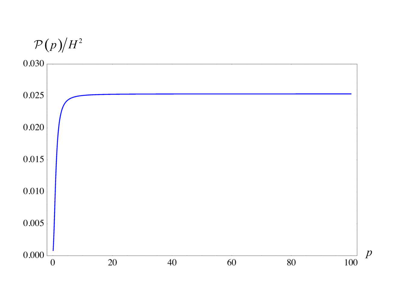
𝒫⁡(p)=H2​Z​p32​π2→p≫1(H2​π)2.\displaystyle{\cal P}(p)=H^{2}Z\,\frac{p^{3}}{2\pi^{2}}\,\xrightarrow{p\gg 1}\left(\frac{H}{2\pi}\right)^{2}\,. (2.52)

This is the well-known result for vacuum fluctuations after horizon exit. The spectrum as a function of pp is plotted in Figure 2.

Refer to caption
Figure 2: The spectrum of vacuum fluctuations for a massless scalar field as a function of pp.

3 Spectrum of quantum fluctuations using the reduced density matrix

In previous section, we discussed the spectrum of vacuum fluctuations by using the field operator expanded in terms of the mode functions defined for the Bunch-Davies vacuum. We next want to explore the spectrum of vacuum fluctuations by using the reduced density matrix derived by Maldacena and Pimentel in [7]. In this section, we first review the formalism to obtain the reduced density matrix and then discuss the spectrum of vacuum fluctuations.

3.1 A review on the reduced density matrix

In order to derive the reduced density matrix in the region LL, we need to trace over the degrees of freedom of the region RR. To make this procedure practically possible, the reduced density matrix has to be diagonalized. The following is a review on the derivation of the reduced density matrix given in [7].

As we see in Eq. (2.28), the mode function χI\chi^{I} corresponding to the Bunch-Davies vacuum is a linear combination of the Legendre functions PR,L=Pν−1/2i​p​(cosh⁡tR,L)P^{R,L}=P^{ip}_{\nu-1/2}(\cosh t_{R,L}), which are proportional to the positive frequency modes in the past in each RR or LL region. Setting τ=cosh⁡t\tau=\cosh t, the Legendre functions are known to be normalized as

(τ2−1)(dPq∗d​τPq−d​Pqd​τPq∗)=2​i​p|Γ⁡(1+i​p)|2,\displaystyle\left(\tau^{2}-1\right)\left(\frac{dP^{q*}}{d\tau}P^{q}-\frac{dP^{q}}{d\tau}P^{q*}\right)=\frac{2ip}{|\Gamma(1+ip)|^{2}}\,, (3.1)

where q=Rq=R or LL. Thus, the properly normalized positive frequency functions in each RR or LL region are given by

φq=Nb−1​Pq,Nb=2​p|Γ⁡(1+i​p)|.\displaystyle\varphi^{q}=N_{b}^{-1}P^{q}\,,\qquad N_{b}=\frac{\sqrt{2p}}{|\Gamma(1+ip)|}\,. (3.2)

Let us introduce φI\varphi^{I} as

φI=(φqφq∗).\displaystyle\varphi^{I}=\left(\begin{array}[]{l}\varphi^{q}\\ \varphi^{q*}\end{array}\right)\,.

Then this procedure of changing the mode functions from χI\chi^{I} to φI\varphi^{I} is a Bogoliubov transformation. The Bogoliubov coefficients are then expressed in terms of α\alpha and β\beta in the matrix MM in Eq. (2.1). So let us introduce new creation and anihilation operators bIb_{I} defined such that bR​|R⟩=0b_{R}|R\rangle=0 and bL​|L⟩=0b_{L}|L\rangle=0. Now, with the proper normalization in Eq. (3.2), the original field operator in Eq. (2.28) is expanded in terms of the new operators bJb_{J} as

ϕ⁡(t)=Hsinh⁡t​aI​χI=Hsinh⁡t​bJ​φJ,bJ=(bq,bq†),\displaystyle\phi(t)=\frac{H}{\sinh t}\,a_{I}\,\chi^{I}=\frac{H}{\sinh t}\,b_{J}\,\varphi^{J}\,,\qquad b_{J}=\left(\,b_{q}\,,\,b_{q}^{\dagger}\,\right)\,, (3.6)

where again the capital indices (I,J)(I,J) run from 1 to 4, q=(R,L)q=(R,L), and the repeated indices are summed over. By comparing Eqs. (2.28) and (3.6), the relation between the operators aIa_{I} and bIb_{I} has to be

aJ=NpNb−1bI(M−1)I,J(M−1)I=J(ξqσδqσδq∗σξq∗σ),{ξ=(α−β​α∗−1​β∗)−1,δ=−α−1​β​ξ∗.\displaystyle a_{J}=N_{p}\,N_{b}^{-1}\,b_{I}\left(M^{-1}\right)^{I}{}_{J}\,,\qquad\left(M^{-1}\right)^{I}{}_{J}=\left(\begin{array}[]{ll}\xi^{q}{}_{\sigma}&~\delta^{q}{}_{\sigma}\\ \delta^{q*}{}_{\!\!\sigma}&~\xi^{q*}{}_{\!\!\sigma}\\ \end{array}\right)\,,\qquad\left\{\begin{array}[]{l}\xi=\left(\alpha-\beta\,\alpha^{*\,-1}\beta^{*}\right)^{-1}\,,\\ \delta=-\alpha^{-1}\beta\,\xi^{*}\,.\end{array}\right.

Note that M−1M^{-1} is not normalized but its determinant is (|ξ|2−|δ|2)−1/2=(|α|2−|β|2)1/2\left(|\xi|^{2}-|\delta|^{2}\right)^{-1/2}=\left(|\alpha|^{2}-|\beta|^{2}\right)^{1/2}, which corresponds to Np​Nb−1N_{p}\,N_{b}^{-1} in Eq. (3.1). Thus, the Bunch-Davies vacuum can be regarded as a Bogoliubov transformation of the R,LR,L-vacua as

|BD⟩∝exp⁡(12​∑i,j=R,Lmi​j​bi†​bj†)​|R⟩​|L⟩,\displaystyle|{\rm BD}\rangle\propto\exp\left(\frac{1}{2}\sum_{i,j=R,L}m_{ij}\,b_{i}^{\dagger}\,b_{j}^{\dagger}\right)|R\rangle|L\rangle\,, (3.12)

where mi​jm_{ij} is a symmetric matrix and the operators bib_{i} satisfy the commutation relation [bi,bj†]=δi​j[b_{i},b_{j}^{\dagger}]=\delta_{ij}. Note that the normalization of the Bogoliubov transformation is omitted here for simplicity because it is unnecessary for the derivation of the reduced density matrix, which will be given in Eq. (3.27).

Here we mention a subtlety associated with the fact that the pp-mode spectrum is continuous. Since the commutation relation between the pp-mode annihilation operator and the p′p^{\prime}-mode creation operator is proportional to δ⁡(p−p′)\delta(p-p^{\prime}), that between the same spectral index p=p′p=p^{\prime} would diverge. To avoid this divergence, we discretize the pp-mode spectrum with a width Δ​p\Delta p and take the limit Δ​p→0\Delta p\to 0 only at the end of computation. This means, for example, we rescale the operators bib_{i} as bi→bi=Δ​p​bicontb_{i}\to b_{i}=\sqrt{\Delta p}\,b_{i}^{\rm cont}, where the index ‘cont’ denotes the operator with the original, continuous spectrum, and the operators bib_{i} and bjb_{j} appearing in Eq. (3.12) should be understood as the rescaled ones.

The condition aσ​|BD⟩=0a_{\sigma}|{\rm BD}\rangle=0 determines mi​jm_{ij}:

mi​j=−δi​σ∗​(ξ−1)σ​j=ei​θ​2​e−p​πcosh⁡2​π​p+cos⁡2​π​ν​(cos⁡π​νi​sinh⁡p​πi​sinh⁡p​πcos⁡π​ν),\displaystyle m_{ij}=-\delta_{i\sigma}^{*}\left(\xi^{-1}\right)_{\sigma j}=e^{i\theta}\frac{\sqrt{2}\,e^{-p\pi}}{\sqrt{\cosh 2\pi p+\cos 2\pi\nu}}\left(\begin{array}[]{cc}\cos\pi\nu&i\sinh p\pi\\ i\sinh p\pi&\cos\pi\nu\\ \end{array}\right)\,,

where ei​θe^{i\theta} contains all unimportant phase factors for ν2>0\nu^{2}>0.

When the state is written in the form of Eq. (3.12), it is still difficult to trace over the RR degrees of freedom because the density matrix ρ=|BD⟩​⟨BD|\rho=|{\rm BD}\rangle\langle{\rm BD}| is not diagonal in the |R⟩​|L⟩|R\rangle|L\rangle basis. Thus, we perform another Bogoliubov transformation further by introducing new operators cRc_{R} and cLc_{L}

cR=u​bR+v​bR†,cL=u¯​bL+v¯​bL†,\displaystyle c_{R}=u\,b_{R}+v\,b_{R}^{\dagger}\,,\qquad\quad c_{L}=\bar{u}\,b_{L}+\bar{v}\,b_{L}^{\dagger}\,, (3.16)

to obtain the relation

|BD⟩=Nγp−1​exp⁡(γp​cR†​cL†)​|R′⟩​|L′⟩.\displaystyle|{\rm BD}\rangle=N_{\gamma_{p}}^{-1}\exp\left(\gamma_{p}\,c_{R}^{\dagger}\,c_{L}^{\dagger}\,\right)|R^{\prime}\rangle|L^{\prime}\rangle\,. (3.17)

Here, the normalizaion |u|2−|v|2=1|u|^{2}-|v|^{2}=1 and |u¯|2−|v¯|2=1|\bar{u}|^{2}-|\bar{v}|^{2}=1 are assumed so that the new operators satisfy the commutation relation [ci,cj†]=δi​j[c_{i},c_{j}^{\dagger}]=\delta_{ij}. The normalization factor NγpN_{\gamma_{p}} is given by

Nγp2=|exp⁡(γp​cR†​cL†)​|R′⟩​|L′⟩|2=11−|γp|2,\displaystyle N_{\gamma_{p}}^{2}=\left|\exp\left(\gamma_{p}\,c_{R}^{\dagger}\,c_{L}^{\dagger}\,\right)|R^{\prime}\rangle|L^{\prime}\rangle\right|^{2}=\frac{1}{1-|\gamma_{p}|^{2}}\,, (3.18)

where |γp|<1|\gamma_{p}|<1 is imposed. Eq. (3.16) is a linear transformation between cqc_{q} and bqb_{q}, so this Bogoliubov transformation does not mix RR and LL Hilbert spaces, but the basis vacuum changes from |R⟩​|L⟩|R\rangle|L\rangle to |R′⟩​|L′⟩|R^{\prime}\rangle|L^{\prime}\rangle.

For later convenience, we introduce a 4×44\times 4 matrix form of Eq. (3.16),

cJ=bIGI,JGI=J(UqVq∗VqUq∗),cJ=(cq,cq†),\displaystyle c_{J}=b_{I}\,G^{I}{}_{J}\,,\qquad G^{I}{}_{J}=\left(\begin{array}[]{ll}U_{q}&~V_{q}^{*}\\ V_{q}&~U_{q}^{*}\\ \end{array}\right)\,,\qquad c_{J}=(c_{q}\,,c_{q}^{\dagger})\,,

where Uq≡diag⁡(u,u¯)U_{q}\equiv{\rm diag}(u,\bar{u}), Vq≡diag⁡(v,v¯)V_{q}\equiv{\rm diag}(v,\bar{v}).

The consistency conditions for Eq. (3.17) are

cR​|BD⟩=γp​cL†​|BD⟩,cL​|BD⟩=γp​cR†​|BD⟩.\displaystyle c_{R}\,|{\rm BD}\rangle=\gamma_{p}\,c_{L}^{\dagger}\,|{\rm BD}\rangle\,,\qquad c_{L}\,|{\rm BD}\rangle=\gamma_{p}\,c_{R}^{\dagger}\,|{\rm BD}\rangle\,. (3.22)

If we write mR​R=mL​L≡ωm_{RR}=m_{LL}\equiv\omega and mL​R=mR​L≡ζm_{LR}=m_{RL}\equiv\zeta in Eq. (3.1), we see that ω\omega is real and ζ\zeta is pure imaginary for positive ν2\nu^{2}. Then inserting Eqs. (3.12) and (3.16) into Eq. (3.22), we find a system of four homogeneous equations

ω​u+v−γp​ζ​v¯∗=0,ζ​u−γp​u¯∗−γp​ω​v¯∗=0,\displaystyle\omega\,u+v-\gamma_{p}\,\zeta\,\bar{v}^{*}=0\ ,\qquad\zeta\,u-\gamma_{p}\,\bar{u}^{*}-\gamma_{p}\,\omega\,\bar{v}^{*}=0\,, (3.23)
ω​u¯+v¯−γp​ζ​v∗=0,ζ​u¯−γp​u∗−γp​ω​v∗=0,\displaystyle\omega\,\bar{u}+\bar{v}-\gamma_{p}\,\zeta\,v^{*}=0\ ,\qquad\zeta\,\bar{u}-\gamma_{p}\,u^{*}-\gamma_{p}\,\omega\,v^{*}=0\,, (3.24)

where ω∗=ω\omega^{*}=\omega and ζ∗=−ζ\zeta^{*}=-\zeta. We see that setting v∗=v¯v^{*}=\bar{v} and u∗=u¯u^{*}=\bar{u} is possible if γp\gamma_{p} is pure imaginary γp∗=−γp\gamma_{p}^{*}=-\gamma_{p}. This is always possible by adjusting the phase of cqc_{q}. Then Eq. (3.24) becomes identical with Eq. (3.23) and the system is reduced to that of two homogeneous equations. We look for such γp\gamma_{p}, keeping the normalization condition |u|2−|v|2=1|u|^{2}-|v|^{2}=1 satisfied.

In order to have a non-trivial solution in the system of equations (3.23), γp\gamma_{p} must be

γp=12​ζ​[−ω2+ζ2+1−(ω2−ζ2−1)2−4​ζ2],\displaystyle\gamma_{p}=\frac{1}{2\zeta}\left[-\omega^{2}+\zeta^{2}+1-\sqrt{\left(\omega^{2}-\zeta^{2}-1\right)^{2}-4\zeta^{2}}\,\right]\,, (3.25)

where we took a minus sign in front of the square root term to satisfy |γp|<1|\gamma_{p}|<1. Note that γp\gamma_{p} is pure imaginary. Putting the ω\omega and ζ\zeta defined in Eq. (3.1) into Eq. (3.25), we get

γp=i​2cosh⁡2​π​p+cos⁡2​π​ν+cosh⁡2​π​p+cos⁡2​π​ν+2.\displaystyle\gamma_{p}=i\frac{\sqrt{2}}{\sqrt{\cosh 2\pi p+\cos 2\pi\nu}+\sqrt{\cosh 2\pi p+\cos 2\pi\nu+2}}\,. (3.26)

Now we have the density matrix which enables us to trace over the RR degrees of freedom easily. By using Eqs. (3.17) and (3.18), the reduced density matrix is then found to be diagonalized as

ρL=TrR|BD⟩⟨BD|=(1−|γp|2)∑n=0∞|γp|2​n|n;pℓm⟩⟨n;pℓm|,\displaystyle\rho_{L}={\rm Tr}_{R}\,|{\rm BD}\rangle\langle{\rm BD}|=\left(1-|\gamma_{p}|^{2}\,\right)\sum_{n=0}^{\infty}|\gamma_{p}|^{2n}\,|n;p\ell m\rangle\langle n;p\ell m|\,, (3.27)

where we defined |n;pℓm⟩=1/n!(cL†)n|L′⟩|n;p\ell m\rangle=1/\sqrt{n!}\,(c_{L}^{\dagger})^{n}\,|L^{\prime}\rangle. Note that this density matrix is for each mode labeled by p,ℓ,mp,\ell,m.

3.2 Spectrum of vacuum fluctuations

Now we calculate the mean-square vacuum fluctuations by using the reduced density matrix obtained in Eq. (3.27). Since we traced out the degrees of freedom of the RR region, the corresponding field operator has to be defined only in the LL region. Also the field operator should act only on |L′⟩|L^{\prime}\rangle conforming with the reduced density matrix. Then, the Fourier mode field operator should be defined as

ϕL​p​ℓ​m​(tL)≡ϕL​(tL)\displaystyle\phi_{Lp\ell m}(t_{L})\equiv\phi_{L}(t_{L}) =\displaystyle= 1Nb​Hsinh⁡tL​b𝒥​P𝒥=1Nb​Hsinh⁡tL​cℐ​(G−1)ℐ​P𝒥𝒥\displaystyle\frac{1}{N_{b}}\frac{H}{\sinh t_{L}}\,b_{\cal J}\,P^{\cal J}=\frac{1}{N_{b}}\frac{H}{\sinh t_{L}}\,c_{\cal I}\left(G^{-1}\right)^{\cal I}{}_{\cal J}\,P^{\cal J}
≡\displaystyle\equiv Hsinh⁡tL​cℐ​ψℐ,ψℐ=(ψLψL∗),\displaystyle\frac{H}{\sinh t_{L}}\,c_{\cal I}\,\psi^{\cal I}\,,\qquad\psi^{\cal I}=\left(\begin{array}[]{l}\psi^{L}\\ \psi^{L*}\end{array}\right)\,,

where the calligraphic indices (ℐ,𝒥)({\cal I,J}) run from 1 to 2, and the matrix is reduced to a 2×22\times 2 form:

(G−1)ℐ=𝒥(u¯∗−v¯∗−v¯u¯),|u¯|2−|v¯|2=1.\displaystyle\left(G^{-1}\right)^{\cal I}{}_{\cal J}=\left(\begin{array}[]{cc}\bar{u}^{*}&-\bar{v}^{*}\\ -\bar{v}&\bar{u}\\ \end{array}\right)\,,\qquad|\bar{u}|^{2}-|\bar{v}|^{2}=1\,.

Note that we transformed the field operator expanded by bJb_{J} in Eq. (3.6) into cIc_{I} by using Eq. (3.1)22 2 The Fourier mode field operator ϕL\phi_{L} is rescaled in accordance with the discretization of the pp-mode spectrum as explained below Eq. (3.12)..

Focusing on a single mode with indices p,ℓ,mp,\ell,m, the mean-square vacuum fluctuations are then calculated as

TrL​ρL​ϕL​ϕL†\displaystyle{\rm Tr}_{L}\rho_{L}\,\phi_{L}\,\phi_{L}^{\dagger} =\displaystyle= (1−|γp|2)​∑n=0∞|γp|2​n​⟨n;p​ℓ​m​|ϕL​ϕL†|​n;p​ℓ​m⟩,\displaystyle\left(1-|\gamma_{p}|^{2}\,\right)\sum_{n=0}^{\infty}|\gamma_{p}|^{2n}\langle n;p\ell m|\,\phi_{L}\,\phi_{L}^{\dagger}\,|n;p\ell m\rangle\,, (3.34)

where ϕL=ϕL​p​ℓ​m​(tL)\phi_{L}=\phi_{Lp\ell m}(t_{L}).

3.3 Spectrum in the LL region

We calculate the power spectrum in the LL region. The mode function given in Eq. (3.2) is written as

ψℐ=Nb−1​(G−1)ℐ​P𝒥𝒥=(𝒜LPL+ℬLPL∗ℬ∗LPL+𝒜∗LPL∗),\displaystyle\psi^{\cal I}=N_{b}^{-1}\left(G^{-1}\right)^{\cal I}{}_{\cal J}\,P^{\cal J}=\left(\begin{array}[]{l}{\cal A}_{L}P^{L}+{\cal B}_{L}P^{L*}\\ {\cal B}^{*}_{L}P^{L}+{\cal A}^{*}_{L}P^{L*}\end{array}\right)\,,

where we defined

𝒜L=u¯∗Nb,ℬL=−v¯∗Nb.\displaystyle{\cal A}_{L}=\frac{\bar{u}^{*}}{N_{b}}\,,\qquad{\cal B}_{L}=-\frac{\bar{v}^{*}}{N_{b}}\,. (3.38)

Here, u¯\bar{u}, v¯\bar{v} are obtained by solving Eq. (3.23) with the solution Eq. (3.26) and imposing the normalization condition |u¯|2−|v¯|2=1|\bar{u}|^{2}-|\bar{v}|^{2}=1:

u¯=1−γp​ζ|1−γp​ζ|2−|ω|2,v¯=ω|1−γp​ζ|2−|ω|2.\displaystyle\bar{u}=\frac{1-\gamma_{p}\zeta}{\sqrt{|1-\gamma_{p}\zeta|^{2}-|\omega|^{2}}}\,,\qquad\bar{v}=\frac{\omega}{\sqrt{|1-\gamma_{p}\zeta|^{2}-|\omega|^{2}}}\,. (3.39)

Here, ω=mR​R=mL​L\omega=m_{RR}=m_{LL} and ζ=mL​R=mR​L\zeta=m_{LR}=m_{RL} in Eq. (3.1). Using these we can compute the expectation value for each nn-particle state in Eq. (3.34),

⟨n;p​ℓ​m​|ϕL​ϕL†|​n;p​ℓ​m⟩\displaystyle\langle n;p\ell m|\,\phi_{L}\,\phi_{L}^{\dagger}\,|n;p\ell m\rangle =\displaystyle= 1n!​⟨L′|(cL)n​ϕL​ϕL†​(cL†)n|L′⟩\displaystyle\frac{1}{n!}\,\langle L^{\prime}|(c_{L})^{n}\,{\phi}_{L}\,{\phi}_{L}^{\dagger}\,(c_{L}^{\dagger})^{n}|L^{\prime}\rangle (3.40)
=\displaystyle= H2sinh2⁡tL​1n!​⟨L′|(cL)n​cℐ​ψℐ​(c𝒥​ψ𝒥)†​(cL†)n|L′⟩\displaystyle\frac{H^{2}}{\sinh^{2}t_{L}}\,\frac{1}{n!}\,\langle L^{\prime}|(c_{L})^{n}\,c_{\cal I}\,\psi^{\cal I}\,\left(c_{\cal J}\,\psi^{\cal J}\right)^{\dagger}\,(c_{L}^{\dagger})^{n}|L^{\prime}\rangle
=\displaystyle= H2sinh2⁡tL​|ψL|2​(2​n+1),\displaystyle\frac{H^{2}}{\sinh^{2}t_{L}}|\psi^{L}|^{2}\left(2n+1\right)\,,

where from the second line to the third line we used

⟨L′|(cL)n​cℐ​ψℐ​(c𝒥​ψ𝒥)†​(cL†)n|L′⟩\displaystyle\langle L^{\prime}|(c_{L})^{n}\,c_{\cal I}\,\psi^{\cal I}\,\left(c_{\cal J}\,\psi^{\cal J}\right)^{\dagger}\,(c_{L}^{\dagger})^{n}|L^{\prime}\rangle
=|ψL|2n!⟨n;pℓm|n;pℓm⟩+2|ψL|2n2(n−1)!⟨n−1;pℓm|n−1;pℓm⟩\displaystyle\qquad=|\psi^{L}|^{2}\,n!\,\langle n;p\ell m|n;p\ell m\rangle+2|\psi^{L}|^{2}\,n^{2}(n-1)!\,\langle n-1;p\ell m|n-1;p\ell m\rangle
=(2​n+1)​n!​|ψL|2.\displaystyle\qquad=(2n+1)\,n!\,|\psi^{L}|^{2}\,. (3.41)

Putting Eq. (3.40) into Eq. (3.34), the mean-square vacuum fluctuations for each mode is given by

TrL​ρL​ϕL​ϕL†\displaystyle{\rm Tr}_{L}\rho_{L}\,\phi_{L}\,\phi_{L}^{\dagger} =\displaystyle= H2sinh2⁡tL​|ψL|2​(1−|γp|2)​∑n=0∞|γp|2​n​(2​n+1)\displaystyle\frac{H^{2}}{\sinh^{2}t_{L}}|\psi^{L}|^{2}\left(1-|\gamma_{p}|^{2}\,\right)\sum_{n=0}^{\infty}|\gamma_{p}|^{2n}(2n+1) (3.42)
=\displaystyle= H2sinh2⁡tL​|ψL|2​1+|γp|21−|γp|2.\displaystyle\frac{H^{2}}{\sinh^{2}t_{L}}\,|\psi^{L}|^{2}\,\frac{1+|\gamma_{p}|^{2}}{1-|\gamma_{p}|^{2}}\,.

Note that by comparing with Eq. (2.38), we see the main effect of tracing out the degrees of freedom of the region RR seems to come in with the form of (1+|γp|2)/(1−|γp|2)(1+|\gamma_{p}|^{2})/(1-|\gamma_{p}|^{2}). Since |γp|→1|\gamma_{p}|\rightarrow 1 as p→0p\rightarrow 0 (for m=0m=0), this extra term enhances the mean-square vacuum fluctuations at long wavelengths (p≪1p\ll 1). Note also that the mode functions are changed from

χI=Np−1​MI​P𝒥𝒥⟶ψℐ=Nb−1​(G−1)ℐ​P𝒥𝒥,\displaystyle\chi^{I}=N_{p}^{-1}\,M^{I}{}_{\cal J}\,P^{\cal J}\,\longrightarrow\,\psi^{\cal I}=N_{b}^{-1}\left(G^{-1}\right)^{\cal I}{}_{\cal J}\,P^{\cal J}\,, (3.43)

due to the change from the Bunch-Davies vacuum to L′L^{\prime}-vacuum which diagonalized the reduced density matrix as obtained in Eq. (3.27).

3.4 Vacuum fluctuations after horizon exit

As we did in subsection 2.3, let us check the time dependence of ψℐ\psi^{\cal I} in Eq. (4.7). From Eq. (3.3), the |ψℐ|2|\psi^{\cal I}|^{2} in the mean-square vacuum fluctuations in Eq. (3.42) is expressed as

|ψL|2=𝒜LℬL∗(PL)2+(|𝒜L|2+|ℬL|2)PLPL∗+𝒜L∗ℬL(PL∗)2.\displaystyle|\psi^{L}|^{2}={\cal A}_{L}{\cal B}_{L}^{*}\left(P^{L}\right)^{2}+\left(|{\cal A}_{L}|^{2}+|{\cal B}_{L}|^{2}\right)P^{L}P^{L*}+{\cal A}_{L}^{*}{\cal B}_{L}\left(P^{L*}\right)^{2}\,. (3.44)

Since the Legendre functions on superhorizon scale is the same as in Eq. (2.46), we find the time dependence of this case is the same as Eq. (2.47) and expressed as

|ψL|2→tL≫122​ν−1​Γ​(ν)2π​[𝒜L​ℬL∗Γ​(ν−i​p+1/2)2+|𝒜L|2+|ℬL|2|Γ⁡(ν+i​p+1/2)|2+𝒜L∗​ℬLΓ​(ν+i​p+1/2)2]\displaystyle|\psi^{L}|^{2}\xrightarrow{t_{L}\gg 1}\frac{2^{2\nu-1}\Gamma(\nu)^{2}}{\pi}\left[\frac{{\cal A}_{L}{\cal B}_{L}^{*}}{\Gamma(\nu-ip+1/2)^{2}}+\frac{|{\cal A}_{L}|^{2}+|{\cal B}_{L}|^{2}}{|\Gamma(\nu+ip+1/2)|^{2}}+\frac{{\cal A}_{L}^{*}{\cal B}_{L}}{\Gamma(\nu+ip+1/2)^{2}}\right]
×(cosh⁡tL)2​ν−1\displaystyle\hskip 56.9055pt\times\left(\cosh t_{L}\right)^{2\nu-1}
≡𝒵​(cosh⁡tL)2​ν−1,\displaystyle\hskip 56.9055pt\equiv{\cal Z}\left(\cosh t_{L}\right)^{2\nu-1}\,, (3.45)

where we defined 𝒵{\cal Z} corresponding to ZZ in Eq. (2.47) for comparison. The spectrum of the vacuum fluctuations corresponding to Eq. (2.39) is now given by

𝒫⁡(p,tL)=p32​π2​TrL​ρL​ϕL​ϕL.\displaystyle{\cal P}(p,t_{L})=\frac{p^{3}}{2\pi^{2}}\,{\rm Tr}_{L}\rho_{L}\,\phi_{L}\,\phi_{L}\,. (3.46)

Plugging Eqs. (3.42) and (3.45) into above, we find the spectrum is found to be

𝒫⁡(p,tL)=H2sinh2⁡tL​|ψL|2​1+|γp|21−|γp|2​p32​π2→tL≫1H2​𝒵​1+|γp|21−|γp|2​p32​π2​(cosh⁡tL)2​ν−1sinh2⁡tL.\displaystyle{\cal P}(p,t_{L})=\frac{H^{2}}{\sinh^{2}t_{L}}\,|\psi^{L}|^{2}\,\frac{1+|\gamma_{p}|^{2}}{1-|\gamma_{p}|^{2}}\,\frac{p^{3}}{2\pi^{2}}\,\xrightarrow{t_{L}\gg 1}H^{2}{\cal Z}\,\frac{1+|\gamma_{p}|^{2}}{1-|\gamma_{p}|^{2}}\,\frac{p^{3}}{2\pi^{2}}\,\frac{(\cosh t_{L})^{2\nu-1}}{\sinh^{2}t_{L}}\,. (3.47)

We see the time dependent part is completely identical with Eq. (2.48). Thus, for massless case (ν=3/2\nu=3/2), the vacuum fluctuation gets frozen after horizon exit in the case of the spectrum using the reduced density matrix as well.

3.5 Wavenumber dependence

Next, let us see the behavior of the power spectrum at short wavelengths (p≫1p\gg 1) as we did in subsection 2.4. For a massless scalar field (ν=3/2\nu=3/2), the dominant term in 𝒵{\cal Z} of Eq. (3.45) for large pp is found to be

|𝒜L|2|Γ⁡(ν+i​p+1/2)|2=|u¯|2/|Nb|2|Γ⁡(ν+i​p+1/2)|2→p≫1π​e−π​p2​p4​|Γ⁡(i​p)|2.\displaystyle\frac{|{\cal A}_{L}|^{2}}{|\Gamma(\nu+ip+1/2)|^{2}}=\frac{|\bar{u}|^{2}/|N_{b}|^{2}}{|\Gamma(\nu+ip+1/2)|^{2}}\xrightarrow{p\gg 1}\frac{\pi e^{-\pi p}}{2p^{4}|\Gamma(ip)|^{2}}\,. (3.48)

The corresponding case of the Bunch-Davies vacuum is Eq. (2.50). We see the αLσ/Np\alpha_{L}^{\sigma}/N_{p} is simply replaced by u¯/Nb\bar{u}/N_{b}, and find that the behavior of 𝒵{\cal Z} is the same as that of ZZ,

𝒵→p≫122​Γ​(3/2)2π​π​e−π​p2​p4​|Γ⁡(i​p)|2∼12​p3.\displaystyle{\cal Z}\xrightarrow{p\gg 1}\frac{2^{2}\Gamma(3/2)^{2}}{\pi}\frac{\pi e^{-\pi p}}{2p^{4}|\Gamma(ip)|^{2}}\sim\frac{1}{2p^{3}}\,. (3.49)

Thus the spectrum of a massless scalar field after horizon exit is evaluated as

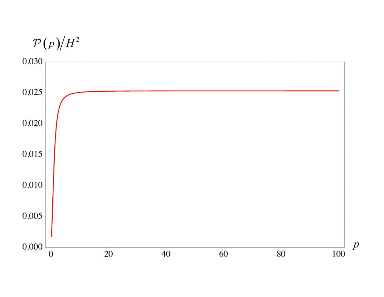
𝒫⁡(p)=H2​𝒵​1+|γp|21−|γp|2​(p32​π2)→p≫1(H2​π)2.\displaystyle{\cal P}(p)=H^{2}{\cal Z}\,\frac{1+|\gamma_{p}|^{2}}{1-|\gamma_{p}|^{2}}\left(\frac{p^{3}}{2\pi^{2}}\right)\xrightarrow{p\gg 1}\left(\frac{H}{2\pi}\right)^{2}\,. (3.50)

We find that the scale invariant spectrum is realized for p≫1p\gg 1 even after tracing out the degrees of freedom of the region RR. We plot the spectrum of the massless scalar field in Eq. (3.50) as a function of pp in Figure 3. It is almost identical to Figure 2.
Refer to caption
Figure 3: The spectrum as a function of pp.

4 Possible observable signatures

So far, we discussed two different spectra given in terms of χI\chi^{I} and ψℐ\psi^{\cal I}. The former correspond to the mode functions for the entangled  Bunch-Davies vacuum, and the latter to those that diagonalize the reduced density matrix obtained from the Bunch-Davies vacuum by tracing out the degrees of freedom of the RR region. The corresponding states are given by the density matrix ρBD=|BD⟩​⟨BD|\rho_{\rm BD}=|{\rm BD}\rangle\langle{\rm BD}| and the reduced density matrix ρL=TrR​ρBD\rho_{L}={\rm Tr}_{R}\,\rho_{\rm BD}, respectively.

The difference between these two states is the observer’s point of view when taking the mean-square vacuum fluctuations. For ρBD\rho_{\rm BD}, we are supposed to know the entangled state in the region RR. On the other hand, for ρL\rho_{L}, we are supposed to be completely ignorant about the state in the RR region. In order to distinguish them, we call ρBD\rho_{\rm BD} the “entangled state”, and ρL\rho_{L} the “mixed state (obtained from the entangled state)”, or just denote them by their relevant mode functions χI\chi^{I} and ψℐ\psi^{\cal I} in the following.

4.1 Non-entangled state

In the subsections 2.4 and 3.5, we showed that both of the entangled state and the mixed state realize the scale invariant spectrum for a massless scalar field at short wavelengths (p≫1p\gg 1). Now we wonder what would happen to the spectrum if we assume the LL region were the whole universe and use the mode function φℐ\varphi^{\cal I} which is defined only in the LL region. We call it “non-entangled state”, and denote it by φℐ\varphi^{\cal I}.

The relevant mode function for the non-entangled case should be given by Eq. (3.2). That is

φℐ=(φLφL∗)=1Nb​(PLPL∗).\displaystyle\varphi^{\cal I}=\left(\begin{array}[]{l}\varphi^{L}\\ \varphi^{L*}\end{array}\right)=\frac{1}{N_{b}}\left(\begin{array}[]{l}P^{L}\\ P^{L*}\end{array}\right)\,.

The spectrum is then defined by

𝒫⁡(p,tL)=p32​π2​⟨L|φL​φL|L⟩,\displaystyle{\cal P}(p,t_{L})=\frac{p^{3}}{2\pi^{2}}\,\langle L|\,\varphi^{L}\varphi^{L}\,|L\rangle\,, (4.6)

where the Fourier mode field operator is

φL​(tL)\displaystyle\varphi^{L}(t_{L}) =\displaystyle= Hsinh⁡t​bℐ​φℐ​(tL),\displaystyle\frac{H}{\sinh t}\,b_{\cal I}\,\varphi^{\cal I}(t_{L})\,, (4.7)

and we find the mean-square vacuum fluctuations for each mode

⟨L|φL​φL|L⟩=H2sinh2⁡tL​|φL|2​δ​(p−p′)​δℓ​ℓ′​δm​m′.\displaystyle\langle L|\,\varphi^{L}\varphi^{L}\,|L\rangle=\frac{H^{2}}{\sinh^{2}t_{L}}|\varphi^{L}|^{2}\,\delta(p-p^{\prime})\delta_{\ell\ell^{\prime}}\delta_{mm^{\prime}}\,. (4.8)

The |φL|2|\varphi^{L}|^{2} becomes a simple form

|φL|2=12​p​|Γ⁡(1+i​p)|2​PL​P∗L\displaystyle|\varphi^{L}|^{2}=\frac{1}{2p}\left|\Gamma(1+ip)\right|^{2}P^{L}P^{*L}
→tL≫122​ν−1​Γ​(ν)2π​|Γ⁡(1+i​p)|2|Γ⁡(ν+i​p+1/2)|2​12​p​(cosh⁡tL)2​ν−1≡𝒵~​(cosh⁡tL)2​ν−1.\displaystyle\hskip 28.45274pt\xrightarrow{t_{L}\gg 1}\frac{2^{2\nu-1}\Gamma(\nu)^{2}}{\pi}\frac{|\Gamma(1+ip)|^{2}}{|\Gamma(\nu+ip+1/2)|^{2}}\frac{1}{2p}\left(\cosh t_{L}\right)^{2\nu-1}\equiv\tilde{\cal Z}\left(\cosh t_{L}\right)^{2\nu-1}\,. (4.9)

Here, time independent part of 𝒵~\tilde{\cal Z} at short wavelengths (p≫1p\gg 1) is evaluated as

𝒵~→p≫122​Γ​(3/2)2π​|Γ⁡(1+i​p)|2|Γ⁡(2+i​p)|2​12​p∼12​p3.\displaystyle\tilde{\cal Z}\xrightarrow{p\gg 1}\frac{2^{2}\Gamma(3/2)^{2}}{\pi}\frac{|\Gamma(1+ip)|^{2}}{|\Gamma(2+ip)|^{2}}\frac{1}{2p}\sim\frac{1}{2p^{3}}\,. (4.10)

The power spectrum becomes

𝒫⁡(p)=H2​𝒵~​p32​π2→p≫1(H2​π)2.\displaystyle{\cal P}(p)=H^{2}\tilde{\cal Z}\,\frac{p^{3}}{2\pi^{2}}\,\xrightarrow{p\gg 1}\left(\frac{H}{2\pi}\right)^{2}\,. (4.11)

Thus, for p≫1p\gg 1, we get the flat spectrum of vacuum fluctuations for a massless scalar field even for the non-entangled state. This means that we cannot distinguish which state is valid for our universe as far as we focus on the short wavelength region of the spectrum. So let us examine the behavior at long wavelengths after the horizon exit.

4.2 Spectra at long wavelengths

In order to see the behavior at long wavelengths, we take the limit p≪1p\ll 1 and expand the expressions for the spectra in pp. For φℐ\varphi^{\cal I} and χI\chi^{I}, we expand 𝒵~\tilde{\cal Z} in Eq. (4.9) and ZZ in Eq. (2.47), respectively. Then we find the pp dependence at leading order is given by

𝒫⁡(p)→p≪1tL≫1{22​ν−1​Γ​(ν)2​π−1​|Γ⁡(ν+1/2)|−2​(H2​π)2​p2forφℐ,22​ν−1​Γ​(ν)2​|Γ⁡(ν+1/2)|−2​(H2​π)2​p3forχI.\displaystyle{\cal P}(p)\xrightarrow[p\ll 1]{t_{L}\gg 1}\left\{\begin{array}[]{l}2^{2\nu-1}\Gamma(\nu)^{2}\pi^{-1}|\Gamma(\nu+1/2)|^{-2}\left(\frac{H}{2\pi}\right)^{2}p^{2}\hskip 39.83368pt{\rm for}\quad\varphi^{\cal I}\,,\\ \\ 2^{2\nu-1}\Gamma(\nu)^{2}|\Gamma(\nu+1/2)|^{-2}\left(\frac{H}{2\pi}\right)^{2}p^{3}\,\hskip 56.9055pt{\rm for}\quad\chi^{I}\,.\end{array}\right.

In the case of ψℐ\psi^{\cal I}, we expand 𝒵\cal Z in Eq. (3.45) to obtain

𝒫⁡(p)→p≪1tL≫122​ν−1​Γ​(ν)2​2​π−2​|Γ⁡(ν+1/2)|−2​|cos⁡π​ν|​(1+cos⁡2​π​ν+3+cos⁡2​π​ν)\displaystyle\hskip-14.22636pt{\cal P}(p)\xrightarrow[p\ll 1]{t_{L}\gg 1}2^{2\nu-1}\Gamma(\nu)^{2}\,\sqrt{2}\,\pi^{-2}\,|\Gamma(\nu+1/2)|^{-2}\,|\cos\pi\nu|\left(\sqrt{1+\cos 2\pi\nu}+\sqrt{3+\cos 2\pi\nu}\right)
×(1+cos⁡2​π​ν+3+cos⁡2​π​ν)2+2(1+cos⁡2​π​ν+3+cos⁡2​π​ν)2−2​(H2​π)2​pforψℐ.\displaystyle\hskip 56.9055pt\times\frac{(\sqrt{1+\cos 2\pi\nu}+\sqrt{3+\cos 2\pi\nu})^{2}+2}{(\sqrt{1+\cos 2\pi\nu}+\sqrt{3+\cos 2\pi\nu})^{2}-2}\left(\frac{H}{2\pi}\right)^{2}p\,\hskip 42.67912pt{\rm for}\quad\psi^{\cal I}\,. (4.16)

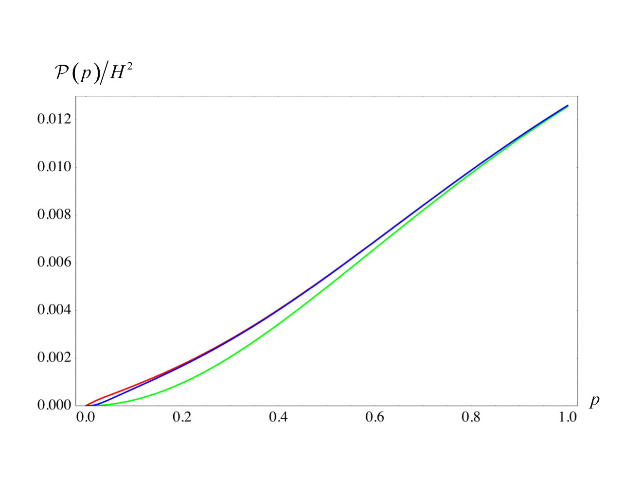
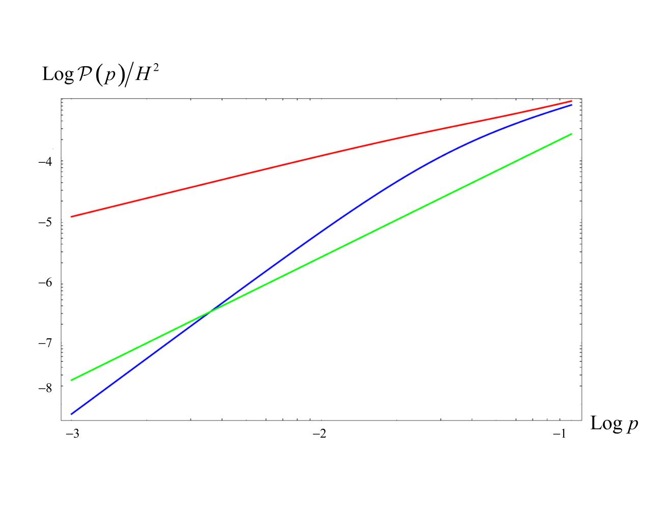
We are interested in the case of small mass (|ν−3/2|≪1|\nu-3/2|\ll 1). Taking this limit, we see that the spectrum for ψℐ\psi^{\cal I} decreases most slowly as p→0p\rightarrow 0. The spectra at long wavelengths are plotted in Figure 4, where we take m2=H2/10m^{2}=H^{2}/10. The spectra for the entangled state (χI\chi^{I}) and the mixed state (ψℐ\psi^{\cal I}) are the blue line and the red line, respectively. The green line is the spectrum for the non-entangled state (φℐ\varphi^{\cal I}). The non-entangled state seems to give the most suppressed spectrum at p≪1p\ll 1. But if we use the logarithmic plots (right panel) we find the result is consistent with the analysis of the pp dependence in Eqs. (4.2) and (4.16).

Around the curvature scale of the open universe (p∼1)(p\sim 1), we find that the green line starts to deviate from other two lines as p→0p\rightarrow 0. This point tells us if the regions RR and LL are entangled or not. Around 55 times of the curvature scale of the open universe (p∼0.2)(p\sim 0.2), the red and blue lines start to bifurcate. This tells us which state among the entangled state and the mixed state is appropriate for our universe.
Refer to caption
Refer to caption
Figure 4: The spectrum at long wavelengths (Left) and the logarithmic plot at very long wavelengths (Right). The red line is for ψℐ\psi^{\cal I}, the blue line is for χI\chi^{I}, and the green is for φℐ\varphi^{\cal I}.

5 Summary and discussion

We investigated the spectrum of vacuum fluctuations with quantum entanglement in de Sitter space by using the reduced density matrix obtained by Maldacena and Pimentel in [7]. We formulated the mean-square vacuum fluctuations by introducing the two open charts, LL and RR, which are entangled. We found that the effect of tracing out the degrees of freedom of the RR region comes in to the mean-square of vacuum fluctuations and enhances it on scales larger than the curvature radius. On the other hand, on small scales, the spectrum of vacuum fluctuations of a massless scalar field is found to be scale invariant, and completely indistinguishable from the pure Bunch-Davies (hence highly entangled) case.

We also considered a fictitious case in which we assume the LL region were the whole universe. In this case, with respect to a natural vacuum state defined in the LL region, the scale invariant spectrum is also realized on small scales. Thus it turned out that we cannot distinguish which state is valid for our universe among the entangled state (χI\chi^{I}), the mixed state from the entangled state (ψℐ\psi^{\cal I}) and non-entangled state (φℐ\varphi^{\cal I}), as long as we focus on the spectrum on small scales.

On the other hand, the spectrum for each of these three cases is found to be different from each other on large scales comparable to or greater than the curvature radius.

We found that the spectra for the entangled and mixed states tend to be enhanced compared to the non-entangled state on scales comparable to the curvature radius. If we go further to scales much larger than the curvature radius, there appears a difference between the entangled state and mixed state. The spectrum for the mixed state is enhanced substantially relative to the entangled state. Since we can use these differences to distinguish those three states, they seem to be relevant (and hopefully observationally testable) in the context of open inflation.

Now let us consider why the difference appeared in the spectra between the entangled and mixed states. In general, if we consider two subsystems AA and BB that form a state |Ψ⟩|\Psi\rangle, the expectation value of a physical quantity 𝒪{\cal O} is expressed by using the density matrix ρ=|Ψ⟩​⟨Ψ|\rho=|\Psi\rangle\langle\Psi| as

Trρ𝒪=∑α,β⟨α,β|Ψ⟩⟨Ψ|𝒪|α,β⟩=⟨Ψ|𝒪|Ψ⟩.\displaystyle{\rm Tr}\rho\,{\cal O}=\sum_{\alpha,\beta}\langle\alpha,\beta|\Psi\rangle\langle\Psi|{\cal O}|\alpha,\beta\rangle=\langle\Psi|{\cal O}|\Psi\rangle\,. (5.1)

If 𝒪{\cal O} depends only on AA, that is, 𝒪A{\cal O}_{A} :

⟨α′,β′​|𝒪|​α,β⟩=⟨α|𝒪A|α′⟩​δβ​β′,\displaystyle\langle\alpha^{\prime},\beta^{\prime}|{\cal O}|\alpha,\beta\rangle=\langle\alpha|{\cal O}_{A}|\alpha^{\prime}\rangle\delta_{\beta\beta^{\prime}}\,, (5.2)

then Eq. (5.1) becomes

Tr​ρ​𝒪A\displaystyle{\rm Tr}\rho\,{\cal O}_{A} =\displaystyle= ∑α,β∑α′,β′⟨α,β⁡|Ψ⟩​⟨Ψ|​α′,β′⟩​⟨α′,β′​|𝒪A|​α,β⟩=∑α,β∑α′⟨α,β⁡|Ψ⟩​⟨Ψ|​α′,β⟩​⟨α′​|𝒪A|​α⟩\displaystyle\sum_{\alpha,\beta}\sum_{\alpha^{\prime},\beta^{\prime}}\langle\alpha,\beta|\Psi\rangle\langle\Psi|\alpha^{\prime},\beta^{\prime}\rangle\langle\alpha^{\prime},\beta^{\prime}|{\cal O}_{A}|\alpha,\beta\rangle=\sum_{\alpha,\beta}\sum_{\alpha^{\prime}}\langle\alpha,\beta|\Psi\rangle\langle\Psi|\alpha^{\prime},\beta\rangle\langle\alpha^{\prime}|{\cal O}_{A}|\alpha\rangle (5.3)
=\displaystyle= Tr​ρA​𝒪A,\displaystyle{\rm Tr}\rho_{A}\,{\cal O}_{A}\,,

where

ρA≡TrB​ρ=∑α,α′|α⟩​(∑β⟨α,β⁡|Ψ⟩​⟨Ψ|​α′,β⟩)​⟨α′|.\displaystyle\rho_{A}\equiv{\rm Tr}_{B}\rho=\sum_{\alpha,\alpha^{\prime}}|\alpha\rangle\left(\sum_{\beta}\langle\alpha,\beta|\Psi\rangle\langle\Psi|\alpha^{\prime},\beta\rangle\right)\langle\alpha^{\prime}|\,. (5.4)

Thus, the expectation value Tr​ρ​𝒪{\rm Tr}\rho\,{\cal O} is equal to Tr​ρA​𝒪A{\rm Tr}\rho_{A}\,{\cal O}_{A} if 𝒪{\cal O} does not depend on BB. In other words, for an operator with the property 𝒪=𝒪A{\cal O}={\cal O}_{A}, the expectation value should agree with each other.

Based on this general argument, we may understand the reason why the spectra for the entangled state and the mixed state from the entangled state become different on large scale (p→0)(p\rightarrow 0). We see that the creation and anihilation operators aJa_{J} include the operators on both sides, bJ=(bq,bq†)b_{J}=(b_{q},b_{q}^{\dagger}) (q=R,Lq=R,L), as in Eq. (3.1). This means that the field operator ϕ⁡(t)\phi(t) naturally involves operators on both sides even if the time slice tt is restricted to the LL region. On the other hand, after tracing out the degrees of freedom of the RR region, the mixed state (ψℐ)(\psi^{\cal I}) is described by the creation and anihilation operators defined only in the LL region. That is, the field operator ϕL​(t)\phi_{L}(t) is defined only in the LL region. Thus apparently ϕ​(t)≠ϕL​(t)\phi(t)\neq\phi_{L}(t), implying that the above general argument does not hold because 𝒪≠𝒪A{\cal O}\neq{\cal O}_{A}.

Finally, we mention that it would be easy to extend our analysis to the case of gravitons. Another direction is to consider interactions. The formalism we developed in this paper is at tree level. It would be interesting to consider the loop corrections and see how they affect the result. They might enhance the effect of the entanglement on small scales because of the coupling between long and short wavelengths [19].

Acknowledgments

I would like to thank Jiro Soda and Misao Sasaki for fruitful discussions, and for helpful suggestions and comments. I would also like to thank Alex Vilenkin and Jaume Garriga for careful reading of the draft, and for very useful suggestions and comments. This work was supported in part by funding from the University Research Council of the University of Cape Town.

References

  • [1] S. R. Coleman and F. De Luccia, Phys. Rev. D 21, 3305 (1980).
  • [2] J. Garriga, S. Kanno, M. Sasaki, J. Soda and A. Vilenkin, JCAP 1212, 006 (2012) [arXiv:1208.1335 [hep-th]].
  • [3] J. Garriga, S. Kanno and T. Tanaka, JCAP 1306, 034 (2013) [arXiv:1304.6681 [hep-th]].
  • [4] M. B. Fröb, J. Garriga, S. Kanno, M. Sasaki, J. Soda, T. Tanaka and A. Vilenkin, JCAP 1404, 009 (2014) [arXiv:1401.4137 [hep-th]].
  • [5] S. Ryu and T. Takayanagi, Phys. Rev. Lett. 96, 181602 (2006) [hep-th/0603001].
  • [6] T. Takayanagi, Class. Quant. Grav. 29, 153001 (2012) [arXiv:1204.2450 [gr-qc]].
  • [7] J. Maldacena and G. L. Pimentel, JHEP 1302, 038 (2013) [arXiv:1210.7244 [hep-th]].
  • [8] S. Kanno, J. Murugan, J. P. Shock and J. Soda, arXiv:1404.6815 [hep-th].
  • [9] N. Iizuka, T. Noumi and N. Ogawa, arXiv:1404.7487 [hep-th].
  • [10] M. Sasaki, T. Tanaka and K. Yamamoto, Phys. Rev. D 51, 2979 (1995) [gr-qc/9412025].
  • [11] M. Bucher, A. S. Goldhaber and N. Turok, Phys. Rev. D 52, 3314 (1995) [hep-ph/9411206].
  • [12] A. D. Linde, Phys. Lett. B 351, 99 (1995) [hep-th/9503097].
  • [13] A. D. Linde and A. Mezhlumian, Phys. Rev. D 52, 6789 (1995) [astro-ph/9506017].
  • [14] J. Garriga, X. Montes, M. Sasaki and T. Tanaka, Nucl. Phys. B 513, 343 (1998) [astro-ph/9706229].
  • [15] J. Garriga, X. Montes, M. Sasaki and T. Tanaka, Nucl. Phys. B 551, 317 (1999) [astro-ph/9811257].
  • [16] T. S. Bunch and P. C. W. Davies, Proc. Roy. Soc. Lond. A 360, 117 (1978).
  • [17] N. A. Chernikov and E. A. Tagirov, Annales Poincare Phys. Theor. A 9, 109 (1968).
  • [18] J. B. Hartle and S. W. Hawking, Phys. Rev. D 28, 2960 (1983).
  • [19] T. Tanaka and Y. Urakawa, Class. Quant. Grav. 30, 233001 (2013) [arXiv:1306.4461 [hep-th]].