Quasi-exceptional domains

A domain $D\in{\mathbb{R}}^{n}$ is called exceptional if there is a positive function $u$ (called a roof function) harmonic in $D$, zero on the boundary, and

where the differentiation is along the normal pointing inwards into $D$, and it is assumed that the boundary is smooth. Evident examples are exteriors of balls and half-spaces. For $n>2$ the only other known examples are cylinders whose base is an exceptional domain in ${\mathbb{R}}^{2}$. If the smoothness assumption on the boundary is dropped, then there are also certain cones in higher dimensions and pathological “non-Smirnov” examples in the plane [11].

The problem of description of all exceptional domains in the plane was stated in [10] and settled in [11] under a topological assumption which was removed in [18] using an unexpected correspondence to minimal surfaces. The first non-trivial example was given in [10]. This example appeared in another context related to fluid dynamics in [13]. A second non-trivial example was noticed in [11] and [18]. This example had also appeared previously in studies of fluid dynamics [3] (see also [6]).

Let us introduce quasi-exceptional domains, by relaxing the definition to allow the Dirichlet condition to be a different constant on each boundary component. Thus, a domain $D\in{\mathbb{R}}^{n}$ is called quasi-exceptional if there is a positive harmonic function $u$ in $D$, which is constant on each boundary component (but not necessarily the same constant) and the Neumann condition (1) holds (with the same constant on each boundary component). We will continue to call $u$ a roof function. Again, we assume that each component of the boundary is smooth.

We summarize several interesting aspects of exceptional domains. These statements all hold true for quasi-exceptional domains except the last one:

• •

  Fluid dynamics: As noted above, the two non-trivial examples first appeared in fluid dynamics [13, 3]. In general, one can interpret exceptional domains in terms of a hollow vortex problem. The level lines of $u$ can be interpreted as stream lines of a two-dimensional stationary flow of ideal fluid, and condition (1) expresses the fact that the pressure is constant on the boundary. Such conditions may exist if the components of the complement of $D$ are air bubbles in the surrounding liquid. Notice that the rotation of the fluid around all bubbles corresponding to exceptional domains is in the same direction. This reflects our condition that $\partial_{n}u>0$.

• •

  Quadrature domains [8]: Exceptional domains provide examples of arclength null-quadrature domains, that is, domains for which integration over $\partial D$ of every analytic function in the Smirnov class $E^{1}(D)$ vanishes.

• •

  Differentials on Riemann surfaces: By way of the connection to quadrature domains, the study [8] indicates a connection to half-order differentials. We make use of Abelian differentials in Section 4 below.

• •

  The Schwarz function of a curve: In [11], it was noticed that the function $u(z)$ satisfies

  $$\partial_{z}u(z)=\sqrt{-S^{\prime}(z)},$$

  where $S(z)$ is the Schwarz function of $\partial\Omega$ and $\partial_{z}=\frac{1}{2}(\partial_{x}-i\partial_{y})$ is the Cauchy-Riemann operator.

• •

  Minimal surfaces: The recent work [18] established a nontrivial correspondence between exceptional domains and a special type of complete embedded minimal surfaces called a “minimal bigraphs”. This correspondence does not extend to quasi-exceptional domains.

The classification results for exceptional domains show that they are quite restricted; all examples can be conformally mapped from a disk by elementary functions.

We begin to address this problem below, give a partial classification of periodic and finitely-connected exceptional domains, and provide new periodic and doubly-connected examples described in terms of elliptic functions. First, we explain the relation to arclength null-quadrature domains.

A bounded domain $D\subset{\mathbb{C}}$ is a quadrature domain if it admits a formula expressing the area integral of every function $f$ analytic and integrable in $D$ as a finite sum of weighted point evaluations of the function and its derivatives. i.e.

where $z_{m}$ are distinct points in $D$ and $a_{m,k}$ are constants independent of $g$.

A (necessarily unbounded) domain $D\subset{\mathbb{C}}$ is called a null-quadrature domain (NQD) if the area integral of every function $g$ analytic and integrable in $D$ vanishes:

M. Sakai [17] completely classified NQDs in the plane.

Following [11] we will refer to a domain $D\subset{\mathbb{C}}$ as an arclength null-quadrature domain (ALNQD) if the integral over $\partial D$ of every function $g$ in the Smirnov class $E^{1}(D)$ vanishes (in the case $\infty$ is an isolated point on $\partial D$, we take the restricted class of functions $g(z)\in E^{1}(D)$ vanishing at infinity):

The Smirnov class $E^{1}(D)$ is not the same as the Hardy space $H^{1}(D)$. Namely, a function $g$ analytic in $D$ is said to belong to $E^{1}(D)$ if there exists a sequence of cycles $\gamma_{k}$ homologous to zero, rectifiable, and converging to the boundary $\partial D$ (in the sense that $\gamma_{k}$ eventually surrounds each compact sub-domain of $D$), such that:

One may also define quadrature domains in higher dimensions using a test class of harmonic functions, but we will restrict ourselves to the case of $n=2$ dimensions.

Inspired by the successful classification of NQDs [17], the problem of classifying ALNQDs was suggested in [11]. We pose this problem again while stressing that it does not reduce to the classification of exceptional domains (whereas it might reduce to classification of quasi-exceptional domains).

The following proposition shows that quasi-exceptional domains are ALNQDs. Thus, the new examples (described in the last section) of quasi-exceptional domains also provide new ALNQDs. Problem 2 is closely related to Problem 1, and if the converse of the proposition is true then the two problems are equivalent.

Suppose that $g$ is in the Smirnov space $E^{1}(D)$, and let $\phi$ be a conformal map to $D$ from a circular $\Omega$. Using the fact that $ds=iF(z)dz$, we have

Now $g(z)\in E^{1}(D)$ implies [7] that

unless $\infty$ is an isolated boundary point (in which case $g(\phi(\zeta))\phi^{\prime}(\zeta)$ need not be analytic at $\phi^{-1}(\infty)$). In the case $\infty$ is not an isolated boundary point, since $F(\phi(\zeta))$ is bounded (by the Claim), we have

and therefore, by Cauchy’s theorem, (5) vanishes. In the case $\infty$ is an isolated boundary point of $D$, $g(\phi(\zeta))\phi^{\prime}(\zeta)$ need not be analytic at $\zeta=\phi^{-1}(\infty)$. In fact it can have a pole up to order two. However, $F(z)=O(|z|^{-1})$ vanishes to order one at infinity by Bôcher’s Theorem (cf. [11, Thm. 3.1]). Thus, if $g(z)$ also vanishes at infinity then $g(\phi(\zeta))\phi^{\prime}(\zeta)F(\phi(\zeta))\in E^{1}(\Omega)$ and the previous argument follows. This shows that if $z\in D$ then $D$ is an ALNQD for the restricted class of functions $g(z)\in E^{1}(D)$ which vanish at infinity.

We restrict ourselves to the case $n=2$, and assume that the order of connectivity of $D$ is finite, or that the roof function $u$ is periodic, and the fundamental region for $D$ has finite connectivity.

Recall that a Martin function is a positive harmonic function $M$ in a domain $\Omega$ with the property that for any positive harmonic function $v$ in $\Omega$, the condition $v\leq M$ implies that $v=cM$, where $c>0$ is a constant. (Often, Martin functions are called minimal harmonic functions - cf. [9].) Martin functions on finitely connected domains are simply Poisson kernels evaluated at points of the Martin boundary, the boundary under Caratheodory compactification (prime ends) of the domain (see [4]).

Any domain $D$ of finite connectivity in ${\mathbb{C}}$ is conformally equivalent to a circular $\Omega$, whose boundary components are circles and points. For a circular, a Martin function $M$ can be of two types:

a) There is a component of $\partial\Omega$ which is a single point $z_{0}$, and $M$ is proportional to the Green function of $\Omega\cup\{z_{0}\}$ with the singularity at $z_{0}$.

b) There is a point $z_{0}\in\partial\Omega$ which is not a component of $\partial\Omega$, and $M$ has zero boundary values at all points of $\partial\Omega\backslash\{z_{0}\}.$ The local behavior in this case is like $-\mathrm{Im}\,(1/z)$ in the upper half-plane near $0$.

Let $D$ be an exceptional domain, and $u$ a harmonic function with the property (1). The following result was proved for exceptional domains by the current first author, but communicated in [11, Thm. 4.2]. Here we repeat the proof with minor adjustments.

Proof. We follow the second part of the proof from [11, Thm. 4.2].

Let $R>0$ and consider an auxiliary function

where $R>0$ is a parameter. A direct computation shows that

and $w_{R}(z)=1/(c_{k}+R)\leq 1/R$ for $z\in\partial D$, where $c_{k}\geq 0$ are the constants taken in the Dirichlet condition. We claim that

from which the result follows by letting $R\rightarrow\infty$ which gives $|\nabla u|\leq 2$ in $D$.

Suppose, contrary to (7), that $w_{R}(z_{0})>2/R,$ for some $z_{0}\in D$. Let

Obviously, $v(z)\geq 2/R$. A computation reveals that $\Delta\log v=v^{2}.$ Let

We have $z_{0}\in K$, since $v(z_{0})=2/R$. Let $K_{0}$ be the component of $K$, containing $z_{0}$. Then we have $w_{R}(z)=v(z)$ on $\partial K_{0}$, since $w_{R}(z)<v(z)$ on $\partial D\cap B(z_{0},R)$ while $v(z)=+\infty$ on $\partial B(z_{0},R)$. On the other hand,

So the subharmonic function $\log w_{R}-\log v$ is positive in $K_{0}$ and vanishes on the boundary, a contradiction.

This proves that $\nabla u=O(1)$. In order to see the second statement, we note that $\nabla u=O(1)$ implies that $u(z)=O(|z|)$ has order one. The result then follows by first solving the Dirichlet problem (with a bounded function) having the same boundary values as $u$; subtracting this function, one may then apply [12, Theorem II].

Let $D$ be a QE domain of one of the following types:

Type I. $D$ is finitely connected, or

Type II. $D/\Gamma$ is finitely connected, where $\Gamma$ is the group of transformations $z\mapsto z+n\omega$, and $u(z+\omega)=u(z)$ for some $\omega\in{\mathbb{C}}\backslash\{0\}$. We call this the periodic case. (As above, $u$ is the roof function.)

In this section we give a classification of QE domains of these two types in terms of Abelian differentials of a compact Riemann surface with an anti-conformal involution.

If $D$ is of type I, and $\infty$ is an isolated boundary point, then $D^{\prime}=D\cup\{\infty\}$ is conformally equivalent to some bounded circular domain $\Omega$, and we suppose that $p\in\Omega$ corresponds to $\infty$. If $\infty$ is not isolated, we put $D^{\prime}=D$, and $\Omega$ is a bounded circular domain conformally equivalent to $D^{\prime}$. In any case, we have a conformal map $\phi:\Omega\to D^{\prime}$.

If $D$ is of type II, let $G=D/\Gamma$. The Riemann surface $G$ is a finitely connected domain on the cylinder ${\mathbb{C}}/\Gamma$; this cylinder is conformally equivalent to the punctured plane; $G$ must have one or two punctures of ${\mathbb{C}}/\Gamma$ as isolated boundary points, and we denote by $G^{\prime}$ the union of $G$ with these isolated boundary points. Then $G^{\prime}$ is conformally equivalent to a bounded circular domain of finite connectivity $\Omega$ and we have a multi-valued conformal map $\phi:\Omega\to G^{\prime}$. Let $a$ and $b$ denote the one or two points in $\Omega$ that correspond to the added punctures of $G^{\prime}$.

In all cases $a$ and $b$ are simple poles of $\phi$.

We pull back $u$ on $\Omega:$ set $v=u\circ\phi$. As $u$ is periodic, $v$ is a single-valued positive harmonic function on $\Omega\backslash\{a,b\}$.

Consider the differential on $\Omega$

This is well defined on $\Omega$: $g$ is a single-valued meromorphic function in $\Omega$ with simple poles exactly at $a$ and $b$ (if any of these points is present in $\Omega$).

Next, we extend $v$ as a multi-valued function to a compact Riemann surface $S$. Let $\Omega^{\prime}$ be the mirror image of $\Omega$; we glue it to $\Omega$ in the standard way (along each circular boundary component) and obtain a compact Riemann surface $S$. We denote by $\sigma:z\mapsto z^{*}$ the anti-conformal involution which fixes the boundary components of $\Omega$. The Riemann surface $S$ is of genus $g$, and the involution $\sigma$ has fixed set corresponding to $\partial\Omega$, which consists of $n=g+1$ ovals. Such involutions are called involutions of maximal type.

Each branch of $v$ is constant on each boundary component, so it extends through this boundary component by reflection to the double $S$ of $\Omega$. The extensions of various branches of $v$ through different boundary components do not match: they differ by additive constants. On the other hand, the differential $dv$ is well defined on the double. Namely,

where $*$ is the action of involution on differentials. Thus we have a meromorphic differential $dv$ on $S$.

Choose a basis of $1$-homology in $S$ so that the $A$-loops are simple closed curves in $\Omega$, each homotopic to one boundary component of $\Omega$, and the $B$ loops are dual to the $A$-loops. For Type I, all periods over $A$-loops are purely imaginary, because

is single-valued. For Types II these periods are imaginary except those which correspond to simple loops around one pole, $a$ or $b$.

Now we discuss $\phi$, or better the differential $d\phi=\phi^{\prime}(z)dz$. We have, from the condition that our domain is quasi-exceptional:

The ratio of two differentials is a function. So we have a meromorphic function $B$ on $\Omega$ such that

This function has absolute value $1$ on $\partial\Omega$. Therefore, it extends to $S$ by symmetry. Its poles belong to $\Omega$ and must match the zeros of $dv$, because $d\phi$ is zero-free (indeed, $\phi$ is univalent). In fact, $B$ is a meromorphic function on $S$. To justify this claim when $dv$ has a singularity on $\partial\Omega$, we observe that this singularity is removable for $B$ as follows from the next lemma.

Before proving the lemma, we note that in order to apply it in our setting we compose $B$ with a linear fractional transformation that sends $V$ to a neighborhood of the singularity we wish to remove such that the real line is mapped to the circular boundary component with $0$ sent to the singularity.

Distortion theorems for univalent functions imply that

In addition we have

for some $m>0$. These two inequalities imply via Carleman’s “loglog” principle [5, 16] that

This contradicts either (10) or (11), depending on which sequence $z_{k}$ or $z_{k}^{\prime}$ lies in the upper half-plane.

We can thus restate the problem of finding QE domains (under the restrictions we impose) as follows:

Find a triple $(S,d\omega,B)$, where $S$ is a compact Riemann surface with an involution of “maximal type” (the complement of the fixed set of the involution consists of two regions homeomorphic to plane regions), $d\omega$ is a meromorphic differential that enjoys the symmetry property (8), and $B$ is the function which has the symmetry property

and has poles at the zeros of $d\omega$ on one half of $S$, that is in $\Omega$. There is an additional condition that

is globally univalent and single-valued in case I, and single-valued except the residues in case II.

In order to check the condition on the global univalence of $\phi$, it is sufficient to verify that periods of $d\omega/B$ are zero on the boundary curves, and that these boundary curves are mapped by $\phi$ injectively.

A general conclusion is the following.

Next we provide a partial classification of quasi-exceptional domains in terms of the data stated in the above formulation.

Notice that $v$ is constant on each boundary component, so the gradient is perpendicular to the boundary $\partial\Omega$, so the total rotation of this gradient, as we describe the boundary is the same as the total rotation of the tangent vector to the boundary. This is equal to $2\pi(2-n)$ because $C_{1}$ is traversed counterclockwise and the rest clockwise, as parts of the boundary of $\Omega$. So $v_{z}$ which is conjugate to the gradient, rotates $n-2$ times.

From this we can conclude how many zeros $dv$ has in $\Omega$. The number $N$ of zeros of $dv$ in $\Omega$ satisfies

where a double pole on $\partial\Omega$ is counted as a single pole in $\Omega$.

Suppose $dv$ has exactly $2$ poles, counting multiplicity. This can occur in one of three ways:

(1) $dv$ has a simple pole at $p$ in $\Omega$.

(2) $dv$ has one double pole at $z_{0}\in\partial\Omega$.

(3) $dv$ has a simple pole at $a$ in $\Omega$ (and $b$ does not exist).

If Case (1) holds, then $\infty$ is an isolated point on $\partial D$, and by Proposition 1, $D$ is an arclength quadrature domain with quadrature point at $\infty$. It now follows from [8, Remark 6.1] that $D$ is a disk.

In Case (2), we will show that $B$ is constant. First note that $d\phi$ has a double pole at $z_{0}$, so $B$ does not have a zero or a pole at $z_{0}$. Since $\phi$ is a conformal map, it follows from (9) that $B$ has no zeros and $N$ poles in $\Omega$ (located at the zeros of $dv$). Assume for the sake of contradiction that $B$ is not constant. By Lemma 3, $B$ is meromorphic in $S$, and by Lemma 2, $1/|B|$ is bounded by a constant in $\Omega$. Since $|B|=1$ on $\partial\Omega$, $B$ thus maps $\Omega$ to the exterior of the unit disk and maps each of the $n$ components of $\partial\Omega$ to the unit circle. This implies that $B$ has at least $n$ poles in $\Omega$. Combined with (14), this gives the contradiction $N=n-1\geq n$. We conclude that $B$ is constant which implies that the gradient of the roof function is constant. Thus, the roof function is linear, and $D$ is a halfplane.

In Case (3), the behavior of $\phi$ at point $a$ is logarithmic, so $d\phi$ has a simple pole at $a$ and $B$ does not have a zero or a pole at $a$. Arguing as before, we conclude that $B$ is constant and that $D$ is a halfplane.

If $D$ is a quasi-exceptional domain that is not a disk or halfplane, then $dv$ has four poles and more precisely, we have one of two possibilities:

$D$ is of type I: $dv$ has two double poles on $\partial\Omega$. This implies that the boundary $\partial D$ consists of two simple curves tending to $\infty$ in both directions, and $n-1$ bounded components. The unbounded components are the $\phi$-images of two arcs of of one boundary circle of $\Omega$ which contains both singularities of $\phi$ and $v$.

$D$ is of type II: $dv$ has two simple poles in $\Omega$. In this case $D$ must be periodic, all components of $\partial D$ are compact and there are $n$ such components per period.

Note that the possibility that $dv$ has one simple pole in $\Omega$ and one double pole on $\partial\Omega$ is excluded by Lemma 2: it is easy to see that in this case the number of Martin functions in the decomposition of $u$ would be infinite.

We have thus described possible topologies of the QE domains satisfying the assumptions stated in the beginning of this section.

In the next section we construct the examples of types I and II with $S$ of genus $1$. We conjecture that there exist QE domains of types I and II based on $S$ having any genus.

Description of our examples requires elliptic functions (all known exceptional domains can be parametrized by elementary functions).

Let $G$ be the rectangle with vertices $(0,2\omega_{1},2\omega_{1}+\omega_{3},\omega_{3})$, where $\omega_{1}=2\omega$, $\omega>0$, and $\omega_{3}=\omega^{\prime}$, where $\omega^{\prime}\in i{\mathbb{R}},$ $\omega^{\prime}/i>\omega$. Let $G^{\prime}$ be the reflection of $G$ in the real line. The union of $G,G^{\prime}$ and the interval $(0,2\omega_{1})$ make a fundamental domain of the lattice $\Lambda$ generated by $2\omega_{1},2\omega_{3}$.

Let us consider the $\omega_{1}$-periodic positive harmonic function $h$ in $G$ which is zero on the horizontal segments of the boundary $\partial G$, except for one singularity per period, at $0$, where it behaves in the following way:

Note that the existence of $h$ is clear as it can be expressed (through conformal mapping) in terms of the Poisson kernel of a ring domain.

Function $h$ has two critical points in $G$, at $w_{1}$ and $w_{2}$ with $\mathrm{Re}\,w_{1}=\omega_{1}/2$ and $\mathrm{Re}\,w_{2}=3\omega_{1}/2$, while the imaginary parts of $w_{1},w_{2}$ are equal. Let us choose real constants $c_{1}$ and $c_{2}$ such that $v=2(h+c_{1}y)+c_{2}$ is a positive harmonic function with critical points $\omega_{1}/2+\omega_{3}/2$ and $3\omega_{1}/2+\omega_{3}/2$. The existence of such constants $c_{1}$ and $c_{2}$ is evident by continuity.

The $z$-derivative $\partial_{z}v=(v_{x}-iv_{y})/2$ is an elliptic function with periods $\omega_{1},2\omega_{3}$, and thus also elliptic with periods $\Lambda$. Asymptotics near $0$ show that $\partial_{z}v\sim-i/z^{2}$, and as this function has only one pole per period, (with respect to the parallelogram $\omega_{1},2\omega_{3})$, we have $\partial_{z}v=-i\wp+ic_{0}$, where $\wp$ is the Weierstrass function corresponding to the lattice $(\omega_{1},2\omega_{3})$.

Zeros of $\partial_{z}v$ in $G\cup G^{\prime}$ are $\omega_{1}/2+\omega_{3}/2,3\omega_{1}/2+\omega_{3}/2$ and complex conjugates in $G^{\prime}$.

Let $B$ be an elliptic function with periods $2\omega_{1},2\omega_{3}$ having simple poles at $\omega_{1}/2+\omega_{3}/2,3\omega_{1}/2+\omega_{3}/2$, and zeros at complex conjugate points. Such function exists by Abel’s theorem: the sum of zeros minus the sum of poles equals $-2\omega_{3}$. This function is unique up to a constant factor. By symmetry, $B(\overline{z})=c/\overline{B(z)},$ so on the real line $|B(x)|^{2}=c$ and we can choose the constant factor in the definition of $B$ so that $c=1$. Thus

Then we have $B(x+\omega_{3})\overline{B(x-\omega_{3})}=1$, but by periodicity we also have $B(x+\omega_{3})=B(x-\omega_{3})$, thus $|B(x+\omega_{3})|=1$. So

Now we consider the function

This function $F$ is holomorphic and zero-free in $G$ (the zeros of $\partial v/\partial z$ in $G$ are exactly canceled by the poles of $B$). Let us show that

This property follows from the fact that $B(z)$ and $B(z+\omega_{1})$ have the same poles but the residues at these poles are of the opposite signs, because $B$ has only two poles in the period parallelogram. Thus

Property (18) and $\omega_{1}$-periodicity of $\wp$ imply (17).

We conclude that the primitive $f=\int F$ is locally univalent. Assuming for the moment that it is univalent, it maps $G$ onto some region in the plane, and we have

Define $u$ by composing $v$ with $f^{-1}$, so $u(f(z))=v(z)$. Then $u$ is positive and harmonic in $f(G)$. Taking into account (16), we conclude that $u$ satisfies (1) $f(G)$ is a quasi-exceptional domain. Note that, in accordance with the previous results in [18], $f(G)$ is not an exceptional domain since the piecewise constant Dirichlet data is not the same constant on each boundary component.

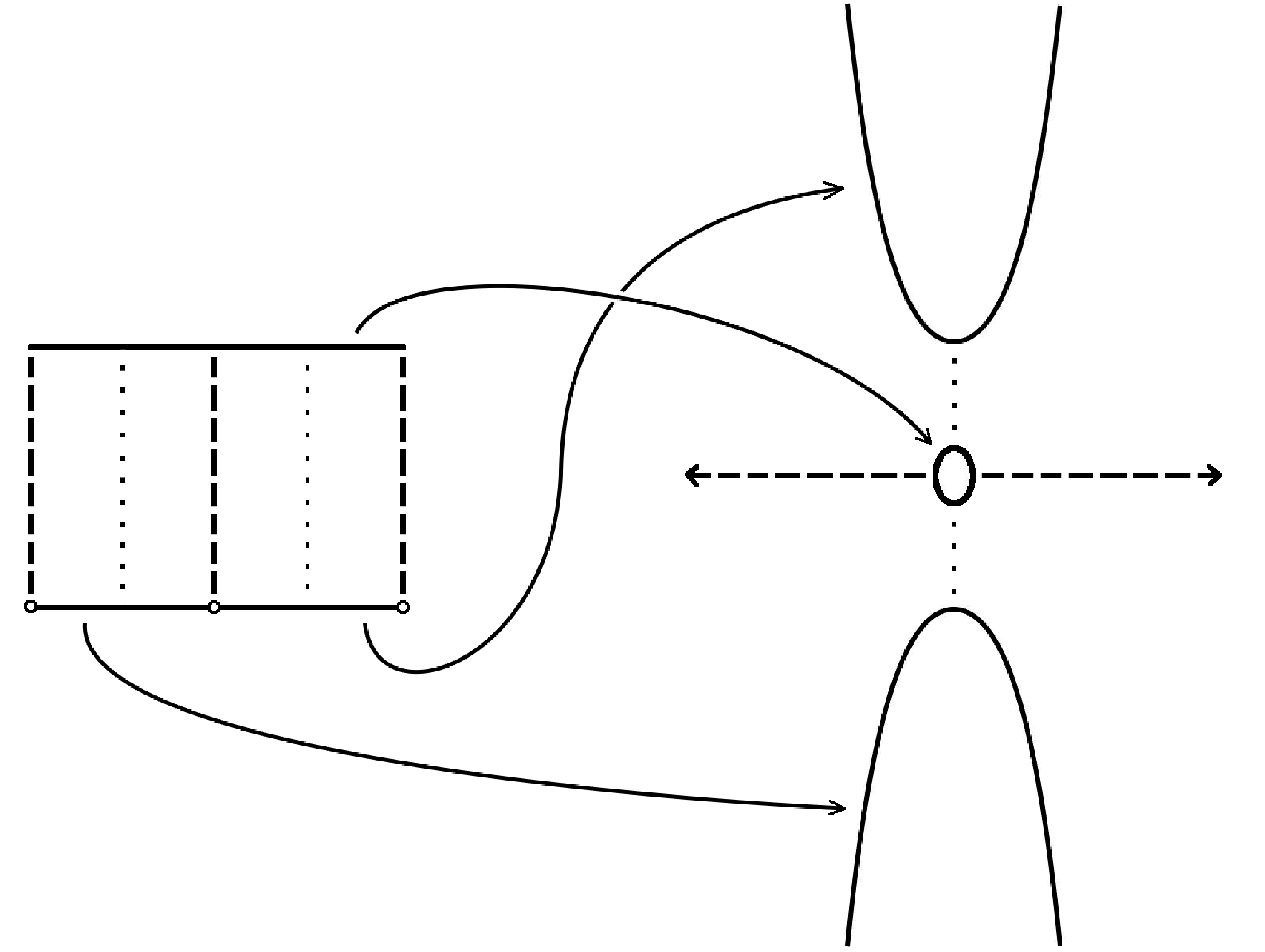
In order to show that $f$ is in fact univalent, it is enough to show that it is one-to-one on the the horizontal sides of $G$ (since $f$ is locally univalent). To this end, we make the following claims:

Claim 1 implies that $\mathrm{Re}\,f$ is monotone along each of the named segments, and since $\mathrm{Im}\,f$ differs between the two segments by Claim 2, $f$ must be one-to-one on the top side of $G$. Claim 4 implies that $f$ is one-to-one on each of the two segments on the bottom side of $G$. Claims 3, 5, and 6 imply that the images of these three segments do not intersect each other. This shows that $f$ is one-to-one on the horizontal sides of $G$.

The claims can be established by the properties of $f^{\prime}=F=\partial_{z}vB$. First note that, since $v(z)$ is positive in $G$ and vanishes on the horizontal sides of $G$, we have $\partial_{x}v(z)=0$ on both sides, and for $x\in{\mathbb{R}}$ we have $\partial_{y}v(x+\omega_{3})<0$, and $\partial_{y}v(x)>0$. In particular, $i\partial_{z}v(z)=i(\partial_{x}v-i\partial_{y}v)/2=\partial_{y}v/2$ is real. The function $B(z)$ is a Jacobi sn function, whose properties are well-known [2, Section 47]. $B(z)$ sends the top side of $G$ to the unit circle, such that the four segments $[\omega^{\prime},\omega^{\prime}+\omega]$, $[\omega^{\prime}+\omega,\omega^{\prime}+2\omega]$, $[\omega^{\prime}+2\omega,\omega^{\prime}+3\omega]$, and $[\omega^{\prime}+3\omega,\omega^{\prime}+4\omega]$ correspond to the fourth, third, second, and first quadrants of the unit circle, respectively. Multiplication by $\partial_{z}v(z)$ distorts this circle and rotates it by an angle of $\pi/2$ (since $\partial_{z}v(z)/i$ is positive) but preserves the two-fold symmetry. This determines the sign of the real and imaginary parts of $f^{\prime}$. Since $dz=dx$ is purely real on the horizontal sides of $G$, this gives the monotonicity of $\mathrm{Re}\,f$ stated in Claim 1. Claims 2 and 3 follow from the sign of $\mathrm{Im}\,f^{\prime}$ and the fact that $\mathrm{Im}\,f^{\prime}$ is an odd function with respect to reflection in each of the points $\omega^{\prime}+\omega$ and $\omega^{\prime}+3\omega$.

The four segments $[0,\omega]$, $[\omega,2\omega]$, $[2\omega,3\omega]$, and $[3\omega,4\omega]$ on the bottom side of $G$ are sent to the second, first, fourth, and third quadrants of the unit circle respectively. Since $\partial_{z}v(z)/i$ is negative along the bottom side of $G$, under $f^{\prime}(z)$ this becomes the first, fourth, third, and second quadrants, respectively. This establishes Claim 4, and combined with the reflectional symmetry, also Claim 5. Claim 6 follows from the fact that $\partial_{z}v(z)B(z)>0$ along the vertical segment $[\omega,\omega+\omega^{\prime}]$ and $\partial_{z}v(z)B(z)<0$ along $[3\omega,3\omega+\omega^{\prime}]$.

Only small modifications of the previous example are needed. Using the same $G,G^{\prime}$, $\omega_{1},\omega_{3}$, we define $h$ as the $\omega_{1}$-periodic function, positive and harmonic in $G^{\prime}$ except two logarithmic poles at $i\epsilon$ and $\omega_{1}+i\epsilon$, where $\epsilon\in(0,\omega_{3}/2)$. Then we can find constants $c_{1}$ and $c_{2}$ such that $v=h+c_{1}y+c_{2}$ has critical points at $\omega_{1}/2+\omega_{3}/2$ and $3\omega_{1}/2+\omega_{3}/2$.

Then $v_{z}$ is an elliptic function with periods $\omega_{1}$, $2\omega_{3}$ with two simple poles at $i\epsilon$ and $-i\epsilon$ per period parallelogram. This elliptic function has the form

with some small real $c$. The rest of the construction is the same as in the previous example.

In a similar manner to the above, in order to plot the figures, we expressed $F$ as a ratio of Weierstrass $\sigma$ functions:

Let $G_{j}$ be smooth Jordan domains on the plane whose closures are disjoint, and

Let $F$ be a complex potential of a flow of an ideal fluid which is divergence-free and locally irrotational in $D$. If the pressure (determined by $|F^{\prime}|$ according to Bernoulli’s law) is constant on $\partial D$ then $G_{j}$ can be interpreted as constant-pressure gas bubbles in the flow.

The first examples of this situation, with two bubbles were constructed by Pocklington [14]. Periodic exceptional domains give periodic examples with one bubble per period, with the flow on the surface on the bubbles rotating in the same direction [3] (see also [6]). Crowdy and Green [6] constructed periodic examples with two bubbles per period rotating in the opposite direction. Our example of type II can be interpreted as a periodic flow with two bubbles per period rotating in the same direction.

The velocity at infinity in our examples is directed in the opposite directions on the two sides of the row of the bubbles.

Department of Mathematics, Purdue University, West Lafayette, IN 47907 USA

References

- [1] L. Ahlfors, Conformal invariants, McGraw Hill Co., NY, 1973.
- [2] N. I Akhiezer, Elements of the theory of elliptic functions, AMS, Providence, RI, 1990.
- [3] G. Baker, P. Saffman, J. Sheffield, Structure of a linear array of hollow vortices of finite cross-section, J. Fluid Mech, 74, 3 (1976) 469–476.
- [4] M. Brelot, On topologies and boundaries in potential theory, Springer 1971.
- [5] T. Carleman, Extension d’un théorm̀e de Liouville, Acta Math. 48 (1926) 363–366.
- [6] D. Crowdy, C. C. Green, Analytical solutions for von Kármán streets of hollow vortices, Phys. Fluids 23 (2011), 126602.
- [7] P. Duren, Theory of spaces, Dover Publications, 2000.
- [8] B. Gustafsson, Application of half-order differentials on Riemann surfaces to quadrature identities for arc-length, J. d’Analyse Math. 49 (1987), 54–89.
- [9] M. Heins, A lemma on positive harmonic functions, Ann. Math., 52 (1950), 568-573.
- [10] L. Hauswirth, F. Helen and F. Pacard, On an overdetermined elliptic problem, Pacific J. Math., 250 (2011), 319–334.
- [11] D. Khavinson, E. Lundberg, R. Teodorescu, An overdetermined problem in potential theory, Pacific J. Math., 265 (2013), 85-111.
- [12] B. Kjellberg, On the growth of minimal positive harmonic functions in a plane region, Ark. Mat. 1 (1950), 347-351.
- [13] M. Longuet-Higgins, Limiting forms of capillary-gravity waves, J. Fluid Mech., 194 (1988) 351–357.
- [14] H. C. Pocklington, The configuration of a pair of equal and opposite hollow straight vortices of finite cross-section, moving steadily through fluid, Proc. Cambridge Phi. Soc., 8, 178 (1895).
- [15] Ch. Pommerenke, Univalent Functions, Vandenhoeck and Ruprecht, Göttingen, 1975.
- [16] A. Rashkovskii, Classical and new loglog theorems, Expo. Math., 27 (2009) 271–287.
- [17] M. Sakai, Null quadrature domains, Journal d’Analyse Math., 40 (1981), 144-154.
- [18] M. Traizet, Classification of the solutions to an overdetermined problem in the plane, Geometric and Functional Analysis, 24 (2014), 690-720.