Mixed Tempered Stable distribution
Abstract
In this paper we introduce a new parametric distribution, the Mixed Tempered Stable. It has the same structure of the Normal Variance Mean Mixtures but the normality assumption leaves place to a semi-heavy tailed distribution. We show that, by choosing appropriately the parameters of the distribution and under the concrete specification of the mixing random variable, it is possible to obtain some well-known distributions as special cases.
We employ the Mixed Tempered Stable distribution which has many attractive features for modeling univariate returns. Our results suggest that it is enough flexible to accomodate different density shapes. Furthermore, the analysis applied to statistical time series shows that our approach provides a better fit than competing distributions that are common in the practice of finance.
Keywords: Tempered Stable distribution; Mixture Models; Statistical Factors; Independent Component Analysis; Gamma density;
1 Introduction
The Stable distribution has gained a great popularity in modeling economic and financial time series starting from the seminal work of [23]. However, empirical evidence is against using the normal distibution for daily data but cannot accomodate the heavy tailedness of the Stable distribution. From a mathematical point of view a drawback of the Stable distribution is that only fractional moments of order with exist and, consequently, the standard Central Limit Theorem does not hold. For this reason, several researchers have considered the Tempered Stable distribution [8] as a valid alternative in modeling financial returns.
The Tempered Stable distribution can be obtained by multiplying the Lévy density of an - Stable with a decreasing tempering function . The tail behavior changes from heavy to semi-heavy characterized by an exponential instead of a power decay. The existence of the conventional moments is ensured and it satisfies the conditions of the classical Central Limit Theorem. This is an advantage in asset return modeling since for monthly or annual data the normality assumption seems to be correct [see[7] for survey of the stylized facts].
In this paper we propose a new distribution: the Mixed Tempered Stable (MixedTS henceforth). The idea is to build a new distribution in a similar way of the Normal Variance Mean Mixture (NVMM see [1]) where the normality assumption is substituted with the standardized Tempered Stable (see [13]). We show that the new distribution can overcome some limits of the NVMM. In particular, the asymmetry and the kurtosis do not depend only on the mixing random variable but also on the other variable that determines the distribution.
If the mixing random variable follows a Gamma distribution, the proposed model can have the Variance Gamma [22, 20], the Tempered Stable [8] and the Geometric Stable [15] as special cases for specific choice of the parameters.
In order to understand how this distribution fits to real data, we consider two examples. In the first, we build a Garch(1,1) with MixedTS innovations and use it in modeling univariate financial time series. In the second, we consider a multifactor model for the log returns of a fund which tries to replicate the performance of the S&P 500 index. As factors, we consider the Global Industry Classification Standard (GICS) indexes developed by MSCI-Barra provider. We capture the GICS dependence structure using the Independent Component Analysis introduced by [6] and developed by [10].
Once fixed the number of the Independent Components (ICs), we use the Mixed Tempered Stable to model each of them. The observed fund returns are the sum of the ICs and the single factor return density could be non-gaussian and/or semi-heavy tailed.
The Independent Component Analysis has been already used in finance and in particular to model interest rates term structures [2]. [21] proposed a non-Gaussian factor model using ICA with components assumed to follow a Variance Gamma distribution. Our model can be seen as a generalization of the latter since the Variance Gamma is a particular case of the Mixed Tempered Stable distribution. Following the same approach as in [24] and [25], the marginal contribution to risk of each factor can be easily computed for given homogeneous risk measures due to the independence assumption for the components.
The outline of the paper is as follows. In Section 2 we review the main characteristics of the Tempered Stable distribution and make some useful observations . In Section 3 we introduce the Mixed Tempered Stable distribution and its main features. Section 4 illustrates the fitting of the MixedTS distribution to financial time series and to the Independent Components. Section 5 concludes the paper.
2 Tempered Stable distribution
In this section we review the main features of the Tempered Stable distribution. A random variable follows a Tempered Stable distribution if its Lévy measure is given by:
| (1) |
with and .
The characteristic function is obtained by solving the integral [8]:
where . As observed in [19], for , the Tempered Stable is obtained as a difference of two independent one sided Tempered Stable distributions introduced in [27]. The corresponding process has finite variation with infinite activity. The interest of researchers for this distribution is confirmed from the fact that many particular cases have been investigated in literature. For and , we get the CGMY distribution [4]. If we fix and , we get the truncated Lévy flight introduced in [14] while for we get the Bilateral Gamma distribution [16, 17, 18]. Computing the limit for , and we obtain the Variance Gamma distribution [see[22, 20] for estimation]. In this paper, we consider the same restrictions as in [13], i.e : and where the distribution of the r.v is called Classical Tempered Stable. For this r.v and its characteristic function is given by:
The cumulant of order n for the r.v X can be obtained by taking the derivative of the characteristic exponent:
| (3) |
Given the parameters of the distribution and fixing , we get:
| (4) |
and for :
| (5) |
Using the cumulants we get the first four moments of the distribution:
| (6) |
From the skewness formula it can be noticed that the difference between and drives the asymmetry while for the sign of the skewness depends on the difference of the two tempering parameters and .
The following result shows the convergence of the Tempered Stable distribution to the symmetric Stable distribution.
Proposition 1
For , and , the Tempered Stable distribution converges to the symmetric Stable distribution when goes to zero.
For , and , the characteristic exponent in () becomes the characteristic function of a symmetric Tempered Stable distribution:
| (7) |
For and :
where the last equality is due to the Euler equation . The limit for gives a more compact formula for the characteristic function:
| (8) |
that in fact is the characteristic function of a symmetric Stable distribution.
Remark 2
The r.v has zero mean and unit variance for and
| (9) |
The distibution of the r.v X is called standardized Classical Tempered Stable, i.e .
It is useful to observe that in the standardized Classical Tempered Stable distribution is fully determined once given the values for , and . Its characteristic exponent, defined as , is:
| (10) |
For , we get the characteristic exponent of the Normal distribution :
Remark 3
Condition (9) implies that the convergence to stable is not possible since the characteristic exponent would converge to zero.
If the tempering parameters depend on a strictly positive quantity h, the standardized Classical Tempered Stable distribution has the following property that makes it appealing for mixtures.
Proposition 4
Let and then the random variable has the following characteristic exponent:
| (11) |
Moreover if we have:
| (12) |
where are iid
Proof. The characteristic exponent (10) evaluated in gives:
Factorize :
and through simple manipulations we obtain the result in (11).
To prove the result in equation (12) we use the iid assumption for , where . The characteristic exponent of the random variable becomes:
where . Using equation (10) we obtain the characteristic exponent of that implies the relation in equation (12).
3 Mixed Tempered Stable distribution
In this section, using proposition 4, we define a new distribution that is shown to have some nice mathematical and statistical features.
Definition 5
We say that a continuous random variable Y follows a Mixed Tempered Stable distribution if:
| (13) |
where . V is a Lévy distribution defined on the positive axis and its moment generating function (mgf) always exists.
The logarithm of the mgf is :
| (14) |
We apply the law of iterated expectation for the computation of the characteristic function for the new distribution :
The characteristic function identifies the distribution at time one of a time changed Lévy process that as shown in [26] and [5] it is infinitely divisible.
Proposition 6
The first four moments for the MixedTS are:
In Figure 1 we show the behaviour of the skewness for different combinations of and and fixed . The same is done in Figure 2 for the kurtosis.
Insert here Figure 1.
Insert here Figure 2.
If we assume that , the characteristic exponent in () becomes:
Using the scaling property for the Gamma distribution (see [11]), the r.v. can be equivalently defined as:
| (17) |
where and .
The MixedTS with Gamma mixing density has as special cases some well known distributions widely applied in different fields. Indeed, for and computing the limit for going to infinity, we retrieve the standardized Classical Tempered Stable (see Figure 3(b)). The symmetric Variance Gamma distribution is obtained by choosing as shown in Figure 3(a). By choosing:
and computing the limit for we obtain the Geometric Stable distribution. Substituting the conditions () in the characteristic exponent definition, we have:
Applying the limit and following the same arguments of proposition 1, we get:
for any . The convergence to the Geometric-Stable distribution is shown in Figure 3(c).
Insert Figure 3 here.
The comparison of the MixedTS with the asymmetric Variance Gamma distribution, requires a more general version of equation 17. In practice, we consider a new random variable as follows:
| (19) |
where is defined in equation 17. In this way, we can have the mean to be different from zero and a model that is easier to be compared with the NVMM since the structure is the same.
4 Empirical study
In this section we empirically investigate the performance of the MixedTS distribution in modeling asset returns by considering two examples. In the first, we study the ability of the new model to capture the stylized facts observed in each asset return time series. We use the MixedTS for the innovations of a Garch(1,1) and compare its performance with a Garch(1,1) with Variance Gamma innovations.
In the second, we build a multifactor model using the Independent Component Analysis and assume that each component follows a MixedTS distribution with Gamma mixing density.
The dataset is composed by daily log returns of the Vanguard Fund Index which tries to replicate the performance of the S&P 500. It seems quite natural to consider as portfolio risk factors the daily log-returns of the 10 GICS indexes since each of the S&P500 members belongs to one of them. The data are daily log returns ranging from 14-June-2010 to 20-September-2012 obtained from the Bloomberg data provider.
In Table 1 we report the main statistics of the considered indexes. Looking to the empirical skewness and kurtosis, the departure from the normal hypothesis is evident.
Insert Table 1 here.
In the first example, log returns are modeled using the classical Garch(1,1) as in [3] :
| (20) | |||||
| (21) |
where follows the general MixedTS defined in equation 19. The model is compared with another Garch(1,1) with the same structure but is Variance Gamma distributed. Using the quasi-maximum likelihood method [3], implemented in the Garch Matlab toolbox, we get the values for the parameters and the volatility sequence for . We estimate the values for the MixedTS parameters on the residual sequence minimizing the mean squared error computed using the empirical and the theoretical densities. In the MixedTS case, the density is computed using the Fourier transform while for the Variance Gamma we apply the approximation proposed in [20]. As measures of fit we consider the Mortara index , the quadratic Pearson index and the root of mean squared errors :
where we consider classes for the observations, are the observed frequencies and the theoretical frequencies for the classes.
The estimated parameters for the Vanguard Fund Index and GICS are reported in Table 3.
Insert Table 3 here.
Values for lower than two suggest that the empirical distribution cannot be modeled considering only the Variance Gamma. The better fit of the MixedTS with respect to the Variance Gamma is confirmed by comparing the fitting measures in Table 3.
In the second example, we assume a linear relation of the Vanguard Fund returns with the ten risk factors built using daily log returns of the GICS indexes :
| (23) |
where and contain respectively the log returns of the Vanguard Fund and of the i-th sector. In we put the exposure of the portfolio returns to the i-th factor while is the idiosyncratic noise term. Through a simple Ordinary Least Squares regression, we get the exposures to the risk factors whose results are reported in Table 2. In particular, we observe that the is higher than suggesting that the considered risk factors explain almost all the variability present in the Vanguard Fund log returns. Moreover, looking at Table 2, we observe that the estimated factor exposures in are coherent with the market capitalization of each sector.
Insert Table 2 here.
We apply the FastICA algorithm proposed by [9] to the GICS and find the Independent Components (ICs) that maximize the non-gaussianity condition present in the optimization algorithm. If we think to the ICs as the columns of a matrix , the ten sectors time series can be seen as linear transformations of the independent signal sources. In the mixing matrix is contained the information about the weight of the single original source in the market sector, i.e . The methodology is closely related to the well known Principal Component Analysis (see [12]). However, while in the latter we assume that the unknown factors are normally distributed, in the ICA analysis factors are identified by maximizing any measure of non-Gaussianity for each component. Portfolio return distribution is obtained as a linear combination of independent r.v’s that can have different distributions. We use the Jarque-Bera test to check for non-normality even though the departure from normality is confirmed even by sample skewness and kurtosis reported in Table 4.
Insert here Table 4.
In matrix notations, portfolio return can be decomposed in the form:
| (24) |
with being the matrix containing the rows of the matrix containing the components we decide to be meaningful in the market and with the remaining components considered as noise. The new exposures and are obtained by multiplying of the initial exposures with the corresponding vectors in the mixing matrix .
The linear relation in the portfolio return model can be used to compute the marginal contribution to return/risk of each of the chosen IC (as done in [24] or in [25]) or in a portfolio optimization problem as in [21]. We emphasize the fact that our main focus is not on introducing a new method on how to use ICA in finance but to stress the flexibility of the Mixed Tempered Stable distribution that can allow to capture contemporaneously the different shapes of each IC. In Table 5 we report the estimated mixing matrix obtained using the FastICA algorithm and observe that the MixedTS can fit statistical time series having different shapes.
Insert here table 5.
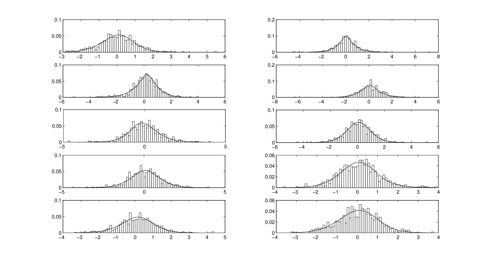
The empirical densities of the independent components are shown in Figure 4. In Table 6 we give the MixedTS fitted parameters for each component and some measures of fit.
Insert here Figure 4.
Insert here Table 6.
The four ICs with the highest Jarque Bera statistic are considered as factors while the others are grouped in the noise term . The independence of and simplifies the computations since we are able to compute the characteristic function for the portfolio returns :
The Vanguard return density is reconstructed using the calibrated MixedTS distribution parameters for the factors and assuming normality for the noise. It is possible to recover the density of the r.v from its characteristic function using the Fourier Transform. For comparison, we plot the normal distribution fitted to the fund return density.5
Insert here Figure 5
5 Conclusion
In this article, we discussed various features of the Tempered Stable distribution and introduced a new parametric distribution named Mixed Tempered Stable. The existing Normal Variance Mean Mixture models are based on the normality assumption while we try to generalize this concept. In fact, we consider the Standardized Classical Tempered Stable instead of the Gaussian distribution. The mixing r.v is defined on the positive axis but we showed that if it is Gamma distributed the Variance Gamma, the Tempered Stable and the Geometric Stable distribution are special cases. Despite the fact that this distribution has nice features from a theoretical point of view, it allows a dependence of the standard higher moments not only on the mixing r.v but also on the Standardized Classical Tempered Stable distribution. As part of our investigation, we also perform a sensitivity analysis of the skewness and kurtosis on the model parameters.
As a first step, in our empirical study, we model the univariate financial returns using a Garch(1,1) with MixedTS innovations and compare the results in terms of fitting with the same model but with Variance Gamma innovations.
Finally, we investigate the fitting of the MixedTS distribution to the time series of the statistical factors obtained by applying the FastICA algorithm on the ten GICS sectors. It is important to have a flexible distribution for accomodating the differences in terms of asymmetry and tail heaviness in the ICs. The fitting measures involved in the analysis confirm the theoretical findings and justify the superior performance of our model.
References
- [1] O.E. Barndorff-Nielsen, J. Kent, and M. Sørensen. Normal variance-mean mixtures and z-distributions. International Statistical Review, 50:145–159, 1982.
- [2] F Bellini and E Salinelli. Independent component analysis and immunization: an exploratory study. International Journal of theoretical and applied finance, 6(7):721 – 738, 2003.
- [3] T Bollerslev. A conditionally heteroskedastic time series model for speculative prices and rates of return. The Review of Economics and Statistics, 69(3):542–547, 1987.
- [4] P. Carr, H. Geman, D.B. Madan, and M. Yor. The fine structure of asset returns: an empirical investigation. Journal of Business, 75(2):305–332, 2002.
- [5] P. Carr and L. Wu. Time-changed levy processes and option pricing. Journal of Financial Economics, 71(1):113–141, 2004.
- [6] P. Comon. Independent component analysis, a new concept? Signal Process., 36(3):287–314, 1994.
- [7] R. Cont. Empirical properties of asset returns: stylized facts and statistical issues. Quantitative Finance, 1:223–236, 2001.
- [8] R. Cont and P. Tankov. Financial Modelling with Jump Processes, volume II. Chapman & Hall/CRC Financial Mathematics Series, New York, 2003.
- [9] A. Hyvärinen. Fast and robust fixed-point algorithms for independent component analysis. IEEE Transactions on Neural Networks, 10(3):626–634, 1999.
- [10] A. Hyvärinen and E. Oja. Independent Component Analysis. New York: Wiley, 2001.
- [11] N.L. Johnson, S. Kotz, and N. Balakrishnan. Continuous Univariate Distributions, volume I. Wiley Series in Probability and Statistics, 2002.
- [12] I.T. Jolliffe. Principal Component Analysis, volume II of 68. Springer, second edition, 2002.
- [13] Y.S. Kim, S. T. Rachev, M. L. Bianchi, and F.J. Fabozzi. Financial market models with lévy processes and time-varying volatility. Journal of Banking and Finance, 32(7):1363–1378, 2008.
- [14] I. Koponen. Analytic approach to the problem of convergence of truncated lévy flights towards the gaussian stochastic process. Physical Review E, 52:1197–1199, 1995.
- [15] T. J. Kozubowski, K. Podgórski, and G. Samorodnitsky. Tails of lévy measure of geometric stable random variables, 1997.
- [16] U. Küchler and S. Tappe. Bilateral gamma distributions and processes in financial mathematics. Stochastic Processes and their Applications, 118(2):261–283, 2008.
- [17] U. Küchler and S. Tappe. On the shapes of bilateral gamma densities. Statistics and Probability Letters, 78(15):2478–2484, 2008.
- [18] U. Küchler and S. Tappe. Option pricing in bilateral gamma stock models. Statistics and Decisions, 27:281–307, 2009.
- [19] U. Küchler and S. Tappe. Tempered stable distributions and processes. Stochastic Processes and their Applications, 2013.
- [20] A. Loregian, L. Mercuri, and E. Rroji. Approximation of the variance gamma model with a finite mixture of normals. Statistic & Probability Letters, 82(2):217–224, 2012.
- [21] D. B. Madan. Equilibrium asset pricing: with non-gaussian factors and exponential utilities. Quantitative Finance, 6(6):455–463, 2006.
- [22] D.B. Madan and B. Seneta. The vg model for share market returns. Journal of Business, 63:511–524, 1990.
- [23] B. B. Mandelbrot. The variation of certain speculative prices. The Journal of Business, 36, 1963.
- [24] A. Meucci. Risk and Asset Allocation. Springer, Berlin, 2005.
- [25] E. Rroji. Risk attribution and semi-heavy tailed distributions. Phd thesis, University of Milano-Bicocca, 2013.
- [26] K. I. Sato. Lévy Processes and Infinitely Divisible Distributions, volume II of 68. Cambridge studies in advanced mathematics, 1998.
- [27] M. Tweedie. An index whichg distinguishes between some important exponantial families. In Proc. Indian Statistical Institute Golden Jubilee International Conference,, pages 579–604. J. Ghosh and J. Roy (Eds.), 1984.


| Mean | Std | Skew | Ex-Kurt | Min | Max | |
|---|---|---|---|---|---|---|
| VFIAX | 0.0005 | 0.0121 | -0.4693 | 3.9683 | -0.0688 | 0.0463 |
| COND | 0.0007 | 0.0129 | -0.5674 | 3.0566 | -0.0690 | 0.0472 |
| CONS | 0.0006 | 0.0078 | -0.3871 | 3.2413 | -0.0390 | 0.0332 |
| ENRS | 0.0006 | 0.0158 | -0.3878 | 3.3909 | -0.0864 | 0.0687 |
| FINL | 0.0002 | 0.0175 | -0.3415 | 4.1493 | -0.1052 | 0.0789 |
| HLTH | 0.0006 | 0.0101 | -0.4205 | 3.9130 | -0.0540 | 0.0456 |
| INDU | 0.0004 | 0.0142 | -0.4390 | 2.7993 | -0.0711 | 0.0495 |
| INFT | 0.0007 | 0.0130 | -0.2948 | 2.0849 | -0.0596 | 0.0445 |
| MATR | 0.0005 | 0.0159 | -0.3575 | 2.5824 | -0.0756 | 0.0593 |
| TELS | 0.0007 | 0.0097 | -0.2897 | 2.9581 | -0.0550 | 0.0426 |
| UTIL | 0.0004 | 0.0089 | -0.1124 | 4.7863 | -0.0563 | 0.0414 |
| Regression coefficients and Capitalization weights | ||||||||||
| COND | CONS | ENRS | FINL | HLTH | INDU | INFT | MATR | TELS | UTIL | |
| 0.1105 | 0.1154 | 0.1238 | 0.1442 | 0.1051 | 0.1145 | 0.1818 | 0.0378 | 0.0220 | 0.0415 | |
| Cap weight (14/06/2010) | 0.1103 | 0.1165 | 0.1206 | 0.1441 | 0.1190 | 0.1221 | 0.1800 | 0.0115 | 0.0213 | 0.0546 |
| Cap weight (20/09/2012) | 0.1108 | 0.1091 | 0.1127 | 0.1507 | 0.1228 | 0.099 | 0.1921 | 0.0349 | 0.0317 | 0.0362 |
| VFIAX | COND | CONS | ENRS | FINL | HLTH | INDU | INFT | MATR | TELS | UTIL | |
|---|---|---|---|---|---|---|---|---|---|---|---|
| -0.0681 | -0.0318 | 0.1399 | -0.3049 | -0.0830 | -0.0338 | -0.0655 | 0.0064 | -0.0212 | 0.6256 | 0.0936 | |
| 0.0601 | 0.0227 | -0.0454 | 0.1310 | 0.0204 | 0.0780 | 0.0232 | -0.0311 | 0.0605 | -0.1931 | -0.0409 | |
| 1.0530 | 0.7276 | 0.5038 | 0.8314 | 0.7026 | 1.1109 | 0.7843 | 0.8554 | 1.0803 | 0.5487 | 0.5291 | |
| a | 1.1670 | 2.0313 | 3.8303 | 1.9440 | 2.2742 | 0.9718 | 1.8799 | 1.5514 | 1.2326 | 3.2875 | 3.4667 |
| 1.0280 | 1.0384 | 1.0855 | 1.6044 | 1.0921 | 1.0000 | 1.0635 | 1.0540 | 0.9942 | 0.4083 | 0.9824 | |
| 1.0311 | 1.0786 | 1.1733 | 0.4052 | 1.0961 | 1.0000 | 1.0801 | 1.0925 | 1.6001 | 1.9144 | 1.2202 | |
| 1.4717 | 1.6663 | 1.9189 | 1.2897 | 1.7461 | 1.3000 | 1.6610 | 1.5913 | 1.3256 | 1.5053 | 1.8437 | |
| A_2_MixedTS | 0.0060 | 0.0055 | 0.0035 | 0.0065 | 0.0047 | 0.0055 | 0.0048 | 0.0046 | 0.0057 | 0.0061 | 0.0093 |
| X_2_MixedTS | 0.0400 | 0.0333 | 0.0345 | 0.0413 | 0.0365 | 0.0317 | 0.0363 | 0.0370 | 0.0393 | 0.0363 | 0.0474 |
| A_1_MixedTS | 0.0038 | 0.0036 | 0.0021 | 0.0042 | 0.0034 | 0.0037 | 0.0037 | 0.0038 | 0.0039 | 0.0034 | 0.0061 |
| A_2_VG | 0.0062 | 0.0066 | 0.0066 | 0.0071 | 0.0057 | 0.0092 | 0.0058 | 0.0048 | 0.0063 | 0.0075 | 0.0069 |
| X_2_VG | 0.0449 | 0.0346 | 0.0384 | 0.0435 | 0.0377 | 0.0345 | 0.0383 | 0.037 | 0.0385 | 0.0415 | 0.0555 |
| A_1_VG | 0.0042 | 0.0040 | 0.0041 | 0.00500 | 0.0042 | 0.0055 | 0.0044 | 0.0039 | 0.0042 | 0.0042 | 0.0047 |
| Statistics ICs | ||||||||||
|---|---|---|---|---|---|---|---|---|---|---|
| I | II | III | IV | V | VI | VII | VIII | IX | X | |
| Skewness | -0.6496 | -0.1200 | -0.5531 | 0.2913 | -0.0349 | -0.2916 | 0.0876 | -0.1975 | -0.0881 | -0.0021 |
| Kurtosis | 7.7030 | 7.5633 | 5.9752 | 5.9352 | 4.6628 | 4.1283 | 4.2410 | 3.7250 | 3.6370 | 3.4420 |
| JB-Statistic | 546.5730 | 479.4040 | 231.3230 | 205.6020 | 63.5910 | 37.0450 | 36.0660 | 15.6540 | 10.0440 | 4.4830 |
| Mixing Matrix | |||||||||
|---|---|---|---|---|---|---|---|---|---|
| I | II | III | IV | V | VI | VII | VIII | IX | X |
| -0.0035 | -0.0098 | -0.0016 | 0.0024 | -0.0018 | 0.0035 | -0.0044 | -0.0014 | 0.0028 | 0.0023 |
| -0.0008 | -0.0059 | -0.0001 | 0.0030 | -0.0007 | 0.0029 | 0.0002 | -0.0006 | 0.0021 | -0.0014 |
| 0.0030 | -0.0126 | -0.0006 | 0.0013 | 0.0000 | 0.0029 | -0.0067 | -0.0034 | 0.0034 | -0.0015 |
| -0.0022 | -0.0149 | -0.0020 | 0.0047 | 0.0023 | 0.0030 | -0.0052 | -0.0027 | -0.0027 | 0.0005 |
| -0.0021 | -0.0083 | -0.0017 | 0.0029 | -0.0005 | 0.0002 | -0.0026 | 0.0005 | 0.0027 | -0.0020 |
| -0.0036 | -0.0103 | -0.0016 | 0.0029 | 0.0018 | 0.0035 | -0.0055 | -0.0037 | 0.0031 | -0.0009 |
| -0.0028 | -0.0089 | -0.0030 | 0.0027 | -0.0038 | 0.0019 | -0.0046 | -0.0050 | 0.0015 | -0.0008 |
| -0.0019 | -0.0113 | -0.0023 | 0.0005 | -0.0003 | 0.0060 | -0.0082 | -0.0018 | 0.0013 | -0.0028 |
| -0.0029 | -0.0077 | 0.0044 | 0.0013 | -0.0010 | 0.0006 | -0.0012 | -0.0011 | 0.0007 | -0.0017 |
| -0.0012 | -0.0080 | -0.0009 | -0.0008 | 0.0004 | 0.0014 | 0.0018 | -0.0011 | 0.0018 | -0.0011 |
| MixedTS Parameters and Fitting Measures | ||||||||||
| I | II | III | IV | V | VI | VII | VIII | IX | X | |
| -0.0771 | 0.1951 | -0.1085 | 0.2336 | 0.5330 | -0.6738 | -0.4341 | -1.5481 | -5.1370 | 0.2181 | |
| 0.0275 | -0.0915 | 0.0487 | -0.1786 | -0.3415 | 0.2133 | 0.1610 | 0.1025 | 0.1646 | -0.0858 | |
| 1.0146 | 0.6666 | 0.7919 | 0.7814 | 0.8071 | 0.5983 | 0.6371 | 0.2595 | 0.1907 | 0.6358 | |
| 1.2686 | 2.3377 | 2.1517 | 2.0305 | 1.4409 | 3.2953 | 2.8364 | 14.7360 | 30.4567 | 2.5446 | |
| 1.0247 | 0.9146 | 1.8861 | 1.0256 | 1.0000 | 1.8062 | 2.2127 | 8.2816 | 9.9490 | 1.0890 | |
| 0.9965 | 1.3665 | 0.1000 | 1.0431 | 1.0000 | 0.1000 | 0.6080 | 0.1000 | 0.1000 | 1.2074 | |
| 1.3724 | 1.7579 | 1.7150 | 1.5458 | 1.3000 | 1.6660 | 1.5057 | 1.7187 | 0.5000 | 1.8469 | |
| 0.0082 | 0.0064 | 0.0059 | 0.0072 | 0.0076 | 0.0036 | 0.0077 | 0.0062 | 0.0052 | 0.0063 | |
| 0.0463 | 0.0781 | 0.0471 | 0.0512 | 0.0439 | 0.0314 | 0.0482 | 0.0434 | 0.0314 | 0.0412 | |
| 0.0048 | 0.0040 | 0.0038 | 0.0052 | 0.0045 | 0.0026 | 0.0047 | 0.0043 | 0.0037 | 0.0038 | |
