跳到论文正文
W Papers独立论文阅读器 arXiv:1405.7357 论文正文 计算阅读时间 · 0%
引用这篇论文根据当前论文元数据生成,正式投稿前建议核对。


License: arXiv.org perpetual non-exclusive license
arXiv:1405.7357v2 [cond-mat.str-el] 23 Mar 2015

Quasi-Local Strange Metal

Shouvik Sur1 and Sung-Sik Lee1,2
1Department of Physics &\& Astronomy, McMaster University,
1280 Main St. W., Hamilton ON L8S 4M1, Canada
2Perimeter Institute for Theoretical Physics,
31 Caroline St. N., Waterloo ON N2L 2Y5, Canada
August 24, 2026
Abstract

One of the key factors that determine the fates of quantum many-body systems in the zero temperature limit is the competition between kinetic energy that delocalizes particles in space and interaction that promotes localization. While one dominates over the other in conventional metals and insulators, exotic states can arise at quantum critical points where none of them clearly wins. Here we present a novel metallic state that emerges at an antiferromagnetic (AF) quantum critical point in the presence of one-dimensional Fermi surfaces embedded in space dimensions three and below. At the critical point, interactions between particles are screened to zero in the low energy limit at the same time the kinetic energy is suppressed in certain spatial directions to the leading order in a perturbative expansion that becomes asymptotically exact in three dimensions. The resulting dispersionless and interactionless state exhibits distinct quasi-local strange metallic behaviors due to a subtle dynamical balance between screening and infrared singularity caused by spontaneous reduction of effective dimensionality. The strange metal, which is stable near three dimensions, shows enhanced fluctuations of bond density waves, d-wave pairing, and pair density waves.

The richness of exotic zero-temperature states in condensed matter systems[1, 2] can be attributed to quantum fluctuations driven by kinetic energy and interaction which can not be simultaneously minimized due to the uncertainty principle. In conventional metals, kinetic energy plays the dominant role, and interactions only dress electrons into quasiparticles which survive as coherent excitations in the absence of instabilities[3, 4]. The existence of well defined quasiparticle excitations is the cornerstone of Landau Fermi liquid theory[5], which successfully explains a large class of metals. However, the Fermi liquid theory breaks down at the verge of spontaneous formation of order in metals[6, 7, 8]. Near continuous quantum phase transitions, new metallic states can arise as quantum fluctuations of order parameter destroy the coherence of quasiparticles through interactions that persist down to the zero energy limit[9, 10]. Systematic understanding of the resulting strange metallic states is still lacking, although there exist some examples whose universal behaviors in the low energy limit can be understood within controlled theoretical frameworks[11, 12, 13, 14, 15].

Antiferromagnetic (AF) quantum phase transition commonly arises in strongly correlated systems including electron doped cuprates[16], iron pnictides[17] and heavy fermion compounds[18]. In two space dimensions, it has been shown that the interaction between the AF mode and itinerant electrons qualitatively modify the dynamics of the system at the critical point[19, 20]. A recent numerical simulation shows a strong enhancement of superconducting correlations near the AF critical point[21]. However, the precise nature of the putative strange metallic state has not been understood yet due to a lack of theoretical control over the strongly coupled theory that governs the critical point[22].

In this article, based on a controlled expansion, we show that a novel quantum state arises at the AF quantum critical point in metals that support one-dimensional Fermi surface through a non-trivial interplay between kinetic energy and interactions. To the lowest order in the perturbative expansion that becomes asymptotically exact at low energies in three dimensions, we find that quasiparticles are destroyed even though the interaction between electrons and the AF mode is screened to zero in the low energy limit. This unusual behavior is possible as the system develops an infinite sensitivity to the interaction through the kinetic energies that become dispersionless in certain spatial directions. The dynamical balance between vanishing kinetic energy and interactions results in a stable quasi-local strange metal which supports incoherent single-particle excitations and enhanced correlations for various competing orders.

Refer to caption
Figure 1: A two-dimensional Fermi surface where the shaded (unshaded) region represents occupied (unoccupied) states in momentum space. The hot spots on the Fermi surface are denoted as (red) dots. The (green) arrows represent the AF wavevector Q→A​F\vec{Q}_{AF}.

Model and dimensional regularization. We first consider two space dimensions. Although the specific lattice is not crucial for the following discussion, we consider the square lattice with the nearest and next-nearest neighbor hoppings. For electron density close to half-filling (one electron per site), the system supports a Fermi surface shown in Fig. 1. The minimal theory that describes the AF critical point in the two dimensional metal includes the collective AF fluctuations that are coupled to electrons near the hot spots, which are the set of points on the Fermi surface connected by the AF wavevector [19, 20, 22]. In this paper we consider the collinear AF order with a commensurate wavevector that is denoted as arrows in Fig. 1. If the AF order is incommensurate or non-collinear, the critical theory is modified from the one for the collinear AF order with a commensurate wavevector. As will be shown later, the simplest case we consider here already has quite intricate structures.

The action for the commensurate AF mode and the electrons near the hot spots reads

𝒮\displaystyle\mathcal{S} =∑n=14∑m=±∑σ=↑,↓∫d3​k(2​π)3ψn,σ(m)∗(k)[ik0+enm(k→)]ψn,σ(m)(k)\displaystyle=\sum_{n=1}^{4}\sum_{m=\pm}\sum_{\sigma=\uparrow,\downarrow}\int\frac{d^{3}k}{(2\pi)^{3}}~{\psi}^{(m)*}_{n,\sigma}(k)\left[ik_{0}~+e^{m}_{n}(\vec{k})\right]\psi^{(m)}_{n,\sigma}(k)
+12∫d3​q(2​π)3[q02+c2|q→|2]ϕ→(−q)⋅ϕ→(q)\displaystyle\quad+\frac{1}{2}\int\frac{d^{3}q}{(2\pi)^{3}}\left[q_{0}^{2}+c^{2}|\vec{q}|^{2}\right]\vec{\phi}(-q)\cdot\vec{\phi}(q)
+g0∑n=14∑σ,σ′=↑,↓∫d3​k(2​π)3d3​q(2​π)3[ϕ→(q)⋅ψn,σ(+)∗(k+q)τ→σ,σ′ψn,σ′(−)(k)+c.c.]\displaystyle\quad+g_{0}\sum_{n=1}^{4}\sum_{\sigma,\sigma^{\prime}=\uparrow,\downarrow}\int\frac{d^{3}k}{(2\pi)^{3}}\frac{d^{3}q}{(2\pi)^{3}}~\Bigl[\vec{\phi}(q)\cdot{\psi}^{(+)*}_{n,\sigma}(k+q)\vec{\tau}_{\sigma,\sigma^{\prime}}\psi^{(-)}_{n,\sigma^{\prime}}(k)+c.c.\Bigr]
+u04!∫d3​k1(2​π)3d3​k2(2​π)3d3​q(2​π)3[ϕ→(k1+q)⋅ϕ→(k2−q)][ϕ→(k1)⋅ϕ→(k2)].\displaystyle\quad+\frac{u_{0}}{4!}\int\frac{d^{3}k_{1}}{(2\pi)^{3}}\frac{d^{3}k_{2}}{(2\pi)^{3}}\frac{d^{3}q}{(2\pi)^{3}}\left[\vec{\phi}(k_{1}+q)\cdot\vec{\phi}(k_{2}-q)\right]\left[\vec{\phi}(k_{1})\cdot\vec{\phi}(k_{2})\right]. (1)

Here k=(k0,k→)k=(k_{0},\vec{k}) denotes frequency and two-dimensional momentum k→=(kx,ky)\vec{k}=(k_{x},k_{y}). ψn,σ(±)\psi^{(\pm)}_{n,\sigma}’s are fermionic fields which represent electrons of spin σ=↑,↓\sigma=\uparrow,\downarrow near the hot spots labeled by n=1,2,3,4n=1,2,3,4, m=±m=\pm, as is shown in Fig. 1. The axis in momentum space has been chosen such that the AF wavevector becomes Q→A​F=±2​π​y^=±2​π​x^{\vec{Q}}_{AF}=\pm\sqrt{2}\pi\hat{y}=\pm\sqrt{2}\pi\hat{x} up to the reciprocal vectors 2​π​(x^±y^)\sqrt{2}\pi(\hat{x}\pm\hat{y}). In this coordinate, the energy dispersions of the fermions near the hot spots can be written as e1±​(k→)=−e3±​(k→)=v​kx±kye_{1}^{\pm}(\vec{k})=-e_{3}^{\pm}(\vec{k})=vk_{x}\pm k_{y}, e2±​(k→)=−e4±​(k→)=∓kx+v​kye_{2}^{\pm}(\vec{k})=-e_{4}^{\pm}(\vec{k})=\mp k_{x}+vk_{y}, where k→\vec{k} represents deviation of momentum away from each hot spot. It is noted that local curvature of the Fermi surface can be ignored because the kk-linear terms dominate at low energies. The component of Fermi velocity parallel to Q→A​F{\vec{Q}}_{AF} at each hot spot is set to be unity up to sign by rescaling k→\vec{k}. vv measures the component of the Fermi velocity perpendicular to Q→A​F{\vec{Q}}_{AF}. If vv was zero, the hot spots connected by Q→A​F\vec{Q}_{AF} would be perfectly nested. ϕ→​(q)\vec{\phi}(q) represents three components of boson field which describes the fluctuating AF order parameter carrying frequency q0q_{0} and momentum Q→A​F+q→{\vec{Q}}_{AF}+\vec{q}. τ→\vec{\tau} represents the three generators of the S​U​(2)SU(2) group. cc is the velocity of the AF collective mode. g0g_{0} is the Yukawa coupling between the collective mode and the electrons near the hot spots, and u0u_{0} is the quartic coupling between the collective modes. v,c,g0,u0v,c,g_{0},u_{0} are genuine parameters of the theory, which can not be removed by redefinition of momentum or fields.

In two dimensions, the perturbative expansion in g0g_{0}, u0u_{0} fails because the couplings grow rapidly as the length scale is increased under the renormalization group (RG) flow. Although the growth of the couplings is tamed by screening, it is hard to follow the RG flow because the flow will stop (if it does) outside the perturbative window. In higher dimensions, the growth of the couplings becomes slower. Therefore we aim to tune the space dimension such that the balance between the slow growth of the couplings and the screening stabilizes the interacting theory at weak coupling. Here we increase the co-dimension of the Fermi surface while fixing its dimension to be one. A mere increase of co-dimension of the Fermi surface introduces a non-locality in the kinetic energy[23]. In order to keep locality of the theory, we introduce two-component spinors[14], by combining fermion fields on opposite sides of the Fermi surface, Ψ1,σ=(ψ1,σ(+),ψ3,σ(+))T\Psi_{1,\sigma}=(\psi^{(+)}_{1,\sigma},\psi^{(+)}_{3,\sigma})^{T}, Ψ2,σ=(ψ2,σ(+),ψ4,σ(+))T\Psi_{2,\sigma}=(\psi^{(+)}_{2,\sigma},\psi^{(+)}_{4,\sigma})^{T}, Ψ3,σ=(ψ1,σ(−),−ψ3,σ(−))T\Psi_{3,\sigma}=(\psi^{(-)}_{1,\sigma},-\psi^{(-)}_{3,\sigma})^{T}, Ψ4,σ=(ψ2,σ(−),−ψ4,σ(−))T\Psi_{4,\sigma}=(\psi^{(-)}_{2,\sigma},-\psi^{(-)}_{4,\sigma})^{T} and writing the kinetic term of the fermions as S0=∑n=14∑σ=↑,↓∫d3​k(2​π)3​Ψ¯n,σ​(k)​[i​γ0​k0+i​γ1​εn​(k→)]​Ψn,σ​(k)S_{0}=\sum_{n=1}^{4}\sum_{\sigma=\uparrow,\downarrow}\int\frac{d^{3}{k}}{(2\pi)^{3}}~\bar{\Psi}_{n,\sigma}(k)\Bigl[i\gamma_{0}k_{0}+i\gamma_{1}\varepsilon_{n}(\vec{k})\Bigr]\Psi_{n,\sigma}(k), where γ0=σy,γ1=σx\gamma_{0}=\sigma_{y},\gamma_{1}=\sigma_{x}, Ψ¯n,σ=Ψn,σ†​γ0\bar{\Psi}_{n,\sigma}=\Psi^{\dagger}_{n,\sigma}\gamma_{0} with ε1​(k→)=e1+​(k→)\varepsilon_{1}(\vec{k})=e_{1}^{+}(\vec{k}), ε2​(k→)=e2+​(k→)\varepsilon_{2}(\vec{k})=e_{2}^{+}(\vec{k}), ε3​(k→)=e1−​(k→)\varepsilon_{3}(\vec{k})=e_{1}^{-}(\vec{k}), ε4​(k→)=e2−​(k→)\varepsilon_{4}(\vec{k})=e_{2}^{-}(\vec{k}). Now we add (d−2)(d-2) extra dimensions which are perpendicular to the Fermi surface. We also generalize the S​U​(2)SU(2) group to S​U​(Nc)SU(N_{c}), and introduce NfN_{f} flavors of fermion to write a general theory,

𝒮\displaystyle\mathcal{S} =∑n=14∑σ=1Nc∑j=1Nf∫d​k​Ψ¯n,σ,j​(k)​[i​𝚪⋅𝐊+i​γd−1​εn​(k→)]​Ψn,σ,j​(k)\displaystyle=\sum_{n=1}^{4}\sum_{\sigma=1}^{N_{c}}\sum_{j=1}^{N_{f}}\int dk~\bar{\Psi}_{n,\sigma,j}(k)\Bigl[i\mathbf{\Gamma}\cdot\mathbf{K}+i\gamma_{d-1}\varepsilon_{n}(\vec{k})\Bigr]\Psi_{n,\sigma,j}(k)
+14∫dq[|𝐐|2+c2|q→|2]Tr[Φ(−q)Φ(q)]\displaystyle+\frac{1}{4}\int dq~\Bigl[\left|{\mathbf{Q}}\right|^{2}+c^{2}|\vec{q}|^{2}\Bigr]\mbox{Tr}\left[{\Phi(-q)~\Phi(q)}\right]
+ig​μ(3−d)/2Nf∑n=14∑σ,σ′=1Nc∑j=1Nf∫dkdq[Ψ¯n¯,σ,j(k+q)Φσ,σ′(q)γd−1Ψn,σ′,j(k)]\displaystyle+i\frac{g\mu^{(3-d)/2}}{\sqrt{N_{f}}}\sum_{n=1}^{4}\sum_{\sigma,\sigma^{\prime}=1}^{N_{c}}\sum_{j=1}^{N_{f}}\int dkdq~\Bigl[\bar{\Psi}_{\bar{n},\sigma,j}(k+q)\Phi_{\sigma,\sigma^{\prime}}(q)\gamma_{d-1}\Psi_{n,\sigma^{\prime},j}(k)\Bigr]
+μ3−d4∫dk1dk2dq[u1Tr[Φ(k1+q)Φ(k2−q)]Tr[Φ(k1)Φ(k2)]\displaystyle+\frac{\mu^{3-d}}{4}\int dk_{1}dk_{2}dq~\Bigl[u_{1}\mbox{Tr}\left[{\Phi(k_{1}+q)\Phi(k_{2}-q)}\right]\mbox{Tr}\left[{\Phi(k_{1})\Phi(k_{2})}\right]
+u2Tr[Φ(k1+q)Φ(k2−q)Φ(k1)Φ(k2)]].\displaystyle~~~~~~~~~~~~~~~~~~~~~~~~~~~~~~~~+u_{2}\mbox{Tr}\left[{\Phi(k_{1}+q)\Phi(k_{2}-q)\Phi(k_{1})\Phi(k_{2})}\right]\Bigr]. (2)

Here d​k≡dd+1​k(2​π)d+1dk\equiv\frac{d^{d+1}k}{(2\pi)^{d+1}} and k=(𝐊,k→)k=({\bf K},\vec{k}) is (d+1)(d+1)-dimensional vector. k→=(kx,ky)\vec{k}=(k_{x},k_{y}) represents the original two-dimensional momentum and 𝐊=(k0,k1,…,kd−2){\bf K}=(k_{0},k_{1},\ldots,k_{d-2}) includes frequency and momentum components along the (d−2)(d-2) new directions present in d>2d>2. (𝚪,γd−1)({\bf\Gamma},\gamma_{d-1}) with 𝚪=(γ0,γ1,…,γd−2){\bf\Gamma}=(\gamma_{0},\gamma_{1},\ldots,\gamma_{d-2}) represent (d−1)(d-1)-dimensional gamma matrices that satisfy the Clifford algebra, {γμ,γν}=2​I​δμ​ν\{\gamma_{\mu},\gamma_{\nu}\}=2I\delta_{\mu\nu} with Tr​[I]=2\mbox{Tr}\left[{I}\right]=2. Ψn,σ,j\Psi_{n,\sigma,j} with σ=1,2,…,Nc\sigma=1,2,\ldots,N_{c} and j=1,2,…,Nfj=1,2,\ldots,N_{f} is in the fundamental representation of S​U​(Nc)SU(N_{c}) spin group and S​U​(Nf)SU(N_{f}) flavor group. Φ⁡(q)=∑a=1Nc2−1ϕa​(q)​τa\Phi(q)=\sum_{a=1}^{N_{c}^{2}-1}\phi^{a}(q)\tau^{a} is a matrix field where τa\tau^{a}’s are the S​U​(Nc)SU(N_{c}) generators with Tr​[τa​τb]=2​δa​b\mbox{Tr}\left[{\tau^{a}\tau^{b}}\right]=2\delta^{ab}. In the Yukawa interaction, (n,n¯)(n,\bar{n}) represent pairs of hot spots connected by Q→A​F\vec{Q}_{AF} : 1¯=3,2¯=4,3¯=1,4¯=2\bar{1}=3,\bar{2}=4,\bar{3}=1,\bar{4}=2. μ\mu is an energy scale introduced for the Yukawa coupling and the quartic couplings which have the scaling dimensions (3−d)/2(3-d)/2 and (3−d)(3-d) respectively. For Nc≤3N_{c}\leq 3, Tr​[Φ4]=12​(Tr​[Φ2])2\mbox{Tr}\left[{\Phi^{4}}\right]=\frac{1}{2}\left(\mbox{Tr}\left[{\Phi^{2}}\right]\right)^{2} and u2u_{2} is not an independent coupling. In this case, it is convenient to set u2=0u_{2}=0 without loss of generality. For Nc≥4N_{c}\geq 4, however, u1u_{1} and u2u_{2} are independent, and one should keep both of them. It is straightforward to check that Eq. (1) is reproduced from Eq. (2) once we set d=2d=2, Nc=2N_{c}=2 and Nf=1N_{f}=1.

Refer to caption
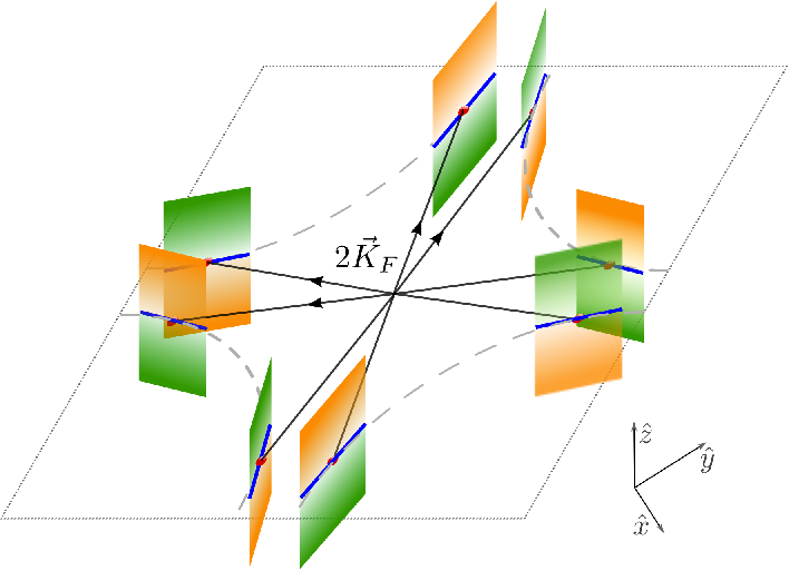
Figure 2: One-dimensional Fermi surfaces embedded in the three dimensional momentum space. The locally flat patches of two-dimensional Fermi surface near the hot spots are gapped out by the pzp_{z}-wave charge density wave carrying momentum 2​k→F2\vec{k}_{F} except for the line nodes at kzk_{z}=0.
Refer to caption
Figure 3: A patch of Fermi surface created by a pzp_{z}-wave CDW with momentum 2​k→F2\vec{k}_{F}. The center of the patch is pinched due to the CDW order that vanishes linearly in pzp_{z}. If the antiferromagnetic order parameter connects the pinched points, the low energy effective theory for the critical point becomes Eq. (2) in three dimensions.

The action supports one-dimensional Fermi surfaces embedded in dd-dimensional momentum space. The fermions have energy, En(k1,..,kd−2,k→)=±∑i=1d−2ki2+[εn​(k→)]2E_{n}(k_{1},..,k_{d-2},\vec{k})=\pm\sqrt{\sum_{i=1}^{d-2}k_{i}^{2}+[\varepsilon_{n}(\vec{k})]^{2}} which disperses linearly in the (d−1)(d-1)-dimensional space perpendicular to the line node defined by ki=0k_{i}=0 for 1≤i≤d−21\leq i\leq d-2 and εn​(k→)=0\varepsilon_{n}(\vec{k})=0. To understand the physical content of the dimensional regularization, it is useful to consider the theory at d=3d=3. With the choice of (γ0,γ1,γ2)=(σy,σz,σx)(\gamma_{0},\gamma_{1},\gamma_{2})=(\sigma_{y},\sigma_{z},\sigma_{x}) and identifying k1=kzk_{1}=k_{z}, the kinetic energy for Ψ1,σ\Psi_{1,\sigma} and Ψ3,σ\Psi_{3,\sigma} is written as H0=(vkx±ky)[ψ1,σ,j(±)∗ψ1,σ,j(±)−ψ3,σ,j(±)∗ψ3,σ,j(±)]∓kz[ψ1,σ,j(±)∗ψ3,σ,j(±)+h.c.]H_{0}=(vk_{x}\pm k_{y})\left[\psi^{(\pm)*}_{1,\sigma,j}\psi^{(\pm)}_{1,\sigma,j}-\psi^{(\pm)*}_{3,\sigma,j}\psi^{(\pm)}_{3,\sigma,j}\right]\mp k_{z}\left[\psi^{(\pm)*}_{1,\sigma,j}\psi^{(\pm)}_{3,\sigma,j}+h.c.\right]. The kinetic energy for Ψ2,σ\Psi_{2,\sigma} and Ψ4,σ\Psi_{4,\sigma} can be obtained by 90∘90^{\circ} rotation. The first term gives patches of locally flat two-dimensional Fermi surface. The second term describes a pzp_{z}-wave charge density wave (CDW) that gaps out the two-dimensional Fermi surface to leave line nodes at kz=0k_{z}=0, as is shown in Fig. 2. The full action in Eq. (2) describes the AF transition driven by electrons near the hot spots on the line nodes.

We emphasize that Eq. (2) is not just a mathematical construction. The theory in three space dimensions can arise at the AF quantum critical point in the presence of pzp_{z}-wave CDW of momentum 2​k→F2\vec{k}_{F}. If local curvature of the underlying Fermi surface is included, the dispersion near a pair of points on the Fermi surface connected by the momentum 2​k→F2\vec{k}_{F} can be written as ϵ±​(k→)=±kx+γ1​ky2+γ2​kz2\epsilon_{\pm}(\vec{k})=\pm k_{x}+\gamma_{1}k_{y}^{2}+\gamma_{2}k_{z}^{2}, where kxk_{x} is chosen to be perpendicular to the Fermi surface, and γi\gamma_{i} represent the local curvatures of the Fermi surface. The pzp_{z}-wave CDW leads to the spectrum, ℰ\mathcal{E} which is determined by |kx+γ1​ky2+γ2​kz2−ℰkzkz−kx+γ1​ky2+γ2​kz2−ℰ|=0.\begin{vmatrix}k_{x}+\gamma_{1}k_{y}^{2}+\gamma_{2}k_{z}^{2}-\mathcal{E}&k_{z}\\ k_{z}&-k_{x}+\gamma_{1}k_{y}^{2}+\gamma_{2}k_{z}^{2}-\mathcal{E}\end{vmatrix}=0. This results in a pinched Fermi surface located at γ1​ky2+γ2​kz2=kx2+kz2\gamma_{1}k_{y}^{2}+\gamma_{2}k_{z}^{2}=\sqrt{k_{x}^{2}+k_{z}^{2}} as is shown in Fig. 3. If the antiferromagnetic ordering wave vector connects the pinched points, the low energy effective theory for the phase transition is precisely described by Eq. (2) in three dimensions. Because the curvature is irrelevant at low energies, the pinched Fermi surfaces can be regarded as Fermi lines near the hot spots. Similar field theory can also arise at an orbital selective antiferromagnetic quantum critical point in three-dimensional semi-metal as is discussed in Appendix A.

The action in general dimensions respects the U⁡(1)U(1) charge conservation, the S​U​(Nc)SU(N_{c}) spin rotation, the S​U​(Nf)SU(N_{f}) flavor rotation, the 90∘90^{\circ} space rotation in (kx,ky)(k_{x},k_{y}), the reflections, and the time-reversal symmetries. For Nc=2N_{c}=2, the pseudospin symmetry, which rotates Ψn,σ,j​(k)\Psi_{n,\sigma,j}(k) into i​τσ,σ′(y)​γ0​Ψ¯n,σ′,jT​(−k)i\tau^{(y)}_{\sigma,\sigma^{\prime}}~\gamma_{0}\bar{\Psi}^{T}_{n,\sigma^{\prime},j}(-k), is present[22]. The action in Eq. (2) is also invariant under the S​O​(d−1)SO(d-1) rotation in 𝐊{\bf K}. In Appendix B we provide further details on symmetry.

The theory in 2≤d≤32\leq d\leq 3 continuously interpolates the physical theories which describe the AF critical points in d=2d=2 and 33. Because the couplings are marginal in three dimensions, we consider d=3−ϵd=3-\epsilon and expand around three space dimension using ϵ\epsilon as a small parameter. We use the field theoretic renormalization group scheme to compute the beta functions which govern the RG flow of the renormalized velocities and coupling constants.

By embedding the one-dimensional Fermi surface in higher dimensions, the density of state (DOS) is reduced to ρ⁡(E)∼Ed−2\rho(E)\sim E^{d-2}. As is the case for the usual dimensional regularization scheme for relativistic field theories, the reduced DOS tames quantum fluctuations at low energies and allows us to access low energy physics in a controlled way. Of course, there is no guarantee that the physics obtained near d=3d=3 is continuously extrapolated all the way to d=2d=2 because of the possibility that some operators that are irrelevant near d=3d=3 become relevant to drive instability near d=2d=2. However, it is our very goal to systematically examine the potential instability as dimension is lowered toward d=2d=2, for which we first need to establish the existence of stable fixed point at d=3d=3, which can be realized on its own.

Strange metal fixed point. We include one-loop quantum corrections to obtain the beta functions for the velocities and couplings (see Appendices C and D for computational details),

d​vd​l\displaystyle\frac{dv}{dl} =−(Nc2−1)2​Nc​Nf​π2​z​v​g2c​h2​(v,c),\displaystyle=-\frac{(N_{c}^{2}-1)}{2N_{c}N_{f}\pi^{2}}~\frac{z~v~g^{2}}{c}~h_{2}(v,c), (3)
d​cd​l\displaystyle\frac{dc}{dl} =−z​g28​π2​[π​cv−2​(Nc2−1)Nc​Nf​[h1​(v,c)−h2​(v,c)]],\displaystyle=-\frac{zg^{2}}{8\pi^{2}}~\left[\pi\frac{c}{v}-\frac{2(N_{c}^{2}-1)}{N_{c}N_{f}}[h_{1}(v,c)-h_{2}(v,c)]\right], (4)
d​gd​l\displaystyle\frac{dg}{dl} =z2​g​[ϵ−g24​π​v−g24​π3​Nc​Nf​c​{2​(Nc2−1)​π​h2​(v,c)−h3​(v,c)}],\displaystyle=\frac{z}{2}~g\left[\epsilon-\frac{g^{2}}{4\pi v}-\frac{g^{2}}{4\pi^{3}N_{c}N_{f}c}\left\{2(N_{c}^{2}-1)\pi~h_{2}(v,c)-h_{3}(v,c)\right\}\right], (5)
d​u1d​l\displaystyle\frac{du_{1}}{dl} =z​u12​c2​π2[c2π(2πϵ−g2v)+(Nc2−1)Nf​Nccg2{h1(v,c)−h2(v,c)}\displaystyle=\frac{zu_{1}}{2c^{2}\pi^{2}}\bigg[c^{2}\pi\left(2\pi\epsilon-\frac{g^{2}}{v}\right)+\frac{(N_{c}^{2}-1)}{N_{f}N_{c}}cg^{2}\{h_{1}(v,c)-h_{2}(v,c)\}
−(Nc2+7)u1−2​(2​Nc2−3)Ncu2−3(1+3Nc2)u22u1],\displaystyle-(N_{c}^{2}+7)u_{1}-\frac{2(2N_{c}^{2}-3)}{N_{c}}u_{2}-3\left(1+\frac{3}{N_{c}^{2}}\right)\frac{u_{2}^{2}}{u_{1}}\Bigg], (6)
d​u2d​l\displaystyle\frac{du_{2}}{dl} =z​u22​c2​π2​[c2​π​(2​π​ϵ−g2v)+(Nc2−1)Nf​Nc​c​g2​{h1​(v,c)−h2​(v,c)}−12​u1−2​(Nc2−9)Nc​u2].\displaystyle=\frac{zu_{2}}{2c^{2}\pi^{2}}\Bigg[c^{2}\pi\left(2\pi\epsilon-\frac{g^{2}}{v}\right)+\frac{(N_{c}^{2}-1)}{N_{f}N_{c}}cg^{2}\{h_{1}(v,c)-h_{2}(v,c)\}-12u_{1}-\frac{2(N_{c}^{2}-9)}{N_{c}}u_{2}\Bigg]. (7)

Here ll is the logarithmic length scale. z=[1−(Nc2−1)4​Nc​Nf​π2​g2c​{h1​(v,c)−h2​(v,c)}]−1z=\left[1-\frac{(N_{c}^{2}-1)}{4N_{c}N_{f}\pi^{2}}~\frac{g^{2}}{c}~\Bigl\{h_{1}(v,c)-h_{2}(v,c)\Bigr\}\right]^{-1} is the dynamical critical exponent that determines the scaling dimension of 𝐊{\bf K} relative to k→\vec{k}. hi​(v,c)h_{i}(v,c) are given by h1​(v,c)=∫01d​x​1−xc2+(1+v2−c2)​xh_{1}(v,c)=\int_{0}^{1}dx~\sqrt{\frac{1-x}{c^{2}+(1+v^{2}-c^{2})x}}, h2​(v,c)=c2​∫01d​x​1−x[c2+(1+v2−c2)​x]3h_{2}(v,c)=c^{2}\int_{0}^{1}dx~\sqrt{\frac{1-x}{\left[c^{2}+(1+v^{2}-c^{2})x\right]^{3}}} and h3​(v,c)=∫01d​x1​∫01−x1d​x2​∫02​πd​θ​[1ζ⁡(v,c,x1,x2,θ)−vc​sin⁡2​θζ2​(v,c,x1,x2,θ)]h_{3}(v,c)=\int_{0}^{1}dx_{1}\int_{0}^{1-x_{1}}dx_{2}\int_{0}^{2\pi}d\theta\left[\frac{1}{\zeta(v,c,x_{1},x_{2},\theta)}-\frac{v}{c}\frac{\sin{2\theta}}{\zeta^{2}(v,c,x_{1},x_{2},\theta)}\right] with

ζ⁡(v,c,x1,x2,θ)=2​vc​(x1​cos2⁡θ+x2​sin2⁡θ)+(1−x1−x2)​[v​c​cos2⁡(θ+π/4)+cv​sin2⁡(θ+π/4)].\zeta(v,c,x_{1},x_{2},\theta)=\frac{2v}{c}(x_{1}\cos^{2}{\theta}+x_{2}\sin^{2}{\theta})+(1-x_{1}-x_{2})\left[vc\cos^{2}(\theta+\pi/4)+\frac{c}{v}\sin^{2}(\theta+\pi/4)\right].
Refer to caption
(a)
Refer to caption
(b)
Figure 4: One-loop RG flow of the couplings and velocities for Nc=2N_{c}=2, Nf=1N_{f}=1 and ϵ=0.01\epsilon=0.01. We set u2=0u_{2}=0, which can be done without loss of generality for Nc<4N_{c}<4. The solid lines denote flows in the three-dimensional space of the parameters shown in the figure. The dashed lines represent flows within the subspace of g=0g=0. (a) The whole manifold of g=u1=0g=u_{1}=0 represents the non-interacting (Gaussian) fixed points parameterized by (v,c)(v,c). Once u1u_{1} is turned on at the Gaussian fixed points (denoted by circles), the theory flows to the Wilson-Fisher fixed points (squares). As the Yukawa coupling is introduced, couplings and velocities flow to the stable fixed point at g∗=ui∗=v∗=c∗=0g^{*}=u_{i}^{*}=v^{*}=c^{*}=0. (b) RG flow of the ratios of the parameters for the same values of NcN_{c}, NfN_{f} and ϵ\epsilon as in (a). The Yukawa coupling measured in the unit of v\sqrt{v} and the ratio of the two velocities remain non-zero at the stable fixed point.

The RG flow of the couplings and the velocities is shown in Fig. 4(a). We first examine the RG flow in the subspace of g=0g=0. At the Gaussian fixed points (ui=g=0u_{i}=g=0 with v,c≠0v,c\neq 0), the theory is free. With u1≠0u_{1}\neq 0 and u2=0u_{2}=0, the theory flows to the O⁡(Nc2−1)O(N_{c}^{2}-1) Wilson-Fisher (WF) fixed points at u1∗=2​π2​c2​ϵNc2+7u_{1}^{*}=\frac{2\pi^{2}c^{2}\epsilon}{N_{c}^{2}+7} with dynamical critical exponent z=1z=1. For Nc≥4N_{c}\geq 4, one also needs to consider u2u_{2}. As u2u_{2} is turned on, the O⁡(Nc2−1)O(N_{c}^{2}-1) WF fixed points become unstable and it shows a run-away flow[24] which suggests a first-order phase transition.

In the presence of Yukawa coupling, a stable low energy fixed point arises. If some components of the velocities were not allowed to flow, the theory could flow to a fixed point with finite couplings[25]. However, the full RG flow is more complicated because of running velocities. As gg is turned on, it initially grows as is expected from the fact that it is relevant below d=3d=3. As gg grows, the fermions at different hot spots are mixed with each other through quantum fluctuations. As a result, the hot spots become increasingly nested at low energies : vv flows to zero as 1/l1/l for ϵ>0\epsilon>0 and as 1/l​o​g​(l)1/log(l) for ϵ=0\epsilon=0 in the low energy limit. The dynamical nesting of the fermionic band, in turn, modifies the AF mode in two important ways. First, the boson becomes increasingly slow in the qx,qyq_{x},q_{y} directions because the collective mode can decay into dispersionless particle-hole pairs near the nested hot spots. As a result, cc decreases toward zero, leading to emergent locality in the (x,y)(x,y) space. Second, quantum fluctuations become more and more efficient in screening the interactions due to the abundant low energy density of states supported by the nested Fermi surface and the dispersionless boson. In summary of the RG flow, i) gg induces dynamical nesting, renormalizing v,cv,c to smaller values, ii) smaller v,cv,c make screening more efficient, making g,uig,u_{i} smaller. This cycle of negative feedback leaves no room for a coexistence of the kinetic terms (v,c)(v,c) and the interactions (g,ui)(g,u_{i}). It has only one fate down the road of RG flow : mutual destruction. To the one-loop order, all of v,c,g,uiv,c,g,u_{i} eventually flow to zero in the low energy limit at and below three dimensions if initial values of uiu_{i}’s are not too large in magnitude.

The new interactionless and quasi-dispersionless fixed point is distinct from the Gaussian fixed point which is dominated by the kinetic energy. Unlike at the Gaussian fixed point, the kinetic energy and the interactions maintain ‘a balance of power’ along the path to their demise. This can be seen from the fact that the ratios defined by

w≡vc,λ≡g2v,κi≡uic2\displaystyle w\equiv\frac{v}{c},~~\lambda\equiv\frac{g^{2}}{v},~~\kappa_{i}\equiv\frac{u_{i}}{c^{2}} (8)

flow to a stable fixed point,

w∗=Nc​NfNc2−1,λ∗=4​π​(Nc2+Nc​Nf−1)Nc2+Nc​Nf−3​ϵ,κi∗=0\displaystyle w^{*}=\frac{N_{c}N_{f}}{N_{c}^{2}-1},~~\lambda^{*}=\frac{4\pi(N_{c}^{2}+N_{c}N_{f}-1)}{N_{c}^{2}+N_{c}N_{f}-3}\epsilon,~~\kappa_{i}^{*}=0 (9)

in the c→0c\rightarrow 0 limit as is shown in Fig. 4(b). At the fixed point, the dynamical critical exponent is renormalized to z=1+λ∗8​πz=1+\frac{\lambda^{*}}{8\pi} to the leading order in λ\lambda. The non-trivial quantum correction to zz implies that the effect of interaction is not gone even though g,uig,u_{i} vanish in the low energy limit. This is due to the emergent locality associated with the dynamical nesting of the Fermi surface and the dispersionless bosonic spectrum. The IR singularity supported by the locality makes the system infinitely susceptible to interaction, leading to finite quantum corrections even with vanishing interactions. The fixed point is stable for general NcN_{c} and NfN_{f}, and small perturbations of ww, λ\lambda, κi\kappa_{i} away from Eq. (9) die out in the low energy limit. In particular, the ϕ4\phi^{4} vertices acquire an anomalous dimension and become irrelevant at the new fixed point. The one-loop fixed point is exact at d=3d=3 because higher order terms are systematically suppressed by λ\lambda and κi\kappa_{i} which flow to zero in the low energy limit. For d<3d<3, κi\kappa_{i}, cc, vv can receive higher-loop corrections to become nonzero at the fixed point. The details on higher-loop contributions can be found in Appendix E.

If the initial value of κ1\kappa_{1} is sufficiently large and negative, κ1\kappa_{1} runs away to −∞-\infty, potentially driving a first-order transition. The stable fixed point in Eq. (9) and the run-away flow is separated by an unstable fixed point at κ1∗=−4​π2​ϵ(Nc2+7)​(Nc2+Nc​Nf−3),κ2∗=0\kappa_{1}^{*}=-\frac{4\pi^{2}\epsilon}{(N_{c}^{2}+7)(N_{c}^{2}+N_{c}N_{f}-3)},\kappa_{2}^{*}=0 with the same values of w∗w^{*} and λ∗\lambda^{*} as in Eq. (9). The unstable fixed point, which can be realized at a multi-critical point, describes a state distinct from the state described by the stable fixed point in Eq. (9). The two fixed points are distinguished by the different ways the couplings and velocities approach the origin.

Physical properties. The existence of the stable low energy fixed point implies scale invariance of the Green’s function in the limit kx,ky,|𝐊|k_{x},k_{y},|{\bf K}| go to zero with kykx\frac{k_{y}}{k_{x}}, 𝐊|kx|z\frac{{\bf K}}{|k_{x}|^{z}} fixed at the second order phase transition. Here we focus on the Green’s function near the hot spot 1+1+ in Fig. 1. The Green’s function near other hot spots can be obtained by applying reflection or 90∘90^{\circ} rotation. In the scaling limit, the fermion Green’s function takes the form,

𝒢⁡(k)\displaystyle{\cal G}(k) =\displaystyle= 1|ky|1−2​η~ψ​G~​(𝐊|ky|z),\displaystyle\frac{1}{|k_{y}|^{1-2\tilde{\eta}_{\psi}}}\tilde{G}\left(\frac{{\bf K}}{|k_{y}|^{z}}\right), (10)

where η~ψ∼O⁡(ϵ2)\tilde{\eta}_{\psi}\sim O(\epsilon^{2}) is the net anomalous dimension which vanishes to the linear order in ϵ\epsilon and G~​(x)\tilde{G}(x) is a universal function. Because vv flows to zero logarithmically in the low energy limit, the dependence on kxk_{x} is suppressed as kxl​o​g​(1/kx)\frac{k_{x}}{log(1/k_{x})} for d<3d<3 and as kxl​o​g​(l​o​g​(1/kx))\frac{k_{x}}{log\left(log(1/k_{x})\right)} at d=3d=3 in the scaling limit. The dynamical critical exponent is non-trivial even to the linear order in ϵ\epsilon for d<3d<3. As a result, the spectral function shows a power-law distribution in energy instead of a delta function peak, exhibiting a non-Fermi liquid behavior. At d=3d=3, we have z=1z=1 as in Fermi liquid. However, the Green’s function is modified by logarithmic corrections compared to that of the Fermi liquid due to λ\lambda which flows to zero logarithmically. This is a marginal Fermi liquid[26]. Since the boson velocity also flows to zero in the same fashion vv flows to zero, the boson Green’s function becomes independent of kx,kyk_{x},k_{y} in the scaling limit upto corrections that are logarithmically suppressed,

𝒟⁡(k)\displaystyle{\cal D}(k) =\displaystyle= C|𝐊|2−2​η~ϕz,\displaystyle\frac{C}{|{\bf K}|^{\frac{2-2\tilde{\eta}_{\phi}}{z}}}, (11)

where CC is a constant and η~ϕ∼O⁡(ϵ2)\tilde{\eta}_{\phi}\sim O(\epsilon^{2}). This quasi-local strange metal supports non-quasiparticle excitations which are dispersionless along x,yx,y directions in the scaling limit. Here the effective space dimension becomes dynamically reduced as a result of quantum fluctuations. The quasi-local behaviors associated with extreme velocity anisotropies were reported in nodal semi-metals[27, 28]. Local critical behaviors with z=∞z=\infty also arise in the dynamical mean-field approximation for the Kondo lattice model[29] and from gravitational constructions[30, 31, 32]. The present quasi-local state is distinct from the earlier examples in that it is a stable zero temperature state which supports extended Fermi surface with a finite zz.

The quasi-local strange metal is stable at the one-loop order which becomes exact in the d→3d\rightarrow 3 limit. As one approaches d=2d=2, higher order corrections become important. The theory at d=2d=2 remains strongly coupled even in the large NcN_{c} and/or large NfN_{f} limit. One possibility is that the quasi-local strange metal becomes unstable towards an ordered state below a critical dimension. To identify the channels that may become unstable at d=2d=2, we examine charge density wave (CDW) and superconducting (SC) correlations that are enhanced by quantum fluctuations[22, 21]. In principle, particle-hole or particle-particle fluctuations between un-nested patches of Fermi surface may drive an instability if the coupling is strong at the lattice scale[34]. However, those operators that connect nested patches receive strongest quantum corrections.

In the spin-singlet CDW channel, the set of operators

OC​D​W±=∫d​k​[(Ψ¯1,σ,j​Ψ1,σ,j+Ψ¯3,σ,j​Ψ3,σ,j)±(Ψ¯2,σ,j​Ψ2,σ,j+Ψ¯4,σ,j​Ψ4,σ,j)]O_{CDW}^{\pm}=\int dk\left[\left(\bar{\Psi}_{1,\sigma,j}\Psi_{1,\sigma,j}+\bar{\Psi}_{3,\sigma,j}\Psi_{3,\sigma,j}\right)\pm\left(\bar{\Psi}_{2,\sigma,j}\Psi_{2,\sigma,j}+\bar{\Psi}_{4,\sigma,j}\Psi_{4,\sigma,j}\right)\right]

which describes a pyp_{y}-wave and a pxp_{x}-wave CDW, respectively, with momentum 2​k→F2\vec{k}_{F} is most strongly enhanced. These CDW operators, which are pseudospin singlets for Nc=2N_{c}=2, break the reflection symmetry and represent bond density waves without on-site modulation of charge. This is different from the bond density wave order which forms a pseudospin doublet with the d-wave pairing order [35]. In the SC channel, we focus on the representation that is symmetric in S​U​(Nf)SU(N_{f}) and anti-symmetric in S​U​(Nc)SU(N_{c}), which reduces to the spin-singlet SC order for Nc=2,Nf=1N_{c}=2,N_{f}=1. There are two sets of equally strong SC fluctuations. The first set of operators describes the dx2−y2d_{x^{2}-y^{2}}-wave and gg-wave pairings with zero momentum[36, 37], while the second set of operators describes ss-wave and dx​yd_{xy}-wave pairings with finite momentum, 2​k→F2\vec{k}_{F}[38, 39]. The attractive interaction for the pairing is mediated by the commensurate spin fluctuations that scatter a pair of electrons from one hot spot to another hot spot. Due to the nesting, the finite momentum pairing is as strong as the conventional zero momentum pairing to the one-loop order. The propensity for finite momentum pairing may lead to exotic superconducting states in two dimensions[40, 41]. If the quasi-local strange metal is unstable toward a competing order at low temperature in two dimensions, the strange metallic behaviors predicted in Eqs. (10) and (11) can show up within a finite temperature window whose range can be made parametrically large by tuning NcN_{c} and NfN_{f}[42]. For more details on the computation of the anomalous dimensions for the CDW and SC orders, please see Appendix F.

Within the perturbative regime that we explore in this paper, the anomalous dimensions for various susceptibilities associated with ‘hot’ electrons near the hot spots remain small. Because hot spots are only points in momentum space, thermodynamic and transport properties are dominated by cold electrons which exhibit Fermi liquid behaviors. For example, the specific heat will be proportional to T2−ϵT^{2-\epsilon} to the leading order of temperature TT, and the conductivity is expected to be dominated by cold electrons[33]. As one approaches d=2d=2, the contribution from hot electrons may, in principle, dominate over the contribution from the cold electrons as the anomalous dimensions become larger. Moreover, the behavior of cold electrons may also deviate from those of Fermi liquid far away from three dimensions, as the coupling between cold electrons and collective modes, which is irrelevant in the perturbative regime, becomes strong near d=2d=2[33]. In this case, non-Fermi liquid behavior may show up even for the thermodynamic and transport properties of cold electrons. However, we can not address this issue in a controlled manner because it requires strong coupling which lies outside the perturbative window.

Conclusion. We show that a novel strange metallic state emerges at the AF quantum critical point in a metal that supports one-dimensional Fermi surface based on a perturbative expansion which gives the exact low energy fixed point in three dimensions. Even though the interaction is screened to zero in the low energy limit, dynamical reduction of the effective dimensionality drives the system into a strange metallic state, which supports partially dispersionless incoherent single-particle excitations along with enhanced superconducting and charge density wave fluctuations. The present theory continuously interpolates between the three dimensional theory for one dimensional Fermi surfaces and two dimensional metals. The three-dimensional theory can arise at the AF quantum critical point in the presence of pzp_{z}-wave CDW, which is described by a stable quasi-local marginal Fermi liquid. Our formalism also provides a way to access potential instabilities of the non-Fermi liquids that arise at the AF quantum critical points below three dimensions as ϵ\epsilon increases.

Acknowledgements.
We thank Andrey Chubukov, Catherine Pepin, Patrick Lee, Max Metlitski, Subir Sachdev, T . Senthil and Yong Baek Kim for helpful discussions. The research was supported in part by the Natural Sciences and Engineering Research Council of Canada, the Early Research Award from the Ontario Ministry of Research and Innovation, and the Templeton Foundation. Research at the Perimeter Institute is supported in part by the Government of Canada through Industry Canada, and by the Province of Ontario through the Ministry of Research and Information.

Appendix A A three-dimensional lattice model for a related field theory

Refer to caption
(a)
Refer to caption
(b)
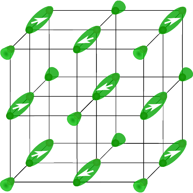
Figure 5: (a) Flux lattice in the X​YXY-plane. The green (dark) and the red (light) disks represent sites AA and BB, respectively. (b) Three dimensional arrangement of the AA and BB sites.

In this section we construct a three dimensional lattice model in which a field theory similar to the one considered in the main text can be realized. We consider a tetragonal lattice where staggered fluxes pierce through unit plaquettes. A gauge is chosen such that the hopping tzt_{z} along the zz direction is real. The nearest neighbor hoppings in the X​YXY-plane are written as {t1​ei​ϕ,t2​ei​ϕ}\{t_{1}e^{i\phi},t_{2}e^{i\phi}\} ({t1​e−i​ϕ,t2​e−i​ϕ})(\{t_{1}e^{-i\phi},t_{2}e^{-i\phi}\}) in the two orthogonal directions along (against) the arrows, as is shown in Figs. 5(a) and 5(b). Here the magnitudes of staggered flux per plaquette are (4​ϕ,2​ϕ,2​ϕ)(4\phi,2\phi,2\phi) in the three planes. In the coordinate system shown in Figs. 5(a) and 5(b), the lattice vectors become a→1=(1,0,0)\vec{a}_{1}=(1,0,0), a→2=(0,1,0)\vec{a}_{2}=(0,1,0), a→3=12​(1,1,1)\vec{a}_{3}=\frac{1}{2}(1,1,1), where the distance between nearest neighbor AA sites in the X​YXY-plane is chosen to be 11. The reciprocal vectors are given by b→1=2​π​(1,0,−1)\vec{b}_{1}=2\pi(1,0,-1), b→2=2​π​(0,1,−1)\vec{b}_{2}=2\pi(0,1,-1), b→3=4​π​(0,0,1)\vec{b}_{3}=4\pi(0,0,1).

Refer to caption
Figure 6: The (blue) curves represent the Fermi lines embedded in the three dimensional momentum space for Eq. (14) with t1=0.6​t2t_{1}=0.6~t_{2}. The (green) arrows represent the antiferromagnetic ordering vector with Q→=(π,π,0)\vec{Q}=(\pi,\pi,0). The shaded regions represent the kz=±πk_{z}=\pm\pi planes. There are four distinct hot spots connected by Q→\vec{Q} denoted by n=1,2,3,4n=1,2,3,4.

The tight binding Hamiltonian with the nearest neighbor hoppings becomes

H\displaystyle H =−∑k→[𝒟(k→)cA†(k→)cB(k→)+h.c.],\displaystyle=-\sum_{\vec{k}}\left[\mathcal{D}(\vec{k})~c^{{\dagger}}_{A}(\vec{k})~c_{B}(\vec{k})+h.c.\right], (12)

where cA⁡(B)c_{A(B)} is the destruction operator for electrons at AA (BB) sites, and

𝒟⁡(k→)\displaystyle\mathcal{D}(\vec{k}) =2​[cos⁡(ϕ)​{t+​cos⁡(kx2)​cos⁡(ky2)+t−​sin⁡(kx2)​sin⁡(ky2)}+tz​cos⁡(kz2)]\displaystyle=2\left[\cos(\phi)\left\{t_{+}\cos\left(\frac{k_{x}}{2}\right)\cos\left(\frac{k_{y}}{2}\right)+t_{-}\sin\left(\frac{k_{x}}{2}\right)\sin\left(\frac{k_{y}}{2}\right)\right\}+t_{z}\cos\left(\frac{k_{z}}{2}\right)\right]
+2​i​sin⁡(ϕ)​{t+​sin⁡(kx2)​sin⁡(ky2)+t−​cos⁡(kx2)​cos⁡(ky2)},\displaystyle\qquad+2i\sin(\phi)\left\{t_{+}\sin\left(\frac{k_{x}}{2}\right)\sin\left(\frac{k_{y}}{2}\right)+t_{-}\cos\left(\frac{k_{x}}{2}\right)\cos\left(\frac{k_{y}}{2}\right)\right\}, (13)

with t±=t1±t2t_{\pm}=t_{1}\pm t_{2}. The Hamiltonian is diagonal in spin indices, and we have suppressed the spin indices in the electron operators. The 2×22\times 2 Hamiltonian supports a particle-hole symmetric band with the dispersion E⁡(k→)=±|𝒟⁡(k→)|E(\vec{k})=\pm\left|{\mathcal{D}(\vec{k})}\right| at half filling. With the choice of 0<t1<t20<t_{1}<t_{2} and ϕ=π2\phi=\frac{\pi}{2}, one obtains one-dimensional Fermi surfaces (or Fermi lines) located at

kz=±π,\displaystyle k_{z}=\pm\pi,
sin⁡(kx2)​sin⁡(ky2)+t−t+​cos⁡(kx2)​cos⁡(ky2)=0.\displaystyle\sin\left(\frac{k_{x}}{2}\right)\sin\left(\frac{k_{y}}{2}\right)+\frac{t_{-}}{t_{+}}\cos\left(\frac{k_{x}}{2}\right)\cos\left(\frac{k_{y}}{2}\right)=0. (14)

The Fermi lines embedded in the three-dimensional momentum space are shown in Fig. 6.

Refer to caption
(a)
Refer to caption
(b)
Figure 7: A real space pattern for the orbital selective antiferromagnetic order (a) on the X​YXY plane and (b) in the full three dimensional lattice.

We assume that there exists an electron-electron interaction which drives the semi-metal into an antiferromagnetic state. In particular, we consider an orbital selective antiferromagnetic order, where electrons in the bonding and anti-bonding states within an unit cell have opposite spins, which then modulate with momentum (π,π,0)(\pi,\pi,0) in space. This is illustrated in Fig. 7. If the phase transition is continuous, the critical spin fluctuations associated with the order strongly interact with electrons on the Fermi lines connected by the ordering vector Q→=(π,π,0)\vec{Q}=(\pi,\pi,0) as is shown in Fig. 6. In this case, there exist four distinct hot spots connected by the ordering vector. As is considered in the main text, the minimal theory that describes the quantum critical point includes the electronic excitations near the hot spots and the critical antiferromagnetic mode that is coupled with electrons through the Yukawa coupling,

𝒮e​f​f\displaystyle\mathcal{S}_{eff} =∫d4​k(2​π)4​∑nΨ¯n​(k)​[i​k0​γ0+i​γ1​kz+i​γ2​εn​(k→)]​Ψn​(k→)\displaystyle=\int\frac{d^{4}k}{(2\pi)^{4}}\sum_{n}\bar{\Psi}_{n}(k)\left[ik_{0}\gamma_{0}+i\gamma_{1}k_{z}+i\gamma_{2}\varepsilon_{n}(\vec{k})\right]\Psi_{n}(\vec{k})
+ig0∫d4​k(2​π)4d4​q(2​π)4Φ→(q)⋅[Ψ¯1;s(k+q)γ2τ→s,s′Ψ4;s′(k)+Ψ¯2;s(k+q)γ2τ→s,s′Ψ3;s′(k)]+h.c.\displaystyle\quad+ig_{0}\int\frac{d^{4}k}{(2\pi)^{4}}\frac{d^{4}q}{(2\pi)^{4}}~\vec{\Phi}(q)\cdot\left[\bar{\Psi}_{1;s}(k+q)\gamma_{2}\vec{\tau}_{s,s^{\prime}}\Psi_{4;s^{\prime}}(k)+\bar{\Psi}_{2;s}(k+q)\gamma_{2}\vec{\tau}_{s,s^{\prime}}\Psi_{3;s^{\prime}}(k)\right]+h.c.
+12∫d4​q(2​π)4[q02+cz2qz2+cx2qx2+cy2qy2]Φ→(−q)⋅Φ→(q)\displaystyle\quad+\frac{1}{2}\int\frac{d^{4}q}{(2\pi)^{4}}\left[q_{0}^{2}+c_{z}^{2}q_{z}^{2}+c_{x}^{2}q_{x}^{2}+c_{y}^{2}q_{y}^{2}\right]\vec{\Phi}(-q)\cdot\vec{\Phi}(q)
+u04!∫d4​q1(2​π)4d4​q2(2​π)4d4​q3(2​π)4[Φ→(q1+q2)⋅Φ→(q2)][Φ→(q3−q2)⋅Φ→(q3)].\displaystyle\quad+\frac{u_{0}}{4!}\int\frac{d^{4}q_{1}}{(2\pi)^{4}}\frac{d^{4}q_{2}}{(2\pi)^{4}}\frac{d^{4}q_{3}}{(2\pi)^{4}}\left[\vec{\Phi}(q_{1}+q_{2})\cdot\vec{\Phi}(q_{2})\right]\left[\vec{\Phi}(q_{3}-q_{2})\cdot\vec{\Phi}(q_{3})\right]. (15)

Here Ψn​(k→)≡(cA​(K→n+k→)cB​(K→n+k→))\Psi_{n}(\vec{k})\equiv\left(\begin{array}[]{c}c_{A}(\vec{K}_{n}+\vec{k})\\ c_{B}(\vec{K}_{n}+\vec{k})\end{array}\right) with n=1,2,3,4n=1,2,3,4 denotes electrons near the nn-th hot spot with

K→1=(±π,0,±π),K→2=(0,±π,±π),K→3=(∓π,0,±π),K→4=(0,∓π,±π),\displaystyle\vec{K}_{1}=\left(\pm\pi,0,\pm\pi\right),\quad\vec{K}_{2}=\left(0,\pm\pi,\pm\pi\right),\quad\vec{K}_{3}=\left(\mp\pi,0,\pm\pi\right),\quad\vec{K}_{4}=\left(0,\mp\pi,\pm\pi\right), (16)

and Ψ¯n≡Ψn†​γ0\bar{\Psi}_{n}\equiv\Psi^{{\dagger}}_{n}\gamma_{0} with γ0=σz\gamma_{0}=\sigma_{z}, γ1=σy\gamma_{1}=\sigma_{y}, and γ2=σx\gamma_{2}=\sigma_{x}. εn​(k→)\varepsilon_{n}(\vec{k}) is the linearized dispersion around each hot spot,

ε1​(k→)=t−​kx−t+​ky,ε2​(k→)=−t+​kx+t−​ky,\displaystyle\varepsilon_{1}(\vec{k})=t_{-}k_{x}-t_{+}k_{y},\qquad\varepsilon_{2}(\vec{k})=-t_{+}k_{x}+t_{-}k_{y},
ε3​(k→)=−t−​kx+t+​ky,ε4​(k→)=t+​kx−t−​ky.\displaystyle\varepsilon_{3}(\vec{k})=-t_{-}k_{x}+t_{+}k_{y},\qquad\varepsilon_{4}(\vec{k})=t_{+}k_{x}-t_{-}k_{y}. (17)

We have scaled away tzt_{z} dependence by absorbing it in the z^\hat{z}-component of momentum. Φ→​(q)\vec{\Phi}(q) represents the critical fluctuations of the SDW order parameter.

Unlike the action in Eq. (2), Eq. (15) lacks the C4C_{4} symmetry in the X​YXY-plane and the S​O​(2)SO(2) rotation symmetry in the k0−kzk_{0}-k_{z} plane. This results in velocity anisotropy for the bosons. However, we expect that this theory also flows to a quasi-local fixed point similar to the one discussed in the main text[43].

Appendix B Symmetry

In this section, we elaborate on the symmetries of the action in Eq. (2). The internal symmetry is U​(1)2×S​U​(Nc)×S​U​(Nf)2U(1)^{2}\times SU(N_{c})\times SU(N_{f})^{2} associated with charge, spin and flavor conservations. There are two U⁡(1)U(1)’s and two S​U​(Nf)SU(N_{f})’s because the charge and flavor are conserved within the two sets of hot spots ({1,3}\{1,3\} and {2,4}\{2,4\}) separately. Besides the internal symmetry, the action has π/2\pi/2 rotation and reflection symmetries under which the spinors transform as is shown in the Table 1. In d>2d>2, the S​O​(d−1)SO(d-1) spacetime rotational symmetry is present. Under S​O​(d−1)SO(d-1) rotation, kμk_{\mu} and ψ¯n,σ,j​γμ​ψn,σ,j\bar{\psi}_{n,\sigma,j}\gamma_{\mu}\psi_{n,\sigma,j} form vectors for μ=0,1,…,d−2\mu=0,1,\ldots,d-2. For Nc=2N_{c}=2, there also exists a pseudo-spin symmetry under which the super-spinor, χn,σ,j​(k)=(Ψn,σ,j​(k),i​τσ,σ′(y)​γ0​Ψ¯n,σ′,jT​(−k))T\chi_{n,\sigma,j}(k)=\left(\Psi_{n,\sigma,j}(k),i\tau^{(y)}_{\sigma,\sigma^{\prime}}~\gamma_{0}~\bar{\Psi}^{T}_{n,\sigma^{\prime},j}(-k)\right)^{T} transforms as χn,σ,j↦U​χn,σ,j\chi_{n,\sigma,j}\mapsto U\chi_{n,\sigma,j}, where UU represents S​U​(2)SU(2) matrix that acts on the particle-hole space.

Rπ/2R_{\pi/2} RxR_{x} RyR_{y}
Ψ1​(k)\Psi_{1}(k) Ψ2​(kRπ/2)\Psi_{2}(k_{R_{\pi/2}}) −i​γ0​Ψ3​(kRx)-i\gamma_{0}\Psi_{3}(k_{R_{x}}) i​γ0​γd−1​Ψ3​(kRy)i\gamma_{0}\gamma_{d-1}\Psi_{3}(k_{R_{y}})
Ψ2​(k)\Psi_{2}(k) γd−1​Ψ1​(kRπ/2)\gamma_{d-1}\Psi_{1}(k_{R_{\pi/2}}) i​γ0​γd−1​Ψ4​(kRx)i\gamma_{0}\gamma_{d-1}\Psi_{4}(k_{R_{x}}) −i​γ0​Ψ4​(kRy)-i\gamma_{0}\Psi_{4}(k_{R_{y}})
Ψ3​(k)\Psi_{3}(k) Ψ4​(kRπ/2)\Psi_{4}(k_{R_{\pi/2}}) i​γ0​Ψ1​(kRx)i\gamma_{0}\Psi_{1}(k_{R_{x}}) i​γ0​γd−1​Ψ1​(kRy)i\gamma_{0}\gamma_{d-1}\Psi_{1}(k_{R_{y}})
Ψ4​(k)\Psi_{4}(k) −γd−1​Ψ3​(kRπ/2)-\gamma_{d-1}\Psi_{3}(k_{R_{\pi/2}}) i​γ0​γd−1​Ψ2​(kRx)i\gamma_{0}\gamma_{d-1}\Psi_{2}(k_{R_{x}}) i​γ0​Ψ2​(kRy)i\gamma_{0}\Psi_{2}(k_{R_{y}})
Table 1: Table of spinors obtained by applying the spatial π/2\pi/2 rotation and reflections in the xx and yy directions accompanied by reflections in k1,k2,…,kd−2k_{1},k_{2},\ldots,k_{d-2}. Under the three space symmetries, the energy-momentum vector k=(k0,k1,…,kd−2,kx,ky)k=(k_{0},k_{1},\ldots,k_{d-2},k_{x},k_{y}) is transformed to kRπ/2=(k0,k1,…,kd−2,−ky,kx)k_{R_{\pi/2}}=(k_{0},k_{1},\ldots,k_{d-2},-k_{y},k_{x}), kRx=(k0,−k1,…,−kd−2,−kx,ky)k_{R_{x}}=(k_{0},-k_{1},\ldots,-k_{d-2},-k_{x},k_{y}) and kRy=(k0,−k1,…,−kd−2,kx,−ky)k_{R_{y}}=(k_{0},-k_{1},\ldots,-k_{d-2},k_{x},-k_{y}), respectively. The spin and flavor indices are suppressed.

Appendix C Renormalization group analysis

In this section, we describe the method that is used to compute the beta functions for the velocities and couplings. In order to incorporate quantum corrections, we renormalize the theory by ‘tuning’ the parameters in the action in Eq. (2) such that the physical observables become insensitive to the UV cut-off scale. This amounts to adding counter terms that remove UV divergences in the quantum effective action order by order in the couplings. The internal and spacetime symmetries guarantee that the counter terms take the following form,

𝒮C​T\displaystyle\mathcal{S}_{CT} =∑n=14∑σ=1Nc∑j=1Nf∫dd+1​k(2​π)d+1​Ψ¯n,σ,j​(k)​[i​𝒜1​𝚪⋅𝐊+i​𝒜3​γd−1​εn​(k→,𝒜2𝒜3​v)]​Ψn,σ,j​(k)\displaystyle=\sum_{n=1}^{4}\sum_{\sigma=1}^{N_{c}}\sum_{j=1}^{N_{f}}\int\frac{d^{d+1}{k}}{(2\pi)^{d+1}}~\bar{\Psi}_{n,\sigma,j}(k)\left[i\mathcal{A}_{1}\mathbf{\Gamma}\cdot\mathbf{K}+i\mathcal{A}_{3}\gamma_{d-1}\varepsilon_{n}\left(\vec{k};\frac{\mathcal{A}_{2}}{\mathcal{A}_{3}}v\right)\right]\Psi_{n,\sigma,j}(k)
+14∫dd+1​q(2​π)d+1[𝒜4|𝐐|2+𝒜5c2|q→|2]Tr[Φ(−q)Φ(q)]\displaystyle+\frac{1}{4}\int\frac{d^{d+1}q}{(2\pi)^{d+1}}\Bigl[\mathcal{A}_{4}\left|{\mathbf{Q}}\right|^{2}+\mathcal{A}_{5}~c^{2}\left|{\vec{q}}\right|^{2}\Bigr]\mbox{Tr}\left[{\Phi(-q)~\Phi(q)}\right]
+i𝒜6g​μ(3−d)/2Nf∑n=14∑σ,σ′=1Nc∑j=1Nf∫dd+1​k(2​π)d+1dd+1​q(2​π)d+1[Ψ¯n¯,σ,j(k+q)Φσ,σ′(q)γd−1Ψn,σ′,j(k)]\displaystyle+i\mathcal{A}_{6}\frac{g\mu^{(3-d)/2}}{\sqrt{N_{f}}}\sum_{n=1}^{4}\sum_{\sigma,\sigma^{\prime}=1}^{N_{c}}\sum_{j=1}^{N_{f}}\int\frac{d^{d+1}{k}}{(2\pi)^{d+1}}\frac{d^{d+1}{q}}{(2\pi)^{d+1}}\Bigl[\bar{\Psi}_{\bar{n},\sigma,j}(k+q)\Phi_{\sigma,\sigma^{\prime}}(q)\gamma_{d-1}\Psi_{n,\sigma^{\prime},j}(k)\Bigr]
+μ3−d4∫dd+1​k1(2​π)d+1dd+1​k2(2​π)d+1dd+1​q(2​π)d+1[𝒜7u1Tr[Φ(k1+q)Φ(k2−q)]Tr[Φ(k1)Φ(k2)]\displaystyle+\frac{\mu^{3-d}}{4}\int\frac{d^{d+1}{k}_{1}}{(2\pi)^{d+1}}\frac{d^{d+1}{k}_{2}}{(2\pi)^{d+1}}\frac{d^{d+1}{q}}{(2\pi)^{d+1}}\Bigl[\mathcal{A}_{7}u_{1}\mbox{Tr}\left[{\Phi(k_{1}+q)\Phi(k_{2}-q)}\right]\mbox{Tr}\left[{\Phi(k_{1})\Phi(k_{2})}\right]
+𝒜8u2Tr[Φ(k1+q)Φ(k2−q)Φ(k1)Φ(k2)]],\displaystyle+\mathcal{A}_{8}u_{2}\mbox{Tr}\left[{\Phi(k_{1}+q)\Phi(k_{2}-q)\Phi(k_{1})\Phi(k_{2})}\right]\Bigl], (18)

where ε1​(k→,v)=v​kx+ky\varepsilon_{1}(\vec{k};v)=vk_{x}+k_{y}, ε2​(k→,v)=−kx+v​ky\varepsilon_{2}(\vec{k};v)=-k_{x}+vk_{y}, ε3​(k→,v)=v​kx−ky\varepsilon_{3}(\vec{k};v)=vk_{x}-k_{y}, and ε4​(k→,v)=kx+v​ky\varepsilon_{4}(\vec{k};v)=k_{x}+vk_{y}. In the minimal subtraction scheme, the counter terms only include contributions that are divergent in the ϵ→0\epsilon\rightarrow 0 limit,

𝒜n≡𝒜n​(v,c,g,u,ϵ)=∑m=1∞Zn,m​(v,c,g,u)ϵm,\displaystyle\mathcal{A}_{n}\equiv\mathcal{A}_{n}(v,c,g,u;\epsilon)=\sum_{m=1}^{\infty}\frac{Z_{n,m}(v,c,g,u)}{\epsilon^{m}}, (19)

where Zn,m​(v,c,g,u)Z_{n,m}(v,c,g,u) are finite functions of the couplings in the ϵ→0\epsilon\rightarrow 0 limit. The renormalized action is given by the sum of the original action and the counter terms, which can be expressed in terms of bare fields and bare couplings,

𝒮r​e​n\displaystyle\mathcal{S}_{ren} =∑n=14∑σ=1Nc∑j=1Nf∫dd+1​kB(2​π)d+1​Ψ¯B;n,σ,j​(kB)​[i​𝚪⋅𝐊B+i​γd−1​εn​(k→B,vB)]​ΨB;n,σ,j​(k)\displaystyle=\sum_{n=1}^{4}\sum_{\sigma=1}^{N_{c}}\sum_{j=1}^{N_{f}}\int\frac{d^{d+1}{k_{B}}}{(2\pi)^{d+1}}~\bar{\Psi}_{B;n,\sigma,j}(k_{B})\Bigl[i\mathbf{\Gamma}\cdot\mathbf{K}_{B}+i\gamma_{d-1}\varepsilon_{n}(\vec{k}_{B};v_{B})\Bigr]\Psi_{B;n,\sigma,j}(k)
+14∫dd+1​qB(2​π)d+1[|𝐐B|2+cB2|q→B|2]Tr[ΦB(−qB)ΦB(qB)]\displaystyle+\frac{1}{4}\int\frac{d^{d+1}q_{B}}{(2\pi)^{d+1}}\Bigl[\left|{\mathbf{Q}_{B}}\right|^{2}+~c_{B}^{2}\left|{\vec{q}_{B}}\right|^{2}\Bigr]\mbox{Tr}\left[{\Phi_{B}(-q_{B})~\Phi_{B}(q_{B})}\right]
+igBNf∑n=14∑σ,σ′=1Nc∑j=1Nf∫dd+1​kB(2​π)d+1dd+1​qB(2​π)d+1[Ψ¯B;n¯,σ,j(kB+qB)ΦB;σ,σ′(qB)γd−1ΨB;n,σ′,j(kB)]\displaystyle+i\frac{g_{B}}{\sqrt{N_{f}}}\sum_{n=1}^{4}\sum_{\sigma,\sigma^{\prime}=1}^{N_{c}}\sum_{j=1}^{N_{f}}\int\frac{d^{d+1}{k_{B}}}{(2\pi)^{d+1}}\frac{d^{d+1}{q_{B}}}{(2\pi)^{d+1}}\Bigl[\bar{\Psi}_{B;\bar{n},\sigma,j}(k_{B}+q_{B})\Phi_{B;\sigma,\sigma^{\prime}}(q_{B})\gamma_{d-1}\Psi_{B;n,\sigma^{\prime},j}(k_{B})\Bigr]
+14∫dd+1​k1​B(2​π)d+1dd+1​k2​B(2​π)d+1dd+1​qB(2​π)d+1[u1​BTr[ΦB(k1​B+qB)ΦB(k2​B−qB)]Tr[ΦB(k1​B)ΦB(k2​B)]\displaystyle+\frac{1}{4}\int\frac{d^{d+1}{k}_{1B}}{(2\pi)^{d+1}}\frac{d^{d+1}{k}_{2B}}{(2\pi)^{d+1}}\frac{d^{d+1}{q}_{B}}{(2\pi)^{d+1}}\Bigl[u_{1B}\mbox{Tr}\left[{\Phi_{B}(k_{1B}+q_{B})\Phi_{B}(k_{2B}-q_{B})}\right]\mbox{Tr}\left[{\Phi_{B}(k_{1B})\Phi_{B}(k_{2B})}\right]
+u2​BTr[ΦB(k1​B+qB)ΦB(k2​B−qB)ΦB(k1​B)ΦB(k2​B)]].\displaystyle+u_{2B}\mbox{Tr}\left[{\Phi_{B}(k_{1B}+q_{B})\Phi_{B}(k_{2B}-q_{B})\Phi_{B}(k_{1B})\Phi_{B}(k_{2B})}\right]\Bigr]. (20)

Here the renormalized quantities are related to the bare ones through

𝐊\displaystyle\mathbf{K} =𝒵τ−1​𝐊B,\displaystyle=\mathcal{Z}_{\tau}^{-1}~\mathbf{K}_{B}, k→\displaystyle\vec{k} =k→B,\displaystyle=\vec{k}_{B},
Ψn,σ,j​(k)\displaystyle\Psi_{n,\sigma,j}(k) =𝒵ψ−12​ΨB;n,σ,j​(kB),\displaystyle=\mathcal{Z}^{-\frac{1}{2}}_{\psi}~\Psi_{B;n,\sigma,j}(k_{B}), Φ⁡(q)\displaystyle\Phi(q) =𝒵ϕ−12​ΦB​(qB),\displaystyle=\mathcal{Z}^{-\frac{1}{2}}_{\phi}~\Phi_{B}(q_{B}),
v\displaystyle v =𝒵3𝒵2​vB,\displaystyle=\frac{\mathcal{Z}_{3}}{\mathcal{Z}_{2}}~v_{B}, c\displaystyle c =[𝒵ϕ​𝒵τd−1𝒵5]12​cB,\displaystyle=\left[\frac{\mathcal{Z}_{\phi}~\mathcal{Z}_{\tau}^{d-1}}{\mathcal{Z}_{5}}\right]^{\frac{1}{2}}~c_{B},
g\displaystyle g =𝒵ψ​𝒵ϕ12​𝒵τ2​(d−1)𝒵6​μ−3−d2​gB,\displaystyle=\frac{\mathcal{Z}_{\psi}~\mathcal{Z}_{\phi}^{\frac{1}{2}}~\mathcal{Z}_{\tau}^{2(d-1)}}{\mathcal{Z}_{6}}~\mu^{-\frac{3-d}{2}}~g_{B}, u1\displaystyle u_{1} =𝒵ϕ2​𝒵τ3​(d−1)𝒵7​μ−(3−d)​u1​B,\displaystyle=\frac{\mathcal{Z}_{\phi}^{2}\mathcal{Z}_{\tau}^{3(d-1)}}{\mathcal{Z}_{7}}~\mu^{-(3-d)}~u_{1B},
u2\displaystyle u_{2} =𝒵ϕ2​𝒵τ3​(d−1)𝒵8​μ−(3−d)​u2​B,\displaystyle=\frac{\mathcal{Z}_{\phi}^{2}\mathcal{Z}_{\tau}^{3(d-1)}}{\mathcal{Z}_{8}}~\mu^{-(3-d)}~u_{2B}, (21)

where 𝒵τ=𝒵1𝒵3\mathcal{Z}_{\tau}=\frac{\mathcal{Z}_{1}}{\mathcal{Z}_{3}}, 𝒵ψ=𝒵1​𝒵τ−d\mathcal{Z}_{\psi}=\mathcal{Z}_{1}~\mathcal{Z}_{\tau}^{-d}, and 𝒵ϕ=𝒵4​𝒵τ−(d+1)\mathcal{Z}_{\phi}=\mathcal{Z}_{4}~\mathcal{Z}_{\tau}^{-(d+1)} with 𝒵n=1+𝒜n\mathcal{Z}_{n}=1+\mathcal{A}_{n}. We use the freedom of choosing an overall scale to fix the scaling dimension of k→\vec{k} to be 11. The renormalized Green’s function defined through

⟨Ψ⁡(k1)​…​Ψ​(kf)​Ψ¯​(kf+1)​…​Ψ¯​(k2​f)​Φ​(q1)​…​Φ​(qb)⟩\displaystyle\langle\Psi(k_{1})\ldots\Psi(k_{f})\bar{\Psi}(k_{f+1})\ldots\bar{\Psi}(k_{2f})\Phi(q_{1})\ldots\Phi(q_{b})\rangle
=G(2​f,b)​(ki,qj,v,c,g,ui,μ)​δ(d+1)​(∑i=1f(ki−ki+f)+∑j=1bqj)\displaystyle\qquad=G^{(2f,b)}(k_{i},q_{j};v,c,g,u_{i},\mu)~\delta^{(d+1)}\left(\sum_{i=1}^{f}(k_{i}-k_{i+f})+\sum_{j=1}^{b}q_{j}\right) (22)

satisfies the renormalization group equation,

[z(𝐊i⋅∇𝐊i+𝐐j⋅∇𝐐j)+(k→i⋅∇→k→i+q→j⋅∇→q→j)−βv∂∂v−βc∂∂c−βg∂∂g−βui∂∂ui\displaystyle\left[z~\left(\mathbf{K}_{i}\cdot\mathbf{\nabla}_{\mathbf{K}_{i}}+\mathbf{Q}_{j}\cdot\mathbf{\nabla}_{\mathbf{Q}_{j}}\right)+\left(\vec{k}_{i}\cdot\vec{\nabla}_{\vec{k}_{i}}+\vec{q}_{j}\cdot\vec{\nabla}_{\vec{q}_{j}}\right)-\beta_{v}\frac{\partial}{\partial v}-\beta_{c}\frac{\partial}{\partial c}-\beta_{g}\frac{\partial}{\partial g}-\beta_{u_{i}}\frac{\partial}{\partial u_{i}}\right.
+2f(d+22−ηψ)+b(d+32−ηϕ)−(z(d−1)+2)]G(2​f,b)(ki,qi;v,c,g,ui,μ)=0.\displaystyle\quad\left.+2f\left(\frac{d+2}{2}-\eta_{\psi}\right)+b\left(\frac{d+3}{2}-\eta_{\phi}\right)-\left(z~(d-1)+2\right)\right]G^{(2f,b)}(k_{i},q_{i};v,c,g,u_{i},\mu)=0. (23)

Here the dynamical critical exponent and the anomalous dimensions of the fields are given by z=1+∂ln⁡𝒵τ∂ln⁡μz=1+\frac{\partial\ln{\mathcal{Z}_{\tau}}}{\partial\ln{\mu}}, ηψ=12​∂ln⁡𝒵ψ∂ln⁡μ\eta_{\psi}=\frac{1}{2}\frac{\partial\ln{\mathcal{Z}_{\psi}}}{\partial\ln{\mu}}, ηϕ=12​∂ln⁡𝒵ϕ∂ln⁡μ\eta_{\phi}=\frac{1}{2}\frac{\partial\ln{\mathcal{Z}_{\phi}}}{\partial\ln{\mu}}, and the beta functions that describe the flow of the parameters with increasing energy scale are given by βv=∂v∂ln⁡μ\beta_{v}=\frac{\partial v}{\partial\ln{\mu}}, βc=∂c∂ln⁡μ\beta_{c}=\frac{\partial c}{\partial\ln{\mu}}, βg=∂g∂ln⁡μ\beta_{g}=\frac{\partial g}{\partial\ln{\mu}}, βui=∂ui∂ln⁡μ\beta_{u_{i}}=\frac{\partial u_{i}}{\partial\ln{\mu}}. The set of coupled equations for the critical exponents and the beta functions can be rewritten as

𝒵3​[(d−1)​(z−1)+2​ηψ]−𝒵3′\displaystyle\mathcal{Z}_{3}\left[(d-1)(z-1)+2\eta_{\psi}\right]-\mathcal{Z}_{3}^{\prime} =0,\displaystyle=0,
𝒵1​[d⁡(z−1)+2​ηψ]−𝒵1′\displaystyle\mathcal{Z}_{1}\left[d(z-1)+2\eta_{\psi}\right]-\mathcal{Z}_{1}^{\prime} =0,\displaystyle=0,
𝒵4​[(d+1)​(z−1)+2​ηϕ]−𝒵4′\displaystyle\mathcal{Z}_{4}\left[(d+1)(z-1)+2\eta_{\phi}\right]-\mathcal{Z}_{4}^{\prime} =0,\displaystyle=0,
𝒵2​[βv−v⁡{(d−1)​(z−1)+2​ηψ}]+v​𝒵2′\displaystyle\mathcal{Z}_{2}\left[\beta_{v}-v\left\{(d-1)(z-1)+2\eta_{\psi}\right\}\right]+v\mathcal{Z}_{2}^{\prime} =0,\displaystyle=0,
𝒵5​[2​βc−c⁡{(d−1)​(z−1)+2​ηϕ}]+c​𝒵5′\displaystyle\mathcal{Z}_{5}\left[2\beta_{c}-c\left\{(d-1)(z-1)+2\eta_{\phi}\right\}\right]+c\mathcal{Z}_{5}^{\prime} =0,\displaystyle=0,
𝒵6​[βg−g⁡{−3−d2+2​(d−1)​(z−1)+2​ηψ+ηϕ}]+g​𝒵6′\displaystyle\mathcal{Z}_{6}\left[\beta_{g}-g\left\{-\frac{3-d}{2}+2(d-1)(z-1)+2\eta_{\psi}+\eta_{\phi}\right\}\right]+g\mathcal{Z}_{6}^{\prime} =0,\displaystyle=0,
𝒵7​[βu1−u1​{−(3−d)+3​(d−1)​(z−1)+4​ηϕ}]+u1​𝒵7′\displaystyle\mathcal{Z}_{7}\left[\beta_{u_{1}}-u_{1}\left\{-(3-d)+3(d-1)(z-1)+4\eta_{\phi}\right\}\right]+u_{1}\mathcal{Z}_{7}^{\prime} =0,\displaystyle=0,
𝒵8​[βu2−u2​{−(3−d)+3​(d−1)​(z−1)+4​ηϕ}]+u2​𝒵8′\displaystyle\mathcal{Z}_{8}\left[\beta_{u_{2}}-u_{2}\left\{-(3-d)+3(d-1)(z-1)+4\eta_{\phi}\right\}\right]+u_{2}\mathcal{Z}_{8}^{\prime} =0,\displaystyle=0,

which solve to give

z\displaystyle z =[1+(12g∂g+ui∂ui)(Z1,1−Z3,1)]−1,\displaystyle=\left[1+\left(\frac{1}{2}~g\partial_{g}+u_{i}\partial_{u_{i}}\right)(Z_{1,1}-Z_{3,1})\right]^{-1}, (25)
ηψ\displaystyle\eta_{\psi} =−ϵ2z(12g∂g+ui∂ui)(Z1,1−Z3,1)+12z(12g∂g+ui∂ui)(2Z1,1−3Z3,1),\displaystyle=-\frac{\epsilon}{2}~z\left(\frac{1}{2}~g\partial_{g}+u_{i}\partial_{u_{i}}\right)\left(Z_{1,1}-Z_{3,1}\right)+\frac{1}{2}~z\left(\frac{1}{2}~g\partial_{g}+u_{i}\partial_{u_{i}}\right)\left(2Z_{1,1}-3Z_{3,1}\right), (26)
ηϕ\displaystyle\eta_{\phi} =−ϵ2z(12g∂g+ui∂ui)(Z1,1−Z3,1)+12z(12g∂g+ui∂ui)(4Z1,1−4Z3,1−Z4,1),\displaystyle=-\frac{\epsilon}{2}~z\left(\frac{1}{2}~g\partial_{g}+u_{i}\partial_{u_{i}}\right)\left(Z_{1,1}-Z_{3,1}\right)+\frac{1}{2}~z\left(\frac{1}{2}~g\partial_{g}+u_{i}\partial_{u_{i}}\right)\left(4Z_{1,1}-4Z_{3,1}-Z_{4,1}\right), (27)
βv\displaystyle\beta_{v} =zv(12g∂g+ui∂ui)(Z2,1−Z3,1),\displaystyle=z~v\left(\frac{1}{2}~g\partial_{g}+u_{i}\partial_{u_{i}}\right)\left(Z_{2,1}-Z_{3,1}\right), (28)
βc\displaystyle\beta_{c} =12zc(12g∂g+ui∂ui)(2Z1,1−2Z3,1−Z4,1+Z5,1),\displaystyle=\frac{1}{2}~z~c\left(\frac{1}{2}~g\partial_{g}+u_{i}\partial_{u_{i}}\right)\left(2Z_{1,1}-2Z_{3,1}-Z_{4,1}+Z_{5,1}\right), (29)
βg\displaystyle\beta_{g} =−zg[ϵ2+12(12g∂g+ui∂ui)(2Z3,1+Z4,1−2Z6,1)],\displaystyle=-z~g\left[\frac{\epsilon}{2}+\frac{1}{2}\left(\frac{1}{2}~g\partial_{g}+u_{i}\partial_{u_{i}}\right)\left(2Z_{3,1}+Z_{4,1}-2Z_{6,1}\right)\right], (30)
βu1\displaystyle\beta_{u_{1}} =−zu1[ϵ−(12g∂g+ui∂ui)(2Z1,1−2Z3,1−2Z4,1+Z7,1)],\displaystyle=-z~u_{1}\left[\epsilon-\left(\frac{1}{2}~g\partial_{g}+u_{i}\partial_{u_{i}}\right)\left(2Z_{1,1}-2Z_{3,1}-2Z_{4,1}+Z_{7,1}\right)\right], (31)
βu2\displaystyle\beta_{u_{2}} =−zu2[ϵ−(12g∂g+ui∂ui)(2Z1,1−2Z3,1−2Z4,1+Z8,1)].\displaystyle=-z~u_{2}\left[\epsilon-\left(\frac{1}{2}~g\partial_{g}+u_{i}\partial_{u_{i}}\right)\left(2Z_{1,1}-2Z_{3,1}-2Z_{4,1}+Z_{8,1}\right)\right]. (32)
Refer to caption
(a)
Refer to caption
(b)
Refer to caption
(c)
Refer to caption
(d)
Refer to caption
(e)
Figure 8: One-loop Feynman diagrams that contribute to the quantum effective action. Solid (wiggly) lines represent the fermion (boson) propagator. Cubic vertices represent the Yukawa coupling, gg. In (e), each quartic vertex can be either u1u_{1} and u2u_{2}.

The counter terms can be computed order by order in the loop expansion. We include the contributions from the one-loop diagrams shown in Fig. 8. The computations of the diagrams are discussed in the next section of this supplementary material. Here we summarize the final results,

Z1,1\displaystyle Z_{1,1} =−(Nc2−1)4​π2​Nc​Nf​g2c​h1​(v,c),\displaystyle=-\frac{(N_{c}^{2}-1)}{4\pi^{2}N_{c}N_{f}}~\frac{g^{2}}{c}~h_{1}(v,c),
Z2,1\displaystyle Z_{2,1} =(Nc2−1)4​π2​Nc​Nf​g2c​h2​(v,c),\displaystyle=\frac{(N_{c}^{2}-1)}{4\pi^{2}N_{c}N_{f}}~\frac{g^{2}}{c}~h_{2}(v,c),
Z3,1\displaystyle Z_{3,1} =−Z2,1,\displaystyle=-Z_{2,1},
Z4,1\displaystyle Z_{4,1} =−14​π​g2v,\displaystyle=-\frac{1}{4\pi}~\frac{g^{2}}{v},
Z5,1\displaystyle Z_{5,1} =0,\displaystyle=0,
Z6,1\displaystyle Z_{6,1} =−18​π3​Nc​Nf​g2c​h3​(v,c),\displaystyle=-\frac{1}{8\pi^{3}N_{c}N_{f}}~\frac{g^{2}}{c}~h_{3}(v,c),
Z7,1\displaystyle Z_{7,1} =12​π2​c2​[(Nc2+7)​u1+2​(2​Nc−3Nc)​u2+3​(1+3Nc2)​u22u1],\displaystyle=\frac{1}{2\pi^{2}c^{2}}\left[(N_{c}^{2}+7)u_{1}+2\left(2N_{c}-\frac{3}{N_{c}}\right)u_{2}+3\left(1+\frac{3}{N_{c}^{2}}\right)\frac{u_{2}^{2}}{u_{1}}\right],
Z8,1\displaystyle Z_{8,1} =12​π2​c2​[12​u1+2​(Nc−9Nc)​u2],\displaystyle=\frac{1}{2\pi^{2}c^{2}}\left[12u_{1}+2\left(N_{c}-\frac{9}{N_{c}}\right)u_{2}\right], (33)

where hi​(v,c)h_{i}(v,c) are defined in the main text. This gives the beta functions and the dynamical critical exponent shown in Eqs. (3)-(7) and below. The anomalous dimensions of the fields are given by

ηψ\displaystyle\eta_{\psi} =z​(Nc2−1)8​π2​Nc​Nf​g2c​[ϵ⁡{h1​(v,c)−h2​(v,c)}−{2​h1​(v,c)−3​h2​(v,c)}],\displaystyle=z~\frac{(N_{c}^{2}-1)}{8\pi^{2}N_{c}N_{f}}~\frac{g^{2}}{c}~\left[\epsilon~\Bigl\{h_{1}(v,c)-h_{2}(v,c)\Bigr\}-\Bigl\{2h_{1}(v,c)-3h_{2}(v,c)\Bigr\}\right], (34)
ηϕ\displaystyle\eta_{\phi} =z8​π​g2c​[cv−(4−ϵ)​(Nc2−1)π​Nc​Nf​{h1​(v,c)−h2​(v,c)}].\displaystyle=\frac{z}{8\pi}\frac{g^{2}}{c}\left[\frac{c}{v}-(4-\epsilon)\frac{(N_{c}^{2}-1)}{\pi N_{c}N_{f}}~\Bigl\{h_{1}(v,c)-h_{2}(v,c)\Bigr\}\right]. (35)

It is noted that the beta functions used in the main text describe the flow of the couplings with increasing length scale, which is defined to be ∂g∂l≡−βg\frac{\partial g}{\partial l}\equiv-\beta_{g}.

Because all v,c,g,uiv,c,g,u_{i} flow to zero in the low energy limit as discussed in the main text, it is more convenient to consider the ratios of the couplings, w=vcw=\frac{v}{c}, λ=g2v\lambda=\frac{g^{2}}{v} and κi=uic2\kappa_{i}=\frac{u_{i}}{c^{2}}. The beta functions for the ratios are given by

∂w∂l\displaystyle\frac{\partial{w}}{\partial{l}} =z​w​λ8​π​[1−2​w​(Nc2−1)π​Nc​Nf​{h1​(w​c,c)+h2​(w​c,c)}],\displaystyle=\frac{zw\lambda}{8\pi}\left[1-\frac{2w(N_{c}^{2}-1)}{\pi N_{c}N_{f}}\Bigl\{h_{1}(wc,c)+h_{2}(wc,c)\Bigr\}\right], (36)
∂λ∂l\displaystyle\frac{\partial{\lambda}}{\partial{l}} =z​λ​[ϵ−λ4​π​{1−wπ2​Nc​Nf​h3​(w​c,w)}],\displaystyle=z~\lambda\left[\epsilon-\frac{\lambda}{4\pi}\left\{1-\frac{w}{\pi^{2}N_{c}N_{f}}~h_{3}(wc,w)\right\}\right], (37)
∂κ1∂l\displaystyle\frac{\partial{\kappa_{1}}}{\partial{l}} =z​κ1​[{ϵ−λ4​π}−(Nc2+7)2​π2​κ1−(2​Nc2−3)π2​Nc​κ2−3​(Nc2+3)2​π2​Nc2​κ22κ1],\displaystyle=z~\kappa_{1}\left[\left\{\epsilon-\frac{\lambda}{4\pi}\right\}-\frac{(N_{c}^{2}+7)}{2\pi^{2}}~\kappa_{1}-\frac{(2N_{c}^{2}-3)}{\pi^{2}N_{c}}~\kappa_{2}-\frac{3(N_{c}^{2}+3)}{2\pi^{2}N_{c}^{2}}\frac{\kappa_{2}^{2}}{\kappa_{1}}\right], (38)
∂κ2∂l\displaystyle\frac{\partial{\kappa_{2}}}{\partial{l}} =z​κ2​[{ϵ−λ4​π}−6π2​κ1−Nc2−9π2​Nc​κ2].\displaystyle=z~\kappa_{2}\left[\left\{\epsilon-\frac{\lambda}{4\pi}\right\}-\frac{6}{\pi^{2}}~\kappa_{1}-\frac{N_{c}^{2}-9}{\pi^{2}N_{c}}~\kappa_{2}\right]. (39)

By using limc→0h1​(w​c,c)=π2\lim_{c\rightarrow 0}h_{1}(wc,c)=\frac{\pi}{2}, limc→0h2​(w​c,c)=0\lim_{c\rightarrow 0}h_{2}(wc,c)=0 and limc→0h3​(w​c,c)=2​π21+w\lim_{c\rightarrow 0}h_{3}(wc,c)=\frac{2\pi^{2}}{1+w}, it can be shown that the beta functions for cc, ww, λ\lambda and κi\kappa_{i} simultaneously vanish at the attractive fixed point given in Eq. (9). At the fixed point, the dynamical critical exponent and the anomalous dimensions are given by

z\displaystyle z =\displaystyle= 1+Nc2+Nc​Nf−12​(Nc2+Nc​Nf−3)​ϵ,\displaystyle 1+\frac{N_{c}^{2}+N_{c}N_{f}-1}{2(N_{c}^{2}+N_{c}N_{f}-3)}\epsilon,
ηψ=ηϕ\displaystyle\eta_{\psi}=\eta_{\phi} =\displaystyle= −Nc2+Nc​Nf−12​(Nc2+Nc​Nf−3)​ϵ\displaystyle-\frac{N_{c}^{2}+N_{c}N_{f}-1}{2(N_{c}^{2}+N_{c}N_{f}-3)}\epsilon (40)

to the leading order in ϵ\epsilon. Both the dynamical critical exponent and the anomalous dimensions modify the scaling of the renormalized Green’s function as can be checked from Eq. (23). As a result, the two-point functions in Eqs. (10) and (11) are controlled by the net anomalous dimensions defined by η~ψ=ηψ+(z−1)​(2−ϵ)2\tilde{\eta}_{\psi}=\eta_{\psi}+\frac{(z-1)(2-\epsilon)}{2}, η~ϕ=ηϕ+(z−1)​(2−ϵ)2\tilde{\eta}_{\phi}=\eta_{\phi}+\frac{(z-1)(2-\epsilon)}{2}, which vanish to the linear order in ϵ\epsilon. It is expected that there will be non-trivial anomalous dimensions for the two-point functions beyond the one-loop level[14]. Higher-point correlation functions exhibit non-trivial anomalous dimensions even to the linear order in ϵ\epsilon because the quantum corrections are not canceled in Eq. (23) for 2​f+b>22f+b>2.

Appendix D Computation of one-loop diagrams

In this section, we outline the computations of the one-loop Feynman diagrams that result in Eq. (33). We will use δ​S\delta S to denote the contributions to the quantum effective action, and SC​TS_{CT} to denote the counter terms that are needed to cancel the UV divergent pieces in δ​S\delta S in the ϵ→0\epsilon\rightarrow 0 limit.

D.1 Fermion self energy

The quantum correction to the fermion self-energy from the diagram in Fig. 8(a) is

δ​𝒮(2,0)\displaystyle\delta\mathcal{S}^{(2,0)} =2​g2​μ3−dNf​(Nc−1Nc)​∑n=14∑σ=1Nc∑j=1Nf∫dd+1​k(2​π)d+1​Ψ¯n,σ,j​(k)​Υ(2,0)(n)​(k)​Ψn,σ,j​(k),\displaystyle=\frac{2g^{2}\mu^{3-d}}{N_{f}}\left(N_{c}-\frac{1}{N_{c}}\right)\sum_{n=1}^{4}\sum_{\sigma=1}^{N_{c}}\sum_{j=1}^{N_{f}}\int\frac{d^{d+1}k}{(2\pi)^{d+1}}~\bar{\Psi}_{n,\sigma,j}(k)~\Upsilon_{(2,0)}^{(n)}(k)~\Psi_{n,\sigma,j}(k), (41)

where

Υ(2,0)(n)​(k)\displaystyle\Upsilon_{(2,0)}^{(n)}(k) =∫dd−1​𝐐(2​π)d−1​d2​q→(2​π)2​γd−1​Gn¯​(k+q)​γd−1​D​(q),\displaystyle=\int\frac{d^{d-1}\mathbf{Q}}{(2\pi)^{d-1}}\frac{d^{2}\vec{q}}{(2\pi)^{2}}~\gamma_{d-1}G_{\bar{n}}(k+q)\gamma_{d-1}~D(q), (42)

and the bare Green’s functions are given by

Gn​(k)=−i​𝚪⋅𝐊+γd−1​εn​(k→)|𝐊|2+εn2​(k→),\displaystyle G_{n}(k)=-i~\frac{\mathbf{\Gamma}\cdot\mathbf{K}+\gamma_{d-1}\varepsilon_{n}(\vec{k})}{\left|{\mathbf{K}}\right|^{2}+\varepsilon_{n}^{2}(\vec{k})}, (43)
D⁡(q)=1|𝐐|2+c2​|q→|2.\displaystyle D(q)=\frac{1}{\left|{\mathbf{Q}}\right|^{2}+c^{2}\left|{\vec{q}}\right|^{2}}. (44)

After the integrations over q→\vec{q} and 𝐐{\bf Q}, Eq. (42) can be expressed in terms of a Feynman parameter,

Υ(2,0)(n)​(k)\displaystyle\Upsilon_{(2,0)}^{(n)}(k) =i(4​π)(d+1)/2​c​Γ​(3−d2)​∫01d​x​1−xc2+x⁡(1+v2−c2)\displaystyle=\frac{i}{(4\pi)^{(d+1)/2}c}\Gamma\left(\frac{3-d}{2}\right)\int_{0}^{1}dx~\sqrt{\frac{1-x}{c^{2}+x(1+v^{2}-c^{2})}}
×[x⁡(1−x)​{|𝐊|2+c2​εn¯2​(k→)c2+x⁡(1+v2−c2)}]−3−d2​[𝐊⋅𝚪−c2​εn¯​(k→)​γd−1c2+x⁡(1+v2−c2)].\displaystyle\times\left[x(1-x)\left\{|\mathbf{K}|^{2}+\frac{c^{2}\varepsilon_{\bar{n}}^{2}(\vec{k})}{c^{2}+x(1+v^{2}-c^{2})}\right\}\right]^{-\frac{3-d}{2}}\left[\mathbf{K}\cdot\mathbf{\Gamma}-\frac{c^{2}~\varepsilon_{\bar{n}}(\vec{k})~\gamma_{d-1}}{c^{2}+x(1+v^{2}-c^{2})}\right]. (45)

The UV divergent part in the ϵ→0\epsilon\rightarrow 0 limit is given by

Υ(2,0)(n)​(k)=i8​π2​c​ϵ​[h1​(v,c)​𝐊⋅𝚪−h2​(v,c)​εn¯​(k→)​γd−1],\Upsilon_{(2,0)}^{(n)}(k)=\frac{i}{8\pi^{2}~c~\epsilon}\left[h_{1}(v,c)~\mathbf{K}\cdot\mathbf{\Gamma}-h_{2}(v,c)~\varepsilon_{\bar{n}}(\vec{k})\gamma_{d-1}\right],

where h1​(v,c)=∫01d​x​1−xc2+(1+v2−c2)​xh_{1}(v,c)=\int_{0}^{1}dx~\sqrt{\frac{1-x}{c^{2}+(1+v^{2}-c^{2})x}}, h2​(v,c)=c2​∫01d​x​1−x(c2+(1+v2−c2)​x)3h_{2}(v,c)=c^{2}\int_{0}^{1}dx~\sqrt{\frac{1-x}{(c^{2}+(1+v^{2}-c^{2})x)^{3}}}. This leads to the one-loop counter term for the fermion self-energy,

𝒮C​T(2,0)\displaystyle\mathcal{S}^{(2,0)}_{CT} =−ig24​π2​c​ϵNc2−1Nf​Nc∑n=14∑σ=1Nc∑j=1Nf∫dd+1​k(2​π)d+1\displaystyle=-i\frac{g^{2}}{4\pi^{2}c\epsilon}\frac{N_{c}^{2}-1}{N_{f}N_{c}}\sum_{n=1}^{4}\sum_{\sigma=1}^{N_{c}}\sum_{j=1}^{N_{f}}\int\frac{d^{d+1}k}{(2\pi)^{d+1}}~
×Ψ¯n,σ,j​(k)​[h1​(v,c)​𝐊⋅𝚪−h2​(v,c)​εn¯​(k→)​γd−1]​Ψn,σ,j​(k).\displaystyle\qquad\qquad\times\bar{\Psi}_{n,\sigma,j}(k)\left[h_{1}(v,c)~\mathbf{K}\cdot\mathbf{\Gamma}-h_{2}(v,c)~\varepsilon_{\bar{n}}(\vec{k})\gamma_{d-1}\right]\Psi_{n,\sigma,j}(k). (46)

D.2 Boson self energy

The boson self energy in Fig. 8(b) is given by

δ​𝒮(0,2)\displaystyle\delta\mathcal{S}^{(0,2)} =−2g2μ3−d∑a∫dd+1​q(2​π)d+1Υ(0,2)(q)ϕa(−q)ϕa(q),\displaystyle=-2g^{2}\mu^{3-d}\sum_{a}\int\frac{d^{d+1}q}{(2\pi)^{d+1}}~\Upsilon_{(0,2)}(q)~{\phi}^{a}(-q){\phi}^{a}(q), (47)

where

Υ(0,2)​(q)\displaystyle\Upsilon_{(0,2)}(q) =12​∑n∫dd−1​𝐊(2​π)d−1​d2​k→(2​π)2​Tr​[γd−1​Gn¯​(k+q)​γd−1​Gn​(k)].\displaystyle=\frac{1}{2}\sum_{n}\int\frac{d^{d-1}\mathbf{K}}{(2\pi)^{d-1}}\frac{d^{2}\vec{k}}{(2\pi)^{2}}~\mbox{Tr}\left[\gamma_{d-1}G_{\bar{n}}(k+q)\gamma_{d-1}G_{n}(k)\right]. (48)

We first integrate over k→\vec{k}. Using the Feynman parameterization, we write the resulting expression as

Υ(0,2)​(q)\displaystyle\Upsilon_{(0,2)}(q) =12​π​v​∫01d​x​∫dd−1​𝐊(2​π)d−1​[x⁡(1−x)]−12​𝐊⋅(𝐊+𝐐)x​|𝐊+𝐐|2+(1−x)​|𝐊|2.\displaystyle=\frac{1}{2\pi v}\int_{0}^{1}dx\int\frac{d^{d-1}\mathbf{K}}{(2\pi)^{d-1}}~\frac{[x(1-x)]^{-\frac{1}{2}}~~\mathbf{K}\cdot(\mathbf{K}+\mathbf{Q})}{x\left|{\mathbf{K}+\mathbf{Q}}\right|^{2}+(1-x)\left|{\mathbf{K}}\right|^{2}}. (49)

The quadratically divergent term is the mass renormalization, which is automatically tuned away at the critical point in the present scheme. The remaining correction to the kinetic energy of the boson becomes Υ(0,2)​(q)=−|𝐐|216​π​v​ϵ\Upsilon_{(0,2)}(q)=-\frac{\left|{\mathbf{Q}}\right|^{2}}{16\pi v\epsilon} up to finite terms. Accordingly we add the following counter term,

𝒮C​T(0,2)\displaystyle\mathcal{S}^{(0,2)}_{CT} =−∑ag28​π​v​ϵ∫dd+1​q(2​π)d+1|𝐐|2ϕa(−q)ϕa(q).\displaystyle=-\sum_{a}\frac{g^{2}}{8\pi v\epsilon}\int\frac{d^{d+1}q}{(2\pi)^{d+1}}~\left|{\mathbf{Q}}\right|^{2}~{\phi}^{a}(-q){\phi}^{a}(q). (50)

D.3 Yukawa vertex correction

The diagram in Fig. 8(c) gives rise to the vertex correction in the quantum effective action,

δ​𝒮(2,1)\displaystyle\delta\mathcal{S}^{(2,1)} =i​2​g3​μ32​(3−d)Nc​Nf3/2​∑a,n∑j,σ,σ′∫dd+1​k(2​π)d+1​dd+1​q(2​π)d+1​ϕa​(q)​Ψ¯n,σ,j​(k+q)​τσ,σ′a​Υ(2,1)(n)​(k,q)​Ψn¯,σ′,j​(k),\displaystyle=i\frac{2g^{3}\mu^{\frac{3}{2}(3-d)}}{N_{c}N_{f}^{3/2}}\sum_{a,n}\sum_{j,\sigma,\sigma^{\prime}}\int\frac{d^{d+1}{k}}{(2\pi)^{d+1}}\frac{d^{d+1}{q}}{(2\pi)^{d+1}}~{\phi}^{a}(q)\bar{\Psi}_{n,\sigma,j}(k+q){\tau}^{a}_{\sigma,\sigma^{\prime}}\Upsilon^{(n)}_{(2,1)}(k,q)~\Psi_{\bar{n},\sigma^{\prime},j}(k), (51)

where

Υ(2,1)(n)​(k,q)\displaystyle\Upsilon^{(n)}_{(2,1)}(k,q) =∫dd−1​𝐏(2​π)d−1​d2​p→(2​π)2​γd−1​Gn¯​(p+q+k)​γd−1​Gn​(p+k)​γd−1​D​(p).\displaystyle=\int\frac{d^{d-1}\mathbf{P}}{(2\pi)^{d-1}}\frac{d^{2}\vec{p}}{(2\pi)^{2}}~\gamma_{d-1}G_{\bar{n}}(p+q+k)\gamma_{d-1}G_{n}(p+k)\gamma_{d-1}~D(p). (52)

Here we use the identity for the S​U​(Nc)SU(N_{c}) generators, ∑a=1Nc2−1τa​τb​τa=−2Nc​τb\sum_{a=1}^{N_{c}^{2}-1}\tau^{a}\tau^{b}\tau^{a}=-\frac{2}{N_{c}}~\tau^{b}. The UV divergent part in the ϵ→0\epsilon\rightarrow 0 limit, which can be extracted by setting all external frequency and momenta to zero except 𝐊\mathbf{K}, is given by

Υ(2,1)(n)​(𝐊)\displaystyle\Upsilon^{(n)}_{(2,1)}(\mathbf{K}) =γd−1​∫dd−1​𝐏(2​π)d−1​d2​p→(2​π)2​|𝐏|2−εn¯​(p→)​εn​(p→)[|𝐏|2+c2​|p→|2]​[|𝐊+𝐏|2+εn2​(p→)]​[|𝐊+𝐏|2+εn¯2​(p→)].\displaystyle=\gamma_{d-1}\int\frac{d^{d-1}\mathbf{P}}{(2\pi)^{d-1}}\frac{d^{2}\vec{p}}{(2\pi)^{2}}~\frac{|\mathbf{P}|^{2}-\varepsilon_{\bar{n}}(\vec{p})\varepsilon_{n}(\vec{p})}{\Bigl[|\mathbf{P}|^{2}+c^{2}|\vec{p}|^{2}\Bigr]~\Bigl[|\mathbf{K}+\mathbf{P}|^{2}+\varepsilon_{n}^{2}(\vec{p})\Bigr]~\Bigl[|\mathbf{K}+\mathbf{P}|^{2}+\varepsilon_{\bar{n}}^{2}(\vec{p})\Bigr]}. (53)

We introduce two Feynman parameters to combine the denominators in the above expression. In new coordinates (R,θ)(R,\theta) defined by εn​(p→)=2​v​R​cos⁡θ\varepsilon_{n}(\vec{p})=\sqrt{2v}~R\cos\theta and εn¯​(p→)=2​v​R​sin⁡θ\varepsilon_{\bar{n}}(\vec{p})=\sqrt{2v}~R\sin\theta, Eq. (53) is rewritten as

Υ(2,1)(n)​(𝐊)\displaystyle\Upsilon^{(n)}_{(2,1)}(\mathbf{K}) =γd−1​Γ⁡(3)4​π2​∫01d​x1​∫01−x1d​x2​∫02​πd​θ​∫0∞d​R​R​∫dd−1​𝐏(2​π)d−1\displaystyle=\gamma_{d-1}\frac{\Gamma(3)}{4\pi^{2}}\int_{0}^{1}dx_{1}\int_{0}^{1-x_{1}}dx_{2}\int_{0}^{2\pi}d\theta\int_{0}^{\infty}dR~R\int\frac{d^{d-1}\mathbf{P}}{(2\pi)^{d-1}}~
×|𝐏|2−v​R2​sin⁡(2​θ)[|𝐏|2+2​(x1+x2)​𝐊⋅𝐏+M2​(v,c,x1,x2,𝐊,R,θ)]3,\displaystyle\qquad\times\frac{|\mathbf{P}|^{2}-v~R^{2}\sin(2\theta)}{\Bigl[|\mathbf{P}|^{2}+2(x_{1}+x_{2})\mathbf{K}\cdot\mathbf{P}+M^{2}(v,c,x_{1},x_{2},\mathbf{K},R,\theta)\Bigr]^{3}}, (54)

where M2​(v,c,x1,x2,𝐊,R,θ)=(x1+x2)​|𝐊|2+R2​c​ζ​(v,c,x1,x2,θ)M^{2}(v,c,x_{1},x_{2},\mathbf{K},R,\theta)=(x_{1}+x_{2})\left|{\mathbf{K}}\right|^{2}+R^{2}c~\zeta(v,c,x_{1},x_{2},\theta) with ζ⁡(v,c,x1,x2,θ)=2​vc​(x1​cos2⁡θ+x2​sin2⁡θ)+(1−x1−x2)​(v​c​cos2⁡(θ+π/4)+cv​sin2⁡(θ+π/4))\zeta(v,c,x_{1},x_{2},\theta)=\frac{2v}{c}(x_{1}\cos^{2}{\theta}+x_{2}\sin^{2}{\theta})+(1-x_{1}-x_{2})\left(vc\cos^{2}(\theta+\pi/4)+\frac{c}{v}\sin^{2}(\theta+\pi/4)\right). Integrating over 𝐏\mathbf{P} and RR, we obtain Υ(2,1)(n)​(𝐊)=γd−116​π3​ϵ​c​h3​(v,c)+𝒪⁡(ϵ0)\Upsilon^{(n)}_{(2,1)}(\mathbf{K})=\frac{\gamma_{d-1}}{16\pi^{3}~\epsilon~c}~h_{3}(v,c)+\mathcal{O}\left(\epsilon^{0}\right) , where

h3​(v,c)=∫01d​x1​∫01−x1d​x2​∫02​πd​θ​[1ζ⁡(v,c,x1,x2,θ)−v​sin⁡2​θc​ζ2​(v,c,x1,x2,θ)].h_{3}(v,c)=\int_{0}^{1}dx_{1}\int_{0}^{1-x_{1}}dx_{2}\int_{0}^{2\pi}d\theta\left[\frac{1}{\zeta(v,c,x_{1},x_{2},\theta)}-\frac{v~\sin{2\theta}}{c~\zeta^{2}(v,c,x_{1},x_{2},\theta)}\right].

It is noted that the UV divergent part of Υ(2,1)(n)\Upsilon^{(n)}_{(2,1)} is independent of nn. From this, we identify the counter term for the Yukawa vertex,

𝒮C​T(2,1)\displaystyle\mathcal{S}^{(2,1)}_{CT} =−ig3​μ(3−d)/28​π3​Nc​Nf3/2​ϵ​ch3(v,c)∑a,n∑j,σ,σ′∫dd+1​k(2​π)d+1dd+1​q(2​π)d+1\displaystyle=-i~\frac{g^{3}\mu^{(3-d)/2}}{8\pi^{3}N_{c}N_{f}^{3/2}~\epsilon~c}~h_{3}(v,c)\sum_{a,n}\sum_{j,\sigma,\sigma^{\prime}}\int\frac{d^{d+1}{k}}{(2\pi)^{d+1}}\frac{d^{d+1}{q}}{(2\pi)^{d+1}}
×ϕa​(q)⋅[Ψ¯n¯,σ,j​(k+q)​τσ,σ′a​γd−1​Ψn,σ′,j​(k)].\displaystyle\quad\times{\phi}^{a}(q)\cdot\Bigl[\bar{\Psi}_{\bar{n},\sigma,j}(k+q){\tau}^{a}_{\sigma,\sigma^{\prime}}\gamma_{d-1}\Psi_{n,\sigma^{\prime},j}(k)\Bigr]. (55)

D.4 ϕ4\phi^{4} vertex corrections

There are two one-loop diagrams for the quartic vertex. The quantum correction from Fig. 8(d) is given by

δ​𝒮1(0,4)\displaystyle\delta\mathcal{S}^{(0,4)}_{1} =14​g4​μ2​(3−d)Nf2​∑a1,a2,a3,a4=1Nc2−1∫dd+1​q1(2​π)d+1​dd+1​q2(2​π)d+1​dd+1​q3(2​π)d+1​dd+1​q4(2​π)d+1​δ​(q1+q2+q3+q4)\displaystyle=\frac{1}{4}\frac{g^{4}\mu^{2(3-d)}}{N_{f}^{2}}\sum_{a_{1},a_{2},a_{3},a_{4}=1}^{N_{c}^{2}-1}\int\frac{d^{d+1}q_{1}}{(2\pi)^{d+1}}\frac{d^{d+1}q_{2}}{(2\pi)^{d+1}}\frac{d^{d+1}q_{3}}{(2\pi)^{d+1}}\frac{d^{d+1}q_{4}}{(2\pi)^{d+1}}\delta(q_{1}+q_{2}+q_{3}+q_{4})
×Υ(0,4);1​(q1,q2,q3)​Tr​[τa1​τa2​τa3​τa4]​ϕa1​(q1)​ϕa2​(q2)​ϕa3​(q3)​ϕa4​(q4),\displaystyle\times\Upsilon_{(0,4);1}(q_{1},q_{2},q_{3})~\mbox{Tr}\left[{\tau^{a_{1}}\tau^{a_{2}}\tau^{a_{3}}\tau^{a_{4}}}\right]~\phi^{a_{1}}(q_{1})\phi^{a_{2}}(q_{2})\phi^{a_{3}}(q_{3})\phi^{a_{4}}(q_{4}), (56)

where

Υ(0,4);1​(q1,q2,q3)\displaystyle\Upsilon_{(0,4);1}(q_{1},q_{2},q_{3})
=∑n∫dd+1​k(2​π)d+1​Tr​[γd−1​Gn​(q1+k)​γd−1​Gn¯​(q1+q2+k)​γd−1​Gn​(q1+q2+q3+k)​γd−1​Gn¯​(k)].\displaystyle=\sum_{n}\int\frac{d^{d+1}k}{(2\pi)^{d+1}}\mbox{Tr}\left[{\gamma_{d-1}G_{n}(q_{1}+k)\gamma_{d-1}G_{\bar{n}}(q_{1}+q_{2}+k)\gamma_{d-1}G_{n}(q_{1}+q_{2}+q_{3}+k)\gamma_{d-1}G_{\bar{n}}(k)}\right]. (57)

When 𝐐i=0{\bf Q}_{i}=0, the above expression becomes

Υ(0,4);1(q1,q2,q3)=∑n∫dd+1​k(2​π)d+1tr[1εn​(q→1+k→)+γd−1​𝐊⋅𝚪1εn¯​(q→1+q→2+k→)+γd−1​𝐊⋅𝚪\displaystyle\Upsilon_{(0,4);1}(q_{1},q_{2},q_{3})=\sum_{n}\int\frac{d^{d+1}k}{(2\pi)^{d+1}}\mbox{tr}\Biggl[\frac{1}{\varepsilon_{n}(\vec{q}_{1}+\vec{k})+\gamma_{d-1}{\bf K}\cdot{\bf\Gamma}}\frac{1}{\varepsilon_{\bar{n}}(\vec{q}_{1}+\vec{q}_{2}+\vec{k})+\gamma_{d-1}{\bf K}\cdot{\bf\Gamma}}
1εn​(q→1+q→2+q→3+k→)+γd−1​𝐊⋅𝚪1εn¯​(k→)+γd−1​𝐊⋅𝚪].\displaystyle~~~~~~~~~~~\frac{1}{\varepsilon_{n}(\vec{q}_{1}+\vec{q}_{2}+\vec{q}_{3}+\vec{k})+\gamma_{d-1}{\bf K}\cdot{\bf\Gamma}}\frac{1}{\varepsilon_{\bar{n}}(\vec{k})+\gamma_{d-1}{\bf K}\cdot{\bf\Gamma}}\Biggr]. (58)

The matrix γd−1​𝐊⋅𝚪\gamma_{d-1}{\bf K}\cdot{\bf\Gamma} has an eigenvalue i​|𝐊|i|{\bf K}| or −i​|𝐊|-i|{\bf K}|. Since the Green’s functions in the trace involve the common matrix, they always have poles on one side in the complex plane of kxk_{x} (kyk_{y}) for n=1,3n=1,3 (n=2,4n=2,4). This is because εn​(k→)\varepsilon_{n}(\vec{k}) and εn¯​(k→)\varepsilon_{\bar{n}}(\vec{k}) have the same velocity in the kxk_{x} (kyk_{y}) direction for n=1,3n=1,3 (n=2,4n=2,4). As a result, the integration over k→\vec{k} vanishes when the external 𝐐i{\bf Q}_{i}’s are zero. Therefore no counter term is generated from Fig. 8(d).

The diagram in Fig. 8(e) represents three different terms which are proportional to u12u_{1}^{2}, u1​u2u_{1}u_{2} and u22u_{2}^{2}. It is straightforward to compute the counter terms to obtain

𝒮C​T(0,4)\displaystyle\mathcal{S}^{(0,4)}_{CT} =μ3−d8​π2​c2​ϵ​∫dd+1​q1(2​π)d+1​dd+1​q2(2​π)d+1​dd+1​q3(2​π)d+1​dd+1​q4(2​π)d+1​δ​(q1+q2+q3+q4)\displaystyle=\frac{\mu^{3-d}}{8\pi^{2}c^{2}~\epsilon}\int\frac{d^{d+1}q_{1}}{(2\pi)^{d+1}}\frac{d^{d+1}q_{2}}{(2\pi)^{d+1}}\frac{d^{d+1}q_{3}}{(2\pi)^{d+1}}\frac{d^{d+1}q_{4}}{(2\pi)^{d+1}}~\delta(q_{1}+q_{2}+q_{3}+q_{4})
{[(Nc2+7)u12+2(2Nc−3Nc)u1u2+3(1+3Nc2)u22]Tr[Φ(q1)Φ(q2)]Tr[Φ(q3)Φ(q4)]\displaystyle\Bigg\{\left[(N_{c}^{2}+7)u_{1}^{2}+2\left(2N_{c}-\frac{3}{N_{c}}\right)u_{1}u_{2}+3\left(1+\frac{3}{N_{c}^{2}}\right)u_{2}^{2}\right]\mbox{Tr}\left[{\Phi(q_{1})\Phi(q_{2})}\right]\mbox{Tr}\left[{\Phi(q_{3})\Phi(q_{4})}\right]
+[12u1u2+2(Nc−9Nc)u22]Tr[Φ(q1)Φ(q2)Φ(q3)Φ(q4)]}.\displaystyle+\left[12u_{1}u_{2}+2\left(N_{c}-\frac{9}{N_{c}}\right)u_{2}^{2}\right]\mbox{Tr}\left[{\Phi(q_{1})\Phi(q_{2})\Phi(q_{3})\Phi(q_{4})}\right]\Bigg\}. (59)

Appendix E Beyond one-loop

The stability of the quasi-local strange metallic fixed point has been established to the one-loop order. To examine higher-loop effects, one has to understand how general diagrams depend on the couplings and velocities. In the limit v,cv,c are small, the largest contributions come from the diagrams where only nested hot spots are involved. Therefore we focus on the diagrams which have only Ψn,σ\Psi_{n,\sigma} and Ψn¯,σ\Psi_{\bar{n},\sigma} for a fixed nn. Consider a general LL-loop diagram that involves hot spots n=1,3n=1,3 with VgV_{g} Yukawa vertices and VuV_{u} quartic vertices,

I∼gVg​uiVu​∫[∏i=1Ld​pi]​∏l=1If(1𝚪⋅𝐊l+γd−1​[v​kl,x+(−1)nl−12​kl,y])​∏m=1Ib(1|𝐐m|2+c2​|q→m|2).\displaystyle I\sim g^{V_{g}}u_{i}^{V_{u}}\int\left[\prod_{i=1}^{L}dp_{i}\right]\prod_{l=1}^{I_{f}}\left(\frac{1}{\mathbf{\Gamma}\cdot\mathbf{K}_{l}+\gamma_{d-1}\left[vk_{l,x}+(-1)^{\frac{n_{l}-1}{2}}k_{l,y}\right]}\right)\prod_{m=1}^{I_{b}}\left(\frac{1}{|\mathbf{Q}_{m}|^{2}+c^{2}|\vec{q}_{m}|^{2}}\right).

Here both u1u_{1} and u2u_{2} are loosely denoted as uiu_{i} because the power counting is equivalent for the two. kl=(𝐊l,k→l)k_{l}=({\bf K}_{l},\vec{k}_{l}) and qm=(𝐐m,q→m)q_{m}=({\bf Q}_{m},\vec{q}_{m}) represent the momenta that go through the fermion and boson propagators, respectively. They are linear superpositions of the internal momenta pip_{i} and external momenta. nln_{l} is either 11 or 33. Once xx-components of all momenta are scaled by 1/v1/v, one has

I\displaystyle I ∼gVg​uiVuvL​∫[∏i=1Ld​pi]​∏l=1If(1𝚪⋅𝐊l+γd−1​[kl,x+(−1)nl−12​kl,y])\displaystyle\sim\frac{g^{V_{g}}u_{i}^{V_{u}}}{v^{L}}\int\left[\prod_{i=1}^{L}dp_{i}\right]\prod_{l=1}^{I_{f}}\left(\frac{1}{\mathbf{\Gamma}\cdot\mathbf{K}_{l}+\gamma_{d-1}\left[k_{l,x}+(-1)^{\frac{n_{l}-1}{2}}k_{l,y}\right]}\right)
×∏m=1Ib(1OPEN|𝐐m|2+qm,x2w2+c2​qm,y2)).\displaystyle\qquad\qquad\qquad\quad\qquad\times\prod_{m=1}^{I_{b}}\left(\frac{1}{|\mathbf{Q}_{m}|^{2}+\frac{q_{m,x}^{2}}{w^{2}}+c^{2}q_{m,y}^{2})}\right). (61)

The integrations of the internal momenta are well defined in the v,c→0v,c\rightarrow 0 limit with fixed ww as far as each loop contains at least one fermion propagator. The exceptions are the loops that are solely made of the boson propagators for which the yy-momentum integration is UV divergent for c=0c=0. The UV divergence is cut-off at qm,y∼1/cq_{m,y}\sim 1/c for each boson loops. If there are LbL_{b} boson loops, the entire diagram goes as

I∼gVg​uiVuvL​cLb=λVg+2−E2​κiVu​w−Vu​g(E−2)​cδ,\displaystyle I\sim\frac{g^{V_{g}}u_{i}^{V_{u}}}{v^{L}c^{L_{b}}}=\lambda^{\frac{V_{g}+2-E}{2}}\kappa_{i}^{V_{u}}w^{-V_{u}}g^{(E-2)}c^{\delta}, (62)

where EE is the number of external lines and δ=Vu−Lb≥0\delta=V_{u}-L_{b}\geq 0. Here we used the identity L=Vg+2​Vu+2−E2L=\frac{V_{g}+2V_{u}+2-E}{2}.

Refer to caption
(a)
Refer to caption
(b)
Figure 9: Non-vanishing two-loop corrections to the ϕ4\phi^{4} vertex that do not contain u1u_{1} or u2u_{2}.

Eq. (62) implies that the multiplicative renormalizations for the kinetic energy (E=2E=2), the Yukawa coupling (E=3E=3) and the quartic vertices (E=4E=4) defined in Eq. (19) go as

𝒜1,..,𝒜5\displaystyle\mathcal{A}_{1},..,\mathcal{A}_{5} ∼\displaystyle\sim λVg2​κiVu​w−Vu​cδ,\displaystyle\lambda^{\frac{V_{g}}{2}}~\kappa_{i}^{V_{u}}~w^{-V_{u}}~c^{\delta},
𝒜6\displaystyle\mathcal{A}_{6} ∼\displaystyle\sim λVg−12​κiVu​w−Vu​cδ,\displaystyle\lambda^{\frac{V_{g}-1}{2}}~\kappa_{i}^{V_{u}}~w^{-V_{u}}~c^{\delta},
𝒜7\displaystyle\mathcal{A}_{7} ∼\displaystyle\sim λVg−22​κiVu​w−Vu​cδ​g2u7,\displaystyle\lambda^{\frac{V_{g}-2}{2}}~\kappa_{i}^{V_{u}}~w^{-V_{u}}~c^{\delta}~\frac{g^{2}}{u_{7}},
𝒜8\displaystyle\mathcal{A}_{8} ∼\displaystyle\sim λVg−22​κiVu​w−Vu​cδ​g2u8.\displaystyle\lambda^{\frac{V_{g}-2}{2}}~\kappa_{i}^{V_{u}}~w^{-V_{u}}~c^{\delta}~\frac{g^{2}}{u_{8}}. (63)

𝒜1,..,𝒜6\mathcal{A}_{1},..,\mathcal{A}_{6} remain finite in the limit v,c,g,uiv,c,g,u_{i} go to zero with fixed λ,w,κi\lambda,w,\kappa_{i}. Therefore, higher-loop corrections in 𝒜1,..,𝒜6\mathcal{A}_{1},..,\mathcal{A}_{6} are systematically suppressed by powers of λ\lambda, κi\kappa_{i}. On the other hand, 𝒜7\mathcal{A}_{7} and 𝒜8\mathcal{A}_{8} are proportional to λVg2​κiVu−1​w−Vu+1​cδ−1\lambda^{\frac{V_{g}}{2}}~\kappa_{i}^{V_{u}-1}~w^{-V_{u}+1}~c^{\delta-1}. Since the higher-loop quantum corrections with δ≥1\delta\geq 1 are obviously suppressed, we will focus on the contributions with δ=0\delta=0 in 𝒜7\mathcal{A}_{7} and 𝒜8\mathcal{A}_{8} which go as 1/c1/c in the c→0c\rightarrow 0 limit. Only diagrams with δ=0\delta=0 are the ones that do not contain uiu_{i}. At the one-loop order, there is one such diagram for the ϕ4\phi^{4} vertices, Fig. 8(d). Due to a chiral structure that is present in the one-loop diagram, it vanishes as is shown in Sec. D.4. Higher-loop diagrams with δ=0\delta=0 do not vanish in general. For example, the two-loop diagrams in Fig. 9 generate quantum corrections for κi\kappa_{i} which are order of λ3c\frac{\lambda^{3}}{c}. At d=3d=3, these higher-loop corrections are still vanishingly small in the low energy limit. This is because λ\lambda vanishes as 1/l1/l while cc vanishes only as 1/l​o​g​(l)1/log(l) in the l→∞l\rightarrow\infty limit, where ll is the logarithmic length scale. Since all higher-loop corrections are suppressed at d=3d=3, the one-loop beta functions become asymptotically exact in the low energy limit where λ\lambda, κi\kappa_{i} vanish along with vv, cc. For d<3d<3, the higher-loop quantum corrections to κi\kappa_{i} grow as cc becomes small with λ≠0\lambda\neq 0. This suggests that cc should be stabilized at a nonzero value once higher-loop corrections are included. In particular, κi\kappa_{i} enters into the beta function of cc at the three-loop and higher orders. It is expected that the feedback of κi\kappa_{i} will stabilize cc at a nonzero value in the low energy limit. Once the velocity becomes nonzero, κi\kappa_{i} will flow to a nonzero and finite value at the fixed point. Because of the continuity from the exact d=3d=3 fixed point, not only c,v,κi,λc,v,\kappa_{i},\lambda but also λnc\frac{\lambda^{n}}{c} with n≥3n\geq 3 at the fixed point in d=3−ϵd=3-\epsilon should go to zero in the ϵ→0\epsilon\rightarrow 0 limit. Therefore, higher order corrections including the corrections to κi\kappa_{i} with δ=0\delta=0 are systematically suppressed, and the expansion is controlled for small ϵ\epsilon.

Appendix F Enhancement of superconducting and charge density wave fluctuations

In this section, we compute the anomalous dimensions of the superconducting (SC) and charge density wave (CDW) operators that are enhanced at the strange metallic fixed point.

F.1 Anomalous dimension

We consider an insertion of a fermion bilinear,

𝒮ρ\displaystyle\mathcal{S}_{\rho} =ρμ∫dd+1​k(2​π)d+1Ψ~n,σ,j(k)Ωn,σ,j;n′,σ′,j′Ψn′,σ′,j′(k).\displaystyle=\rho~\mu\int\frac{d^{d+1}k}{(2\pi)^{d+1}}\widetilde{\Psi}_{n,\sigma,j}(k)~\Omega_{n,\sigma,j;n^{{}^{\prime}},\sigma^{{}^{\prime}},j^{{}^{\prime}}}~\Psi_{n^{{}^{\prime}},\sigma^{{}^{\prime}},j^{{}^{\prime}}}(k). (64)

Here ρ\rho is a dimensionless source. Ψ~n,σ,j​(k)\widetilde{\Psi}_{n,\sigma,j}(k) is either Ψ¯n,σ,j​(k)\bar{\Psi}_{n,\sigma,j}(k) or Ψn,σ,jT​(−k)\Psi_{n,\sigma,j}^{T}(-k) depending on whether the operator creates particle-hole or particle-particle excitations. Ωn,σ,j;n′,σ′,j′\Omega_{n,\sigma,j;n^{{}^{\prime}},\sigma^{{}^{\prime}},j^{{}^{\prime}}} is a matrix that specifies the momentum, spin and flavor quantum numbers of the insertion. The UV divergence in the quantum effective action coming from the insertion is canceled by a counter term of the same form, 𝒮ρ;C​T=ρμ𝒜ρ∫dd+1​k(2​π)d+1Ψ~n,σ,j(k)Ωn,σ,j;n′,σ′,j′Ψn′,σ′,j′(k)\mathcal{S}_{\rho;CT}=\rho~\mu~\mathcal{A}_{\rho}\int\frac{d^{d+1}k}{(2\pi)^{d+1}}~\widetilde{\Psi}_{n,\sigma,j}(k)~\Omega_{n,\sigma,j;n^{{}^{\prime}},\sigma^{{}^{\prime}},j^{{}^{\prime}}}~\Psi_{n^{{}^{\prime}},\sigma^{{}^{\prime}},j^{{}^{\prime}}}(k) with 𝒜ρ=∑mZρ,mϵm\mathcal{A}_{\rho}=\sum_{m}\frac{Z_{\rho,m}}{\epsilon^{m}}. The renormalized insertion can be written as

𝒮ρ;r​e​n\displaystyle\mathcal{S}_{\rho;ren} =ρB∫dd+1​kB(2​π)d+1Ψ~B;n,σ,j(k)Ωn,σ,j;n′,σ′,j′ΨB;n′,σ′,j′(k),\displaystyle=\rho_{B}\int\frac{d^{d+1}k_{B}}{(2\pi)^{d+1}}~\widetilde{\Psi}_{B;n,\sigma,j}(k)~\Omega_{n,\sigma,j;n^{{}^{\prime}},\sigma^{{}^{\prime}},j^{{}^{\prime}}}~\Psi_{B;n^{{}^{\prime}},\sigma^{{}^{\prime}},j^{{}^{\prime}}}(k), (65)

where the renormalized source ρ\rho is related to the bare source ρB\rho_{B} as ρ=μ−1​𝒵ψ​𝒵τd−1𝒵ρ​ρB\rho=\mu^{-1}~\frac{\mathcal{Z}_{\psi}~\mathcal{Z}_{\tau}^{d-1}}{\mathcal{Z}_{\rho}}~\rho_{B} with 𝒵ρ=1+𝒜ρ\mathcal{Z}_{\rho}=1+\mathcal{A}_{\rho}. From this, one can obtain the beta function for the source,

d​ρd​l\displaystyle\frac{d\rho}{dl} =ρ⁡[1+γρ],\displaystyle=\rho\left[1+\gamma_{\rho}\right], (66)

where γρ=z(g2∂g+ui∂ui)(Z3,1−Zρ,1)\gamma_{\rho}=z\left(\frac{g}{2}~\partial_{g}+u_{i}~\partial_{u_{i}}\right)(Z_{3,1}-Z_{\rho,1}) is the anomalous dimension of the source. The larger the anomalous dimension of the source is, the stronger the enhancement is.

F.2 Superconducting channel

Refer to caption
(a)  gg-wave
Refer to caption
(b)  dx2−y2d_{x^{2}-y^{2}}-wave
Figure 10: Cooper pair wavefunctions represented by the vertices (a) 𝒮A,γd−1(+)\mathcal{S}^{(+)}_{A,\gamma_{d-1}} and (b) 𝒮A,γd−1(−)\mathcal{S}^{(-)}_{A,\gamma_{d-1}}. A wiggly line connecting two momenta k1k_{1} and k2k_{2} represents a Cooper pair made of electrons at those momenta. The dashed wiggly lines are intended to represent the relative minus sign in the Cooper pair wavefunction relative to the ones connected by the solid lines. The Cooper pair created by 𝒮A,γd−1(+)\mathcal{S}^{(+)}_{A,\gamma_{d-1}} ( 𝒮A,γd−1(−)\mathcal{S}^{(-)}_{A,\gamma_{d-1}} ) undergoes four (two) phase winding under 2​π2\pi rotation, which correspond to gg (dx2−y2d_{x^{2}-y^{2}}) wave pairing.
Refer to caption
(a)  ss-wave
Refer to caption
(b)  dx​yd_{xy}-wave
Figure 11: Cooper pair wavefunctions represented by the vertices (a) 𝒮A,I(+)\mathcal{S}^{(+)}_{A,I} and (b) 𝒮A,I(−)\mathcal{S}^{(-)}_{A,I}. A wiggly line that ends on a hot spot represents a Cooper pair made of electrons from that hot spot. Therefore, the Cooper pair carries non-zero momenta, 2​k→F2\vec{k}_{F}. The Cooper pair created by 𝒮A,I(+)\mathcal{S}^{(+)}_{A,I} ( 𝒮A,I(−)\mathcal{S}^{(-)}_{A,I} ) undergoes zero (two) phase winding under 2​π2\pi rotation, which correspond to ss (dx​yd_{xy}) wave pairing.

Here we examine the superconducting channels described by the pairing vertices of the form,

𝒮A,Ω^(±)\displaystyle\mathcal{S}^{(\pm)}_{A,\widehat{\Omega}} =μV∑j,σ,σ′∫dd+1​k(2​π)d+1[{Ψ1,σ,jT(−k)Aσ,σ′Ω^Ψ1,σ′,j(k)+Ψ3,σ,jT(−k)Aσ,σ′Ω^Ψ3,σ′,j(k)}\displaystyle=\mu V\sum_{j,\sigma,\sigma^{\prime}}\int\frac{d^{d+1}k}{(2\pi)^{d+1}}\left[\left\{\Psi_{1,\sigma,j}^{T}(-k)A_{\sigma,\sigma^{\prime}}~\widehat{\Omega}~\Psi_{1,\sigma^{\prime},j}(k)+\Psi_{3,\sigma,j}^{T}(-k)A_{\sigma,\sigma^{\prime}}~\widehat{\Omega}~\Psi_{3,\sigma^{\prime},j}(k)\right\}\right.
±{Ψ2,σ,jT(−k)Aσ,σ′Ω^Ψ2,σ′,j(k)+Ψ4,σ,jT(−k)Aσ,σ′Ω^Ψ4,σ′,j(k)}].\displaystyle\qquad\qquad\qquad\left.\pm\left\{\Psi_{2,\sigma,j}^{T}(-k)A_{\sigma,\sigma^{\prime}}~\widehat{\Omega}~\Psi_{2,\sigma^{\prime},j}(k)+\Psi_{4,\sigma,j}^{T}(-k)A_{\sigma,\sigma^{\prime}}~\widehat{\Omega}~\Psi_{4,\sigma^{\prime},j}(k)\right\}\right]. (67)

Here VV is a source for the pairing operator. Aσ,σ′A_{\sigma,\sigma^{\prime}} is an anti-symmetric matrix, which represents the spin-singlet pairing for the case of Nc=2N_{c}=2. Ω^\widehat{\Omega} is a 2×22\times 2 matrix that acts on the Dirac indices. Among all possible Ω^\widehat{\Omega}, we find the channels with Ω^=γd−1\widehat{\Omega}=\gamma_{d-1} and II are most strongly enhanced. Therefore we will focus on these channels in the rest of the section. 𝒮A,γd−1(+)\mathcal{S}^{(+)}_{A,\gamma_{d-1}} ( 𝒮A,γd−1(−)\mathcal{S}^{(-)}_{A,\gamma_{d-1}} ) describes the gg-wave (dx2−y2d_{x^{2}-y^{2}}-wave) pairing with zero net momentum of Cooper pairs as is illustrated in Fig. 10. 𝒮A,I(+)\mathcal{S}^{(+)}_{A,I} ( 𝒮A,I(−)\mathcal{S}^{(-)}_{A,I} ) describes the Cooper pairs with non-zero net momentum 2​k→F2\vec{k}_{F} in the ss-wave (dx​yd_{xy}-wave) channel as is shown in Fig. 11.

The one-loop quantum correction to the SC insertion is given by

δ​𝒮A,Ω^(±)\displaystyle\delta\mathcal{S}^{(\pm)}_{A,\widehat{\Omega}} =NV​μ4−d​V​g2​∑j,σ,σ′∫dd+1​k(2​π)d+1\displaystyle=N_{V}\mu^{4-d}V~g^{2}\sum_{j,\sigma,\sigma^{\prime}}\int\frac{d^{d+1}k}{(2\pi)^{d+1}}
×[{Ψ1,σ,jT(−k)Aσ,σ′ΥΩ^(1)(k)Ψ1,σ′,j(k)+Ψ3,σ,jT(−k)Aσ,σ′ΥΩ^(3)(k)Ψ3,σ′,j(k)}\displaystyle\quad\times\left[\left\{\Psi_{1,\sigma,j}^{T}(-k)A_{\sigma,\sigma^{\prime}}\Upsilon_{\widehat{\Omega}}^{(1)}(k)\Psi_{1,\sigma^{\prime},j}(k)+\Psi_{3,\sigma,j}^{T}(-k)A_{\sigma,\sigma^{\prime}}\Upsilon_{\widehat{\Omega}}^{(3)}(k)\Psi_{3,\sigma^{\prime},j}(k)\right\}\right.
±{Ψ2,σ,jT(−k)Aσ,σ′ΥΩ^(2)(k)Ψ2,σ′,j(k)+Ψ4,σ,jT(−k)Aσ,σ′ΥΩ^(4)(k)Ψ4,σ′,j(k)}],\displaystyle\qquad\qquad\left.\pm\left\{\Psi_{2,\sigma,j}^{T}(-k)A_{\sigma,\sigma^{\prime}}\Upsilon_{\widehat{\Omega}}^{(2)}(k)\Psi_{2,\sigma^{\prime},j}(k)+\Psi_{4,\sigma,j}^{T}(-k)A_{\sigma,\sigma^{\prime}}\Upsilon_{\widehat{\Omega}}^{(4)}(k)\Psi_{4,\sigma^{\prime},j}(k)\right\}\right], (68)

where

ΥΩ^(n)​(k)\displaystyle\Upsilon_{\widehat{\Omega}}^{(n)}(k) =∫dd+1​q(2​π)d+1​D​(q)​γd−1T​Gn¯T​(−k−q)​Ω^​Gn¯​(k+q)​γd−1\displaystyle=\int\frac{d^{d+1}q}{(2\pi)^{d+1}}~D(q)~\gamma_{d-1}^{T}G_{\bar{n}}^{T}(-k-q)~\widehat{\Omega}~G_{\bar{n}}(k+q)\gamma_{d-1} (69)

and NV=2​(Nc+1)Nc​NfN_{V}=\frac{2(N_{c}+1)}{N_{c}N_{f}}. Using γ0T=−γ0\gamma_{0}^{T}=-\gamma_{0} and γiT=γi\gamma_{i}^{T}=\gamma_{i}, for i=1,2,…,(d−1)i=1,2,\ldots,(d-1), we obtain

ΥΩ^(n)​(𝐊)=∫dd+1​q(2​π)d+1\displaystyle\Upsilon_{\widehat{\Omega}}^{(n)}(\mathbf{K})=\int\frac{d^{d+1}q}{(2\pi)^{d+1}}
[(K0+Q0)γ0−∑ν=1d−2(Kν+Qν)γν+εn¯(q→)γd−1]γd−1Ω^γd−1[−(𝐊+𝐐)⋅𝚪+εn¯(q→)γd−1][|𝐐|2+c2​|q→|2]​[|𝐊+𝐐|2+εn¯2​(q→)]2\displaystyle\frac{\left[(K_{0}+Q_{0})\gamma_{0}-\sum_{\nu=1}^{d-2}(K_{\nu}+Q_{\nu})\gamma_{\nu}+\varepsilon_{\bar{n}}(\vec{q})\gamma_{d-1}\right]\gamma_{d-1}~\widehat{\Omega}~\gamma_{d-1}\left[-(\mathbf{K}+\mathbf{Q})\cdot\mathbf{\Gamma}+\varepsilon_{\bar{n}}(\vec{q})\gamma_{d-1}\right]}{\left[\left|{\mathbf{Q}}\right|^{2}+c^{2}\left|{\vec{q}}\right|^{2}\right]~\left[\left|{\mathbf{K}+\mathbf{Q}}\right|^{2}+\varepsilon_{\bar{n}}^{2}(\vec{q})\right]^{2}} (70)

when k→=0\vec{k}=0. Changing coordinates from (qx,qy)(q_{x},q_{y}) to (R,θ)(R,\theta) with εn¯​(q→)=2​v​R​cos⁡θ\varepsilon_{\bar{n}}(\vec{q})=\sqrt{2v}R\cos{\theta} and εn​(q→)=2​v​R​sin⁡θ\varepsilon_{n}(\vec{q})=\sqrt{2v}R\sin{\theta}, one can perform the integrations over RR and 𝐐{\bf Q} using the Feynman parameterization to obtain

ΥΩ^(n)​(𝐊)=116​π3​c​ϵ​Ω^​hS​C​(v,c)+𝒪⁡(ϵ0),\Upsilon_{\widehat{\Omega}}^{(n)}(\mathbf{K})=\frac{1}{16\pi^{3}c~\epsilon}~\widehat{\Omega}~h_{SC}(v,c)+\mathcal{O}\left(\epsilon^{0}\right),

where hS​C​(v,c)=2​vc​∫01d​x​∫02​πd​θ​x​cos2⁡θζ12​(v,c,x,θ)h_{SC}(v,c)=\frac{2v}{c}\int_{0}^{1}dx\int_{0}^{2\pi}d\theta~\frac{x~\cos^{2}{\theta}}{\zeta_{1}^{2}(v,c,x,\theta)} with

ζ1​(v,c,x,θ)=2​v​xc​cos2⁡θ+(1−x)​[cv​sin2⁡(θ+π4)+v​c​cos2⁡(θ+π4)].\zeta_{1}(v,c,x,\theta)=\frac{2vx}{c}\cos^{2}{\theta}+(1-x)\left[\frac{c}{v}\sin^{2}\left(\theta+\frac{\pi}{4}\right)+vc\cos^{2}\left(\theta+\frac{\pi}{4}\right)\right].

Note that hS​C​(v,c)h_{SC}(v,c) is same for Ω^=γd−1,I\widehat{\Omega}=\gamma_{d-1},I. Therefore, we add the counter term,

𝒮A,Ω^;C​T(±)\displaystyle\mathcal{S}_{A,\widehat{\Omega};CT}^{(\pm)} =−μVNV16​π3​ϵg2chS​C(v,c)∑σ,σ′∫dd+1​k(2​π)d+1\displaystyle=-\mu V~\frac{N_{V}}{16\pi^{3}\epsilon}~\frac{g^{2}}{c}h_{SC}(v,c)\sum_{\sigma,\sigma^{\prime}}\int\frac{d^{d+1}k}{(2\pi)^{d+1}}
×[{Ψ1,σT(−k)Aσ,σ′Ω^Ψ1,σ′(k)+Ψ3,σT(−k)Aσ,σ′Ω^Ψ3,σ′(k)}\displaystyle\quad\times\left[\left\{\Psi_{1,\sigma}^{T}(-k)A_{\sigma,\sigma^{\prime}}~\widehat{\Omega}~\Psi_{1,\sigma^{\prime}}(k)+\Psi_{3,\sigma}^{T}(-k)A_{\sigma,\sigma^{\prime}}~\widehat{\Omega}~\Psi_{3,\sigma^{\prime}}(k)\right\}\right.
±{Ψ2,σT(−k)Aσ,σ′Ω^Ψ2,σ′(k)+Ψ4,σT(−k)Aσ,σ′Ω^Ψ4,σ′(k)}],\displaystyle\qquad\qquad\qquad\left.\pm\left\{\Psi_{2,\sigma}^{T}(-k)A_{\sigma,\sigma^{\prime}}~\widehat{\Omega}~\Psi_{2,\sigma^{\prime}}(k)+\Psi_{4,\sigma}^{T}(-k)A_{\sigma,\sigma^{\prime}}~\widehat{\Omega}~\Psi_{4,\sigma^{\prime}}(k)\right\}\right], (71)

which gives the anomalous dimension of the source, γV=NV8​π2​z​g2c​[12​π​hS​C​(v,c)−(Nc−1)​h2​(v,c)]\gamma_{V}=\frac{N_{V}}{8\pi^{2}}\frac{z~g^{2}}{c}\left[\frac{1}{2\pi}h_{SC}(v,c)-(N_{c}-1)h_{2}(v,c)\right] for the four vertices, 𝒮A,γd−1(±)\mathcal{S}^{(\pm)}_{A,\gamma_{d-1}} and 𝒮A,I(±)\mathcal{S}^{(\pm)}_{A,I}. At the quasi-local strange metal fixed point, we have limc→0h2​(w∗​c,c)=0\lim_{c\rightarrow 0}h_{2}(w^{*}c,c)=0 and limc→0hS​C​(w∗​c,c)=π2\lim_{c\rightarrow 0}h_{SC}(w^{*}c,c)=\pi^{2}, and the anomalous dimension becomes γV=λ∗8​π​(Nc−1)\gamma_{V}=\frac{\lambda^{*}}{8\pi(N_{c}-1)}.

It is interesting that the finite momentum pairing is as strong as the zero momentum pairing. This is a consequence of the nesting, which allows a pair of electrons to stay on the Fermi surface as they are scattered from one hot spot to another. The attractive interaction is mediated by the commensurate spin fluctuations which scatter a pair of electrons in one hot spot to another hot spot, e.g., from 1+1+ to 1−1-. Because one electron in the Cooper pair with momentum 2​k→F2\vec{k}_{F} is above the Fermi surface and the other is below the Fermi surface, the matrix element for the scattering is negative at low frequencies. As a result, the interaction is attractive in the symmetric combination.

F.3 Charge density wave channel

Refer to caption
(a)  pyp_{y}-wave
Refer to caption
(b)  pxp_{x}-wave
Figure 12: Wavefunctions of the particle-hole pairs created by the vertices (a) 𝒮ρ(+)\mathcal{S}^{(+)}_{\rho} and (b) 𝒮ρ(−)\mathcal{S}^{(-)}_{\rho}. An arrow from k2k_{2} to k1k_{1} represents a particle-hole pair created by i⁡(ck1∗​ck2−ck2∗​ck1)i(c_{k_{1}}^{*}c_{k_{2}}-c_{k_{2}}^{*}c_{k_{1}}), where ckc_{k} is the electron field at momentum kk with spin and flavor indices suppressed. 𝒮ρ(+)\mathcal{S}^{(+)}_{\rho} (𝒮ρ(−)\mathcal{S}^{(-)}_{\rho}) is odd under the yy (xx) reflection, while both of them preserve time-reversal.

Here we compute anomalous dimensions for CDW operators of the form,

𝒮ρ(±)\displaystyle\mathcal{S}_{\rho}^{(\pm)} =ρ(±)​μ​∑j,σ∫dd+1​k(2​π)d+1\displaystyle=\rho^{(\pm)}\mu\sum_{j,\sigma}\int\frac{d^{d+1}k}{(2\pi)^{d+1}}
×[{Ψ¯1,σ,j​(k)​Ψ1,σ,j​(k)+Ψ¯3,σ,j​(k)​Ψ3,σ,j​(k)}±{Ψ¯4,σ,j​(k)​Ψ4,σ,j​(k)+Ψ¯2,σ,j​(k)​Ψ2,σ,j​(k)}].\displaystyle\quad\times\left[\left\{\bar{\Psi}_{1,\sigma,j}(k)\Psi_{1,\sigma,j}(k)+\bar{\Psi}_{3,\sigma,j}(k)\Psi_{3,\sigma,j}(k)\right\}\pm\left\{\bar{\Psi}_{4,\sigma,j}(k)\Psi_{4,\sigma,j}(k)+\bar{\Psi}_{2,\sigma,j}(k)\Psi_{2,\sigma,j}(k)\right\}\right]. (72)

𝒮ρ(+)\mathcal{S}_{\rho}^{(+)} (𝒮ρ(−)\mathcal{S}_{\rho}^{(-)}) describes pyp_{y}-wave (pxp_{x}-wave) CDW which carries momentum 2​k→F2\vec{k}_{F} as is shown in Fig. 12. These operators are pseudospin singlets for Nc=2N_{c}=2 and has no SC counterpart connected by the pseudospin transformation. The one-loop quantum correction is given by

δ​𝒮ρ(±)\displaystyle\delta\mathcal{S}_{\rho}^{(\pm)} =−Nρρ(±)μ4−dg2∑j,σ∫dd+1​k(2​π)d+1[{Ψ¯1,σ,j(k)Υρ(1)(k)Ψ1,σ,j(k)+Ψ¯3,σ,j(k)Υρ(3)(k)Ψ3,σ,j(k)}\displaystyle=-N_{\rho}~\rho^{(\pm)}\mu^{4-d}g^{2}\sum_{j,\sigma}\int\frac{d^{d+1}k}{(2\pi)^{d+1}}\left[\left\{\bar{\Psi}_{1,\sigma,j}(k)\Upsilon_{\rho}^{(1)}(k)\Psi_{1,\sigma,j}(k)+\bar{\Psi}_{3,\sigma,j}(k)\Upsilon_{\rho}^{(3)}(k)\Psi_{3,\sigma,j}(k)\right\}\right.
±{Ψ¯2,σ,j(k)Υρ(2)(k)Ψ2,σ,j(k)+Ψ¯4,σ,j(k)Υρ(4)(k)Ψ4,σ,j(k)}],\displaystyle\qquad\qquad\qquad\left.\pm\left\{\bar{\Psi}_{2,\sigma,j}(k)\Upsilon_{\rho}^{(2)}(k)\Psi_{2,\sigma,j}(k)+\bar{\Psi}_{4,\sigma,j}(k)\Upsilon_{\rho}^{(4)}(k)\Psi_{4,\sigma,j}(k)\right\}\right], (73)

where

Υρ(n)​(k)\displaystyle\Upsilon_{\rho}^{(n)}(k) =∫dd+1​q(2​π)d+1​D​(q)​γd−1​Gn¯​(k+q)​Gn¯​(k+q)​γd−1\displaystyle=\int\frac{d^{d+1}q}{(2\pi)^{d+1}}~D(q)~\gamma_{d-1}G_{\bar{n}}(k+q)~G_{\bar{n}}(k+q)\gamma_{d-1} (74)

and Nρ=2Nf​(Nc−1Nc)N_{\rho}=\frac{2}{N_{f}}\left(N_{c}-\frac{1}{N_{c}}\right). From a straightforward calculation, we identify the counter term

𝒮ρ;C​T(±)\displaystyle\mathcal{S}_{\rho;CT}^{(\pm)} =−ρ(±)μNρ16​π3​ϵg2chC​D​W(v,c)∑j,σ∫dd+1​k(2​π)d+1[{Ψ¯1,σ,j(k)Ψ1,σ,j(k)+Ψ¯3,σ,j(k)Ψ3,σ,j(k)}\displaystyle=-\rho^{(\pm)}\mu~\frac{N_{\rho}}{16\pi^{3}\epsilon}~\frac{g^{2}}{c}~h_{CDW}(v,c)\sum_{j,\sigma}\int\frac{d^{d+1}k}{(2\pi)^{d+1}}\left[\left\{\bar{\Psi}_{1,\sigma,j}(k)\Psi_{1,\sigma,j}(k)+\bar{\Psi}_{3,\sigma,j}(k)\Psi_{3,\sigma,j}(k)\right\}\right.
±{Ψ¯4,σ,j(k)Ψ4,σ,j(k)+Ψ¯2,σ,j(k)Ψ2,σ,j(k)}],\displaystyle\qquad\qquad\qquad\left.\pm\left\{\bar{\Psi}_{4,\sigma,j}(k)\Psi_{4,\sigma,j}(k)+\bar{\Psi}_{2,\sigma,j}(k)\Psi_{2,\sigma,j}(k)\right\}\right], (75)

where hC​D​W​(v,c)=∫01d​x​∫02​πd​θ​x​[1ζ1​(v,c,x,θ)+2​vc​cos2⁡θζ12​(v,c,x,θ)]h_{CDW}(v,c)=\int_{0}^{1}dx\int_{0}^{2\pi}d\theta~x\left[\frac{1}{\zeta_{1}(v,c,x,\theta)}+\frac{2v}{c}~\frac{\cos^{2}{\theta}}{\zeta^{2}_{1}(v,c,x,\theta)}\right]. From this we find the anomalous dimension of the CDW source, γC​D​W(±)=Nρ16​π3​z​g2c​[hC​D​W​(v,c)−2​π​h2​(v,c)]\gamma_{CDW}^{(\pm)}=\frac{N_{\rho}}{16\pi^{3}}\frac{z~g^{2}}{c}\Bigl[h_{CDW}(v,c)-2\pi~h_{2}(v,c)\Bigr]. At the fixed point, we have limc→0hC​D​W​(w∗​c,c)=2​π2\lim_{c\rightarrow 0}h_{CDW}(w^{*}c,c)=2\pi^{2} and the anomalous dimension becomes γC​D​W(±)=λ∗4​π\gamma_{CDW}^{(\pm)}=\frac{\lambda^{*}}{4\pi}.

References