Quasi-classical description of molecular dynamics based on Egorov’s theorem

Johannes Keller Email: keller@ma.tum.de Affiliation: Zentrum Mathematik, Technische Universität München, 80290 München, Germany Caroline Lasser Email: classer@ma.tum.de Affiliation: Zentrum Mathematik, Technische Universität München, 80290 München, Germany

August 24, 2026

Abstract

Egorov’s theorem on the classical propagation of quantum observables is related to prominent quasi-classical descriptions of quantum molecuar dynamics as the linearized semiclassical initial value representation (LSC-IVR), the Wigner phase space method or the statistical quasiclassical method. The error estimates show that different accuracies are achievable for the computation of expectation values and position densities. Numerical experiments for a Morse model of diatomic iodine and confined Henon–Heiles systems in various dimensions illustrate the theoretical results.

Keywords:

quasi-classical propagation, molecular dynamics, Wigner function, linearized semiclassical initial value representation

pacs

82.20Ln, 82.20Wt

I Introduction

The numerical simulation of quantum molecular dynamics is a notoriously difficult problem, since the key equation, the vibrational time-dependent Schrödinger equation, is a partial differential equation on a high dimensional configuration space with solutions, that oscillate in time and space.

Over decades this challenge has been tackled by methods that directly compute quantities of physical interest without solving the Schrödinger equation or fully discretizing its unitary propagator. The linearized semiclassical initial value representation (LSC-IVR)[1, 2, 3], for example, approximates time-dependent correlation functions and expectation values by initial phase space sampling and classical trajectory calculations. The Wigner phase space method[4, 5, 6] and the statistical quasiclassical method [7] similarly approximate time-dependent transition probabilities.

A unifying property of these quasi-classical approaches is the following three-step procedure: (i) Sampling of an initial phase space density (ii) Classical propagation of the sampling points (iii) Weighted summation over the time-evolved phase space points. Notably the second and third algorithmic step are numerically more favorable than solving the time-dependent Schrödinger equation in higher dimensions. Often the computational times are in the range of seconds.

Quasi-classical methods are well-established in the literature and have been thoroughly discussed also with respect to deficiencies for quantum coherence on longer time scales [8, 3] or zero point energy leakage[9]. They have been derived from the asymptotic expansion of the Wigner transformed Schrödinger equation[4], semiclassical initial value representations[8] and the path integral formulation[10, 11] of the unitary propagator.

Our aim here is to add a complementary derivation by relating quasi-classical algorithms to Egorov’s theorem[12, 13] on the classical propagation of quantum observables. Moreover, Egorov’s theorem also implies error estimates for the computation of time-evolved expectation values and position densities. In all cases, the error crucially depends on the time evolution of derivatives of the classical trajectories with respect to their initial data. But more can be inferred: One assumes that the vibrational Schrödinger operator can be written as

\widehat{H}=-\frac{\varepsilon^{2}}{2}\Delta+V,

(1)

where $\varepsilon$ is a small positive parameter and $V$ a potential energy surface (PES). Then, time-dependent expectation values are approximated with an error of the order $\varepsilon^{2}$ for all initial states with $\langle\psi|\psi\rangle=1$ . The approximation of position densities and transition probabilites, however, requires localization assumptions on the initial state, and in typical vibrational situations one can only expect an error of the order $\sqrt{\varepsilon}$ .

We proceed as follows: In §II we present Egorov’s theorem together with estimates for the time-dependance of the error. In §III we relate Egorov’s theorem to the linearized semiclassical initial value representation (LSC-IVR) and the Wigner phase space method. §IV discusses the computational tasks of quasi-classical algorithms. In §V we present numerical experiments for a Morse-model of diatomic Iodine and confined Henon–Heiles systems ranging from dimension $2$ to $32$ . §VI summarizes our results, while the Appendices collect elements of our theoretical error analysis.

II Vibrational Quantum Dynamics

II.1 Unitary propagator

Within the framework of the Born–Oppenheimer approximation, the Schrödinger operator for effective nuclear dynamics related to a single electronic state writes in atomic units as

\widehat{H}=-\sum_{j=1}^{d}\frac{1}{2m_{j}}\Delta_{q_{j}}+V,

where $m_{j}$ is the mass for the $j$ th component of the nuclear coordinate vector. The real-valued function $V:\mathbb{R}^{d}\to\mathbb{R}$ is a potential energy surface (PES) of the molecular system.

Setting

\varepsilon=1/\sqrt{\max(m_{1},\ldots,m_{d})}

and scaling the coordinates according to $q_{j}\mapsto q_{j}/(\varepsilon\sqrt{m_{j}})$ , we write the Schrödinger operator in the semiclassical form (1) and study the vibrational dynamics on the long time scale $t/\varepsilon$ , that is, we use the time-scaled unitary propagator

U_{t}=e^{-i\widehat{H}t/\varepsilon}.

Depending on the nuclear masses, the scale parameter $\varepsilon$ ranges between $10^{-3}$ and $10^{-2}$ . For example, the diatomic iodine molecule considered later on has $\varepsilon=0.0122$ , and accordingly one unit of the long time scale corresponds to $1.98$ femtoseonds.

II.2 Observables

The observables result from the Weyl quantization of functions $A:\mathbb{R}^{d}\times\mathbb{R}^{d}\to\mathbb{C}$ according to

	$\displaystyle(\widehat{A}\psi)(q)=$
			$\displaystyle(2\pi\varepsilon)^{-d}\int A(\tfrac{1}{2}(q+y),p)e^{i(q-y)\cdot p/\varepsilon}\psi(y)dpdy,$

where $\psi:\mathbb{R}^{d}\to\mathbb{C}$ is a square-integrable function. The $\varepsilon$ -scaling of the Fourier term allows to view the Schrödinger operator $\widehat{H}$ as the quantization of the $\varepsilon$ -independent energy function

H(q,p)=\tfrac{1}{2}|p|^{2}+V(q).

(2)

Also the position and momentum operators $\psi\mapsto q_{j}\psi$ and $\psi\mapsto-i\varepsilon\partial_{j}\psi$ for $j=1,\ldots,d$ originate from the $\varepsilon$ -independent phase space functions $(q,p)\mapsto q_{j}$ and $(q,p)\mapsto p_{j}$ , respectively.

For the trace of two Weyl quantized observables one has the beautiful integral formula

{\rm tr}(\widehat{A}\widehat{B})=(2\pi\varepsilon)^{-d}\int A(z)B(z)dz.

II.3 Wigner functions

Expectation values for Weyl quantized observables can be expressed in terms of the Wigner function $W_{\psi}:\mathbb{R}^{d}\times\mathbb{R}^{d}\to\mathbb{R}$ ,

	$\displaystyle W_{\psi}(q,p)=$
			$\displaystyle(2\pi\varepsilon)^{-d}\int\psi(q-\tfrac{1}{2}y)\psi^{*}(q+\tfrac{1}{2}y)e^{ip\cdot y/\varepsilon}dy,$

via

\langle\psi\mid\widehat{A}\mid\psi\rangle=\int A(z)W_{\psi}(z)dz.

Moreover, the Weyl quantization of the Wigner function $W_{\psi}$ is the projector for $\psi$ ,

(2\pi\varepsilon)^{d}\;\widehat{W_{\psi}}=|\psi\rangle\langle\psi|.

A typical initial state for vibrational quantum dynamics is the ground state of an harmonic oscillator $\widehat{H}=-\tfrac{\varepsilon^{2}}{2}\Delta+\tfrac{1}{2}|q|^{2}$ , or slightly more general, a localized Gaussian wavepacket with phase space center $z_{0}=(q_{0},p_{0})$ ,

	$\displaystyle\psi$	$\displaystyle(q)=(\det(\Sigma)/\pi\varepsilon)^{d/4}\exp\!\left(\tfrac{i}{\varepsilon}p_{0}\cdot(q-q_{0})\right)$
		$\displaystyle\times\exp\!\left(-\tfrac{1}{2\varepsilon}(q-q_{0})\cdot\Sigma(q-q_{0})\right),$		(3)

where $\Sigma\in\mathbb{R}^{d\times d}$ is a positive definite diagonal matrix with entries $\sigma_{1},\ldots,\sigma_{d}$ . Its Wigner function is given by

	$\displaystyle W_{\psi}(z)=$
	$\displaystyle(\pi\varepsilon)^{-d}\exp\!\left(-\tfrac{1}{\varepsilon}(z-z_{0})\cdot\Sigma_{2}(z-z_{0})\right),$				(4)

where $\Sigma_{2}\in\mathbb{R}^{2d\times 2d}$ is the diagonal matrix with diagonal entries $\sigma_{1},\ldots,\sigma_{d},1/\sigma_{1},\ldots,1/\sigma_{d}$ .

In contrast to the Gaussian wavepacket (3), most Wigner functions attain negative values. The Wigner functions of the Hagedorn wavepackets or the generalized squeezed states, for example, can be expressed as the product of a Gaussian and a Laguerre polynomial[14]. In general, however, analytical formulas are not available, and Wigner functions have to be computed numerically, which poses a very difficult problem of high-dimensional oscillatory numerical integration.

II.4 Egorov’s theorem

Quasi-classical approximations rely on the flow $\Phi_{t}:\mathbb{R}^{2d}\to\mathbb{R}^{2d}$ of the classical Hamiltonian function (2). The flow relates initial phase space points $(q_{0},p_{0})$ with their location at time $t$ . One has $\Phi_{t}(q_{0},p_{0})=(q_{t},p_{t})$ with

\displaystyle\dot{q_{t}}=p_{t},\qquad\dot{p_{t}}=-\nabla V(q_{t}).

(5)

Egorov’s theorem[12, 13] proves for the propagation of Weyl quantized observables that

U_{-t}\,\widehat{B}\,U_{t}=\widehat{B\circ\Phi_{t}}+\varepsilon^{2}E(V,B,\Phi_{t})

(6)

holds, where the error term $E(V,B,\Phi_{t})$ depends on the following:

(i)

potential derivatives $\partial^{\alpha}V$ with $|\alpha|\geq 3$ ,
(ii)

observable-flow derivatives $\partial^{\alpha}(B\circ\Phi_{t})$ with $|\alpha|\geq 1$ ,

see Appendix A. If the potential $V$ is a polynomial of degree less or equal than two, then $E(V,B,\Phi_{t})=0$ , and the classical propagation of observables exactly describes the quantum evolution. Moreover, if $B=H$ , then $E(V,H,\Phi_{t})=0$ as well.

II.5 Ehrenfest time

For the analysis of Egorov’s theorem (cf. Ref. [13] and Appendix A), the derivatives of the classical Hamiltonian flow are crucial. The worst case estimate gives for any multi-index $\alpha\in\mathbb{N}^{2d}$ a constant $C_{\alpha}>0$ such that for all $t\in\mathbb{R}$ and $z\in\mathbb{R}^{2d}$

\mid\partial^{\alpha}\Phi_{t}(z)\mid\leq C_{\alpha}e^{\Gamma|\alpha|\cdot|t|},

(7)

where the flows’s stability indicator $\Gamma>0$ is related to the eigenvalues of the Hessian matrix $D^{2}V(q)$ of the potential.

The worst case exponential growth of the flow derivatives (7) implies exponential growth of the error in Egorov’s theorem, a phenomenon, which is well-established for nonsymmetric double well potentials[13]. Hence, in the worst case, one has to expect that the $\varepsilon^{2}$ factor in (6) is consumed after times $t$ of the order $\log(1/\varepsilon)$ , the so-called Ehrenfest time scale.

For integrable systems or flows with closed orbits, the exponential estimate (7) can be relaxed to

\mid\partial^{\alpha}\Phi_{t}(z)\mid\leq C_{\alpha}(1+|t|)^{\alpha},

and Egorov’s approximation is meaningful until times of the order $1/\sqrt{\varepsilon}$ , see Ref.[13]. Our numerical experiments for a model of diatomic iodine and a modified Henon–Heiles system even show persistence on longer time scales.

III Computational methods

Over decades, quasiclassical approximations in the spirit Egorov’s theorem have been used as the backbone for numerical methods in molecular quantum dynamics. We exemplarily summarize two of them.

III.1 LSC-IVR

The linearized semiclassical initial value representation (LSC-IVR)[1, 2, 3] approximates time-dependent correlation functions by

{\rm tr}\!\left(\widehat{A}\,U_{-t}\widehat{B}U_{t}\right)\approx(2\pi\varepsilon)^{-d}\int A(z)B(\Phi_{t}(z))\,dz,

and in particular

	$\displaystyle{\rm tr}\!\left(\|\psi\rangle\langle\psi\|\,U_{-t}\widehat{B}U_{t}\right)$	$\displaystyle=$	$\displaystyle\langle U_{t}\psi\mid\widehat{B}\mid U_{t}\psi\rangle$
		$\displaystyle\approx$	$\displaystyle\int W_{\psi}(z)B(\Phi_{t}(z))\,dz.$

In the literature, LSC-IVR is derived from semiclassical initial value representations of the unitary propagator $U_{t}$ . However, Egorov’s theorem offers a simpler proof.

According to the Egorov estimate (6), the LSC-IVR approximates quantum correlation functions and expectation values with an error of the order $\varepsilon^{2}$ , if the initial state is normalized to $\langle\psi|\psi\rangle=1$ , and if the time-evolved observable originates from Weyl quantizing an $\varepsilon$ -independent phase space function $B$ with bounded derivatives[15].

For the approximation of time-evolved position densities, one writes[16]

$\displaystyle\|(U_{t}\psi)(r)\|^{2}\;=\;\langle U_{t}\psi\mid\delta_{r}\mid U_{t}\psi\rangle$
	$\displaystyle=(2\pi)^{-d}\int\langle U_{t}\psi\mid e^{-i\eta\cdot(q-r)}\mid U_{t}\psi\rangle d\eta$
	$\displaystyle\approx\int W_{\psi}(z)B_{\eta}(\Phi_{t}(z))dzd\eta$	(8)

with $B_{\eta}(q,p)=(2\pi)^{-d}e^{-i\eta\cdot(q-r)}$ .

For this approximation of $|(U_{t}\psi)(r)|^{2}$ , the accuracy crucially depends on the initial state $\psi$ . For a vibrational Gaussian wavepacket (3), for example, the approximation error is of the order $\sqrt{\varepsilon}$ , see Appendices B and C.

III.2 Wigner phase space method

The Wigner phase space method[4, 5, 6] and the statistical quasiclassical method [7] approximate time-dependent transition probabilities as

	$\displaystyle\mid\langle\phi\mid U_{t}\psi\rangle\mid^{2}$	$\displaystyle=$	$\displaystyle\langle U_{t}\psi\mid\phi\rangle\langle\phi\mid U_{t}\psi\rangle$
		$\displaystyle\approx$	$\displaystyle(2\pi\varepsilon)^{d}\int W_{\phi}(\Phi_{t}(z))W_{\psi}(z)dz.$

Here, Egorov’s theorem is used in the form

U_{-t}\;|\phi\rangle\langle\phi|\;U_{t}\;\approx\;\widehat{B\circ\Phi_{t}}

with $B=(2\pi\varepsilon)^{d}\,W_{\phi}$ , that is, $\widehat{B}=|\phi\rangle\langle\phi|$ . Hence, the Wigner phase space method is a special case of LSC-IVR, though typically derived from asymptotic expansions of the Wigner function.

The accuracy of this method depends on the states $\phi$ and $\psi$ . If they are vibrational states, as for example localized Gaussian wavepackets as defined in Eq. (3), then the third derivatives of the Wigner function contribute terms of the order $\varepsilon^{-3/2}$ , such that the overall approximation error is of the order $\varepsilon^{2-3/2}=\varepsilon^{1/2}$ , see Appendix C.

IV Computational tasks

For the quasi-classical approximation of expectation values

\langle U_{t}\psi\mid\widehat{B}\mid U_{t}\psi\rangle\approx\int W_{\psi}(z)B(\Phi_{t}(z))dz,

the following three computational steps have to be carried out:

(i) Sampling of the initial condition: We choose phase space points $(q_{1},p_{1}),\ldots,(q_{N},p_{N})$ such that

\langle\psi\mid\widehat{B}\mid\psi\rangle\approx\frac{1}{N}\sum_{j=1}^{N}B(q_{j},p_{j})

(9)

for the observables $B$ of interest. This is achieved by Monte Carlo or Quasi-Monte Carlo sampling of the initial Wigner function $W_{\psi}$ . If the Wigner function $W_{\psi}$ attains negative values, one can apply stratified or importance sampling[15]. We note that an unrefined sampling of the initial Husimi function deteriorates the accuracy of the algorithm[17, 18].

(ii) Classical trajectory calculations: The chosen phase space points are evolved along the trajectories of the corresponding classical Hamiltonian system

\dot{q}_{t}=p_{t},\qquad\dot{p}_{t}=-\nabla V(q_{t}).

Since the observables of interest are computed by phase space averaging, these classical equations of motion should be discretized symplectically as e.g. by the Störmer–Verlet method or by higher order symplectic Runge–Kutta schemes, see IV.2.

(iii) Evaluation of the observables: At some time $t$ , the algorithm has resulted in phase space points $(q_{1}(t),p_{1}(t)),\ldots,(q_{N}(t),p_{N}(t))$ . Then, the expectation values of interest are approximated according to

\langle U_{t}\psi\mid\widehat{B}\mid U_{t}\psi\rangle\approx\frac{1}{N}\sum_{j=1}^{N}B(q_{j}(t),p_{j}(t)).

(10)

IV.1 Phase space sampling and quadrature

We discuss the initial sampling step for Gaussian wave packets of the form (3). Monte Carlo samplings of the corresponding phase space Gaussian (4) can easily be generated by a suitably rescaled and shifted sampling of a standard $2d$ -dimensional Gaussian distribution. The convergence rate of the Monte-Carlo quadrature rule (9) is proportional to $1/\sqrt{N}$ , where $N$ is the number of sampling points. Quasi-Monte Carlo sequences, such as Sobol or Halton sequences, approximate the uniform distribution on the unit cube. To obtain a Gaussian distribution with diagonal covariance matrix, one transforms the uniformly distributed sequences by the cumulative distribution functions of $2d$ univariate Gaussians. The rate of convergence for Quasi-Monte Carlo quadratures is approximately given by[15] $\log(N)^{2d}/N$ , and hence detoriates slightly with increasing dimension.

Refer to caption — Figure 1: Average errors on the time interval $[0,166{\rm fs}]$ for the one-dimensional Morse system from §V.1 and different numbers $N$ of Sobol points.

Figure 1 illustrates the numerical convergence of the Sobol quadrature rule (10) when applied to the one-dimensional Morse system from §V.1. The errors are averaged over the time interval $[0,166{\rm fs}]$ , and we used the Störmer-Verlet scheme with stepsize $\tau=10^{-3}$ for the dynamics. One observes that the quadrature error is bounded by the maximum of $1/N$ and $\varepsilon^{2}$ , the $1/N$ error originating from the Quasi-Monte Carlo quadrature, the $\varepsilon^{2}$ error originating from the asymptotic approximation of Egorov’s theorem.

IV.2 Propagation with symplectic integrators

The most popular symplectic integrator is the Störmer-Verlet scheme which is a symmetric second order method. Its application to the Hamiltonian system (5) with time stepping $\tau$ results in the update formula $(q_{n},p_{n})\mapsto(q_{n+1},p_{n+1})$ with

$\displaystyle q_{n+1/2}$	$\displaystyle=q_{n}+\tfrac{\tau}{2}p_{n}$
$\displaystyle p_{n+1}$	$\displaystyle=p_{n}-\nabla V(q_{n+1/2})$
$\displaystyle q_{n+1}$	$\displaystyle=q_{n+1/2}+\tfrac{\tau}{2}p_{n+1}.$	(11)

Higher order symplectic integrators[19, 20] can be constructed by a similar splitting procedure. Figure 2 shows the second order accuracy of the Störmer-Verlet scheme applied to the Morse oscillator from §V.1. We used $10^{5}$ Sobol points for the Quasi-Monte Carlo quadrature. Already for moderately small time steppings $\tau$ , the $\varepsilon^{2}$ error from the Egorov theorem is dominant.

IV.3 Evaluation of position densities

For the approximation of position densities according to

	$\displaystyle\|(U_{t}\psi)(r)\|^{2}$	$\displaystyle\approx(2\pi)^{-d}\int W_{\psi}(z)e^{-i\eta\cdot(q_{t}-r)}dzd\eta$
		$\displaystyle=:P_{t}(r),$		(12)

the previous algorithmic steps (i)–(iii), have to be augmented by an additional quadrature step. This step is, however, only feasible for low dimensional systems:

(iv) Evaluation of the position density: We choose quadrature nodes $\eta_{1},\ldots,\eta_{M}$ and weights $w_{1},\ldots,w_{M}$ such that

|(U_{t}\psi)(r)|^{2}\approx\frac{1}{(2\pi)^{d}N}\sum_{j=1}^{N}\sum_{k=1}^{M}e^{-i\eta_{k}\cdot(q_{j}(t)-r)}w_{k}

This can be achieved by the Fast Fourier Transform (FFT), since the $\eta$ -integral defining $P_{t}(r)$ is an inverse Fourier transform.

V Numerical Experiments

All the computations presented in this chapter have been performed with Matlab $8.3$ on a $3.33$ GHz Intel Xeon X5680 processor. The algorithmic structure suggests parallel and GPU computing. Preliminary tests in this direction indicate considerable speed-ups.

V.1 Ground state dynamics for diatomic Iodine

We first present simulations for the dynamics of a diatomic iodine molecule on the lowest potential energy surface, that is, the electronic ground state of $I_{2}$ .

V.1.1 The model system

The vibrational degree of freedom is the internuclear distance $r$ , and the electronic ground state energy is modelled by a Morse potential fitted to experimental data[21],

V_{I_{2}}(r)=D_{e}(1-e^{-\alpha(r-r_{e})})^{2}

(13)

with $D_{e}=0.0572$ hartree, $\alpha=0.983a_{0}^{-1}$ , and $r_{e}=5.03855a_{0}$ , where the Bohr radius $a_{0}$ is unity in atomic units. The associated Schrödinger Hamiltonian

\widehat{H}=-\frac{1}{2m}\partial_{r}^{2}+V_{I_{2}}

with reduced mass parameter $m=1.165\cdot 10^{5}$ a.u. has previously been used in the literature[22, 23, 3].

To identify the effective semiclassical scale of this model, we set the energy unit to $D_{e}$ , which yields the rescaled Hamiltonian

\widehat{H}=-\frac{\varepsilon^{2}}{2}\partial_{r}^{2}+(1-e^{-\alpha(r-r_{e})})^{2}

with $\varepsilon=\sqrt{1/(mD_{e})}=0.0122$ and the corresponding Schrödinger equation

i\varepsilon\partial_{t}\psi(r,t)=\widehat{H}\psi(r,t).

(14)

As the initial state we consider a one-dimensional Gaussian wave packet (3) with width parameter $\Sigma=1.3836$ and phase space center $(q_{0},p_{0})=(4.53,0)$ , which corresponds to the initial data previously used for the analysis of a forward-backward IVR method[23] with the same potential.

V.1.2 The numerical setup

The references solutions for the Schrödinger equation (14) are obtained by a high resolution Fourier split-step method with computational parameters listed in Table 1. The final time $1668$ fs corresponds to roughly $836$ time units with respect to the macroscopic time scale $t/\varepsilon$ .

$r$ interval	Fourier modes	time	timesteps
$[3,11]$	$2\cdot 10^{4}$	$[0,1668{\rm fs}]$	$2\cdot 10^{6}$

Table 1: Data of the reference solution for the vibrational Schrödinger equation (14) with

\varepsilon=0.0122

For the quasiclassical computation of expectation values, we sample the initial Wigner function with $10^{5}$ Monte Carlo points, and perform the propagation with a time stepping $\tau=4\cdot 10^{-3}$ for the Störmer-Verlet integrator, see §IV.2. Then we take the mean over ten independent runs of this setup.

For the computation of position densities according to §IV.3, we use $4\cdot 10^{5}$ Monte Carlo points in ten independet runs, a symplectic integrator[19] of order eight with time stepping $\tau=10^{-2}$ , and $2^{12}$ Fourier modes for the inverse Fourier transform.

V.1.3 Expectation values

The evolution of the kinetic, potential, and total energy errors from our numerical experiments is shown in Figure 3. It illustrates total energy conservation of the quasi-classical algorithm and shows small kinetic and potential energy errors over long times. Also for the evolution of the position and momentum expectation, the results of the quasi-classical algorithm and the quantum mechanical references are very close, see Figure 4.

In our simulations almost all of the classical trajectories are trapped in the Morse well, since the initial state is localized in the potential well with small kinetic energy. $99.57\%$ of the Sobol points generated for the initial data lie within the trapping region, see the blue dots on top of the red contour lines in Figure 5. The stability and periodicity of the classical flow in this region imply that the error estimates of Egorov’s theorem stay small up to times much longer than the uniform Ehrenfest timescale, see §II.5.

V.1.4 Position densities

Lastly, we compare the quantum mechanical references $|(U_{t}\psi)(r)|^{2}=|\psi_{t}(r)|^{2}$ with the approximative position densities $P_{t}(r)$ . As in Ref.[3, 23] we show snap shots for different times, see Figure 6. Up to time $128$ fs, both position densities are almost indistinguishable. But also afterwards, even up to $1600$ fs, $P_{t}(r)$ represents a decent mean position density and displays the localization areas and strong peaks of the quantum mechanical position density better than expected.

To substantiate these observations, we introduce two different error measures, namely the integrated difference

E_{1}(t)=\int_{0}^{\infty}\Big||\psi_{t}(r)|^{2}-P_{t}(r)\Big|dr

(15)

and the maximal deviation of the cumulative distribution functions

E_{c}(t)=\sup_{x\geq 0}\Big|\int_{0}^{x}\left(|\psi_{t}(r)|^{2}\penalty\ -P_{t}(r)\right)dr\Big|.

(16)

We always have

E_{c}(t)\leq E_{1}(t).

In our numerical experiments, however, the cumulative error is considerably smaller than the integrated one:

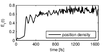
Figure 7 shows that the integrated difference $E_{1}(t)$ stays small only until $170$ fs and detoriates afterwards, illustrating the limitations of quasi-classical approximations as previously discussed in the literature[6, 23, 3]. By contrast, Figure 8 displays the much smaller deviation of the cumulative distribution functions $E_{c}(t)$ , which stays below $\sqrt{\varepsilon}\approx 0.11$ also for longer times, see §III.1 and Appendix C.

V.2 Henon–Heiles dynamics in higher dimensions

We present computations with confined Henon–Heiles potentials[24, 25] in dimensions $2$ to $32$ which illustrate the performance of the quasi-classical algorithm in moderately high-dimensional situations. Henon–Heiles systems have been previously simulated by different methods as the multiconfiguration time-dependent Hartree method (MCTDH)[24, 25, 26], semiclassical initial value representations[27, 28, 3] and coupled coherent states[29]. These studies have mostly aimed at the autocorrelation function $c_{t}=\langle\psi\mid U_{t}\mid\psi\rangle$ and its Fourier transform. For quasi-classical approximations only the modulus

(c_{t}^{*}c_{t})^{1/2}=\left(\left\langle U_{t}\psi\mid\psi\right\rangle\left\langle\psi\mid U_{t}\psi\right\rangle\right)^{1/2}

and not the complex number $c_{t}$ is computable.

V.2.1 The model system

We investigate the dynamics of a hydrogen atom on a $d$ -dimensional PES represented by the Henon–Heiles potential

\frac{m\omega^{2}}{2}\sum_{j=1}^{d}q_{j}^{2}+\sigma\sum_{j=1}^{d-1}(q_{j}^{2}q_{j+1}-\tfrac{1}{3}q_{j+1}^{2})

with[26] $m=1837m_{e}$ , $\sigma=0.0072E_{h}a_{0}^{-3}$ , and $m\omega^{2}=0.0248m_{e}({\rm a.t.u.})^{-2}$ . Rescaling space according to $q\mapsto q/\overline{q}=\sqrt{0.0248}\,q$ , we obtain the Schrödinger operator in semiclassical scaling

	$\displaystyle\widehat{H}=$
			$\displaystyle-\tfrac{\varepsilon^{2}}{2}\Delta+\tfrac{1}{2}\sum_{j=1}^{d}q_{j}^{2}+1.8436\sum_{j=1}^{d-1}(q_{j}^{2}q_{j+1}-\tfrac{1}{3}q_{j+1}^{2})$

with $\varepsilon=0.0037$ . Due to the large coupling constant $1.8436$ , the MCTDH calculations[26] for this Hamiltonian have employed complex absorbing potentials. Following Refs.[24, 25], we do not add a complex absorber but a quartic confinement that prevents phase space trajectories from escaping to infinity. Our modified Henon-Heiles potential reads

	$\displaystyle V_{d}(q)=$	$\displaystyle\tfrac{1}{2}\sum_{j=1}^{d}q_{j}^{2}+1.8436\sum_{j=1}^{d-1}(q_{j}^{2}q_{j+1}-\tfrac{1}{3}q_{j+1}^{2})$
		$\displaystyle+0.4\sum_{j=1}^{d-1}(q_{j}^{2}+q_{j+1}^{2})^{2}.$		(17)

As considered previously[26], we investigate as initial data (A) the shifted harmonic ground state (3) of width $\Sigma={\rm Id}$ , with initial position $q_{0,k}=0.0408$ nm and initial momentum $p_{0,k}=0$ for all $k=1,\ldots,d$ . In the rescaled units, the shift equals $q_{0,k}\approx 0.1215\overline{q}$ . This choice leads to an almost periodic evolution of the expected positions, see Figure 9. We contrast this setup by computations for Gaussian initial data (B) localized in $q_{0,k}=0.3645\overline{q}$ for all $k=1,\ldots,d$ . Showing a ball of wool for the position expectations, Figure 9 proves that the dynamics for these higher energy wave functions are less regular.

For both initial conditions, the total energy of the system grows with the dimension.

V.2.2 The numerical setup

In dimension $d=2$ , we compare the approximative expectation values of the kinetic, potential, and total energies obtained from the quasi-classical algorithm with reference data from a high resolution Strang splitting for the corresponding Schrödinger equation, see Table 2.

space area	Fourier modes	time	timesteps
$[-5,5]\times[-5,5]$	$2048\times 2048$	$[0,50]$	$5\cdot 10^{5}$

Table 2: Data of the reference solution of the vibrational Schrödinger equation for the

2

-dimensional Henon-Heiles system, generated by a split step Fourier solver on the time interval

[0,327{\rm fs}]

Because of the time rescaling, the final time of $50/\varepsilon$ atomic time units equals $327$ fs. In dimensions $d>2$ we restrict ourselves to the comparison of the evolution of potential energies, the preservation of the total energy and the computational effort.

For all classical trajectories, we used an symplectic integrator[19] of order $8$ with time stepping $\tau=10^{-1}$ .

V.2.3 Energy expectation values

Figure 10 shows the error of the quasi-classically computed expectation values of the total, potential and kinetic energy in dimension $d=2$ with $2^{11}$ Sobol points. The errors are small but larger than the ones obtained for the iodine system in Figure 3 and differ for the two initial data on the long time scale of the simulation. In particular, initial state (B) leads to less stable classical dynamics and a much faster local growth of errors than state (A).

In Figure 11, we present the time-evolution of the potential energy in dimensions $d=2,\ldots,32$ up to the shorter time $104\text{fs}$ where we used $2^{12}$ Sobol points for each of the calculations. The results show highly regular oscillations for setup (A), and slightly damped dynamics in the case of initial data (B).

Also the total energy deviation in Figure 12 has regular oscillations, which are bounded by $8\cdot 10^{-8}$ as expected for a symplectic eighth order time discretization with step size $\tau=10^{-1}$ . We note, that the results for a Monte Carlo sampling with $2^{14}$ normally distributed points and those for a Quasi-Monte Carlo sampling with $2^{12}$ Sobol points of the initial Wigner function are almost indistinguishable.

The computational times grow moderately with the dimension, reaching less than 20 seconds for the 32-dimensional case, see Table 3.

$d$	2	4	6	10	14	18	32
comp. time	0.7s	1.3s	2.0s	5.9s	7.7s	9.7s	19.8s

Table 3: Computational time (in seconds) for the propagation of

N=2^{12}

Sobol points for the

d

-dimensional Henon-Heiles system up to

104\text{fs}

V.2.4 Bath energy

Lastly, we revisit the dynamics for the $32$ -dimensional potential with slightly different initial data. As in Ref.[26], we view the last but four coordinates $q_{5},\ldots,q_{32}$ as bath degrees of freedom, and use the initial harmonic ground state with displacement $q_{0,k}\approx 0.1215\overline{q}$ only for the system coordinates $k=1,\ldots,4$ , while the bath degrees of freedom are localized at the origin.

We are interested in the evolution of the expectation value of the bath energy

	$\displaystyle\widehat{H_{B}}=$	$\displaystyle\tfrac{1}{2}\sum_{j=5}^{32}(-\varepsilon^{2}\partial_{q_{j}}^{2}+q_{j}^{2})+0.9218q_{4}^{2}q_{5}$
		$\displaystyle+1.8436\sum_{j=5}^{31}(q_{j}^{2}q_{j+1}-\tfrac{1}{3}q_{j+1}^{2}),$		(18)

where the bath coupling term $1.8436q_{4}^{2}q_{5}$ has been divided equally between the system and the bath Hamiltonian. The quartic confinement or rather the missing complex absorbing potential in $V_{32}$ does not allow for a quantitative comparison of the results in Figure 13 with the MCTDH calculations[26]. Nevertheless, the qualitative structure and the range of the dynamics agree well. The bath energy computation for Figure 13 used $2^{12}$ Sobol points and took $63$ seconds.

VI Conclusion

We have related quasi-classical approximation schemes as the linearized semiclassical initial value representation (LSC-IVR) and the Wigner phase space method to Egorov’s theorem. Depending on the quantity of interest, the error estimates may depend on the initial data: For the computation of typical expectation values, only normalized initial wave functions with $\langle\psi|\psi\rangle=1$ are required for an error of the order $\varepsilon^{2}$ . For the computation of position densities and transition probabilities, however, higher order derivatives of the inital Wigner function influence the accuracy of the approximation, such that for localized initial data the accuracy drops down to $\sqrt{\varepsilon}$ .

Our numerical experiments for a Morse model of diatomic iodine and for confined Henon–Heiles systems in various dimensions have illustrated the theoretical results but have also shown persistence on longer time scales than expected. The computational times are in the range of seconds.

The numerical computation of the approximation error’s proportionality factor $E(V,B,\Phi_{t})$ can be achieved by ordinary differential equations involving higher order derivatives of the potential $V$ and the observable $B$ . So far, these factors have successfully been computed for two-dimensional torsional dynamics[30], and the application to more demanding test systems seems to be a natural continuation of the research presented here.

VII Acknowledgments

This research was supported by the German Research Foundation (DFG), Collaborative Research Center SFB-TRR 109, and the graduate program TopMath of the Elite Network of Bavaria.

Appendix A Proof of Egorov’s theorem

Egorov’s theorem has a simple proof[13], whose key element is the asymptotic expansion of the commutator of Weyl quantized observables in even powers of $\varepsilon$ ,

	$\displaystyle\frac{i}{\varepsilon}\!\left[\widehat{A},\widehat{B}\right]$	$\displaystyle=$	$\displaystyle\frac{i}{\varepsilon}\!\left(\widehat{A}\widehat{B}-\widehat{B}\widehat{A}\right)$
		$\displaystyle\sim$	$\displaystyle\sum_{k=0}^{\infty}\left(\frac{\varepsilon}{2i}\right)^{2k}\widehat{\{A,B\}}_{2k+1},$

where the $k$ th order Poisson bracket is defined according to

\{A,B\}_{k}=\sum_{|\alpha+\beta|=k}\frac{(-1)^{|\beta|}}{\alpha!\beta!}\left(\partial_{q}^{\alpha}\partial_{p}^{\beta}B\right)\left(\partial_{q}^{\beta}\partial_{p}^{\alpha}A\right).

One argues as follows:

$\displaystyle U_{-t}\,\widehat{B}\,U_{t}-\widehat{B\circ\Phi_{t}}$
	$\displaystyle=$	$\displaystyle\int_{0}^{t}\frac{d}{ds}\left(U_{-s}\widehat{B\circ\Phi}_{t-s}U_{s}\right)ds$
	$\displaystyle=$	$\displaystyle\int_{0}^{t}U_{-s}\left(\tfrac{i}{\varepsilon}[\widehat{H},\widehat{B\circ\Phi}_{t-s}]-\partial_{t}\widehat{B\circ\Phi}_{t-s}\right)U_{s}ds$
	$\displaystyle\sim$	$\displaystyle\sum_{k=1}^{\infty}\left(\frac{\varepsilon}{2i}\right)^{2k}\int_{0}^{t}U_{-s}\,{\rm op}({\{H,B\circ\Phi_{t-s}\}}_{2k+1})U_{s}\,ds,$

with ${\rm op}(A)=\widehat{A}$ , since

\partial_{t}(B\circ\Phi_{t-s})=\{H,B\circ\Phi_{t-s}\}_{1}.

The second order term

-\frac{\varepsilon^{2}}{4}\int_{0}^{t}U_{-s}\,{\rm op}(\{H,B\circ\Phi_{t-s}\}_{3})\,U_{s}\,ds

is expected to dominate the approximation error $E(V,B,\Phi_{t})$ in Egorov’s theorem (6).

Appendix B Approximating position densities

In contrast to the LSC-IVR approximation error, which is uniform over all initial states with $\langle\psi\mid\psi\rangle=1$ , the accuracy of the quasi-classical computation of position densities[16] by a combination of Egorov’s theorem with the Fourier inversion formula depends on the initial state: The error of (8) is

\varepsilon^{2}\langle\psi\mid\int E(V,B_{\eta},\Phi_{t})d\eta\mid\psi\rangle.

The dominant part of this term contains third order derivatives of the potential $V$ and the observable $B_{\eta}$ , that is,

$\displaystyle\int_{0}^{t}\int\langle U_{s}\psi\mid{\rm op}(\partial_{q}^{3}V\partial_{p}^{3}(B_{\eta}\circ\Phi_{t-s})\mid U_{s}\psi\rangle d\eta ds$
	$\displaystyle=$	$\displaystyle\int_{0}^{t}\int W_{s}(z)\,\partial_{q}^{3}V(q)\,\partial_{p}^{3}(e^{-i\eta\cdot(q_{t-s}-r)})dzd\eta ds$
	$\displaystyle=$	$\displaystyle-\int_{0}^{t}\int(\partial_{p}^{3}W_{s})(\Phi_{s-t}(z))\,(\partial_{q}^{3}V)(q_{s-t})$
		$\displaystyle\qquad\qquad e^{-i\eta\cdot(q-r)}dzd\eta ds,$

where $W_{s}$ denotes the Wigner function of the time-evolved wave function $U_{s}\psi$ . This implies, that the error is not uniform over all initial wave functions $\psi$ with $\langle\psi|\psi\rangle=1$ , but crucially depends on third derivatives of its time-evolved Wigner function.

Appendix C Heuristics for Wigner derivatives

We present a heuristic argument, explaining the considerable difference between the integrated error measure $E_{1}(t)$ and the cumulative measure $E_{c}(t)$ proposed in §V.1.4.

If the initial state $\psi$ is a vibrational Gaussian wavepacket (3), then there are $\Sigma$ -dependent complex numbers $c_{m,n}$ such that

\partial_{p}^{3}W_{\psi}=\varepsilon^{-3/2}\sum_{|(m,n)|\leq 3}c_{m,n}\,W(\psi_{m},\psi_{n}),

where

	$\displaystyle W(\psi_{m},\psi_{n})(q,p)=$
			$\displaystyle(2\pi\varepsilon)^{-d}\int\psi_{m}(q-\tfrac{1}{2}y)\psi_{n}^{*}(q+\tfrac{1}{2}y)e^{ip\cdot y/\varepsilon}dy$

denotes the joint Wigner function of two generalized coherent states[31, 14] $\psi_{m}$ and $\psi_{n}$ . We approximate

	$\displaystyle(\partial_{p}^{3}W_{s})(\Phi_{s-t})(z)\approx$
			$\displaystyle\varepsilon^{-3/2}\sum_{\|(m,n)\|\leq 3}c_{m,n}\,W(U_{t}\psi_{m},U_{t}\psi_{n})$

and obtain

	$\displaystyle\|(U_{t}\psi)(r)\|^{2}-P_{t}(r)\approx$
			$\displaystyle\sqrt{\varepsilon}\,F(V,\Phi_{t})\sum_{\|(m,n)\|\leq 3}(U_{t}\psi_{m})(r)\,(U_{t}\psi_{n})(r)^{*},$

where $F(V,\Phi_{t})$ depends on the potential $V$ and the flow $\Phi_{t}$ . This implies for the two error measures

	$\displaystyle E_{1}(t)\approx\sqrt{\varepsilon}\,\|F(V,\Phi_{t})\|$
			$\displaystyle\int_{0}^{\infty}\Big\|\sum_{\|(m,n)\|\geq 3}(U_{t}\psi_{m})(r)\,(U_{t}\psi_{n})(r)^{*}\Big\|dr$

and

	$\displaystyle E_{c}(t)\approx\sqrt{\varepsilon}\,\|F(V,\Phi_{t})\|$
			$\displaystyle\sup_{x\geq 0}\Big\|\sum_{\|(m,n)\|\leq 3}\int_{0}^{x}(U_{t}\psi_{m})(r)\,(U_{t}\psi_{n})(r)^{*}dr\Big\|.$

The decisive difference between the two error measures is therefore, that $E_{1}(t)$ depends on the integrated modulus of products of excited coherent states, whereas $E_{c}(t)$ sees the modulus of their cumulative overlap.

References

[1] W. Miller, J. Chem. Phys. 61, 1823 (1974).
[2] H. Wang, X. Sun, and W. Miller, J. Chem. Phys. 108, 9726 (1998).
[3] M. Thoss and H. Wang, Ann. Rev. Phys. Chem. 55, 299 (2004).
[4] E. J. Heller, J. Chem. Phys. 65, 1289 (1976).
[5] R. Brown and E. Heller, J. Chem. Phys. 75, 186 (1981).
[6] M. Davis and E. Heller, J. Chem. Phys. 80, 5036 (1984).
[7] H. Lee and M. Scully, J. Chem. Phys. 73, 2238 (1980).
[8] X. Sun, H. Wang, and W. Miller, J. Chem. Phys. 109, 4190 (1998).
[9] S. Habershon and D. Manolopoulos, J. Chem. Phys. 131, 244518 (2009).
[10] Q. Shi and E. Geva, J. Chem. Phys. 118, 8173 (2003).
[11] J. Poulsen and P. Nyman, G Rossky, J. Chem. Phys. 119, 12179 (2003).
[12] Y. Egorov, Uspekhi Mat. Nauk 24, 235 (1969).
[13] A. Bouzouina and D. Robert, Duke Math. J. 111, 223 (2002).
[14] C. Lasser and S. Troppmann, J. Fourier An. Appl., 1(2014).
[15] C. Lasser and S. Röblitz, SIAM J. Sci. Comput. 32, 1465 (2010).
[16] X. Sun and W. Miller, J. Chem. Phys. 110, 6635 (1999).
[17] S. Kube, C. Lasser, and M. Weber, J. Comput. Phys. 228, 1947 (2009).
[18] J. Keller and C. Lasser, SIAM J. Appl. Math. 73, 1557 (2013).
[19] H. Yoshida, Phys. Lett. A 150, 262 (1990).
[20] E. Hairer, C. Lubich, and G. Wanner, Geometric numerical integration (Springer, Heidelberg, 2010).
[21] R. F. Barrow and K. K. Yee, J. Chem. Soc., Faraday Trans. 2 69, 684 (1973).
[22] J.-Y. Fang and C. C. Martens, J. Chem. Phys. 105, 9072 (1996).
[23] H. Wang, M. Thoss, K. L. Sorge, R. Gelabert, X. Gimenez, and W. H. Miller, J. Chem. Phys. 114, 2562 (2001).
[24] H.-D. Meyer, U. Manthe, and L. Cederbaum, Chem. Phys. Lett. 165, 73 (1990), ISSN 0009-2614.
[25] A. Raab and H.-D. Meyer, J. Chem. Phys. 112, 10718 (2000).
[26] M. Nest and H.-D. Meyer, J. Chem. Phys. 117, 10499 (2002).
[27] M. Brewer, J. Chem. Phys. 111, 6168 (1999).
[28] H. Wang, D. E. Manolopoulos, and W. H. Miller, J. Chem. Phys. 115, 6317 (2001).
[29] D. Shalashilin and M. Child, Chem. Phys. 304, 103 (2004).
[30] W. Gaim and C. Lasser arXiv:1403.2839 [math-na].
[31] G. Hagedorn, Ann. Phys. 269, 77 (1998).