跳到论文正文
W Papers独立论文阅读器 arXiv:1405.7244 论文正文 计算阅读时间 · 0%
引用这篇论文根据当前论文元数据生成,正式投稿前建议核对。


License: arXiv.org perpetual non-exclusive license
arXiv:1405.7244v3 [math.ST] 11 Mar 2015

L2L^{2} Asymptotics for High-Dimensional Data

Mengyu Xu, Danna Zhang and Wei Biao Wu

Department of Statistics
University of Chicago
5734 S. University Avenue
Chicago, Illinois 60637
USA

November 24, 2014

Abstract

We develop an asymptotic theory for L2L^{2} norms of sample mean vectors of high-dimensional data. An invariance principle for the L2L^{2} norms is derived under conditions that involve a delicate interplay between the dimension pp, the sample size nn and the moment condition. Under proper normalization, central and non-central limit theorems are obtained. To facilitate the related statistical inference, we propose a plug-in calibration method and a re-sampling procedure to approximate the distributions of the L2L^{2} norms. Our results are applied to multiple tests and inference of covariance matrix structures.

MSC Subject Classifications (2010): 62G20, 62H15, 62G10.
Key words and phrases: L2L^{2} asymptotics, Gaussian approximation, invariance principle, large pp small nn, multiple testing.

1 Introduction

Let X,Xi,i∈ℤ,X,X_{i},i\in\mathbb{Z}, be independent and identically distributed (i.i.d.) pp-dimensional random vectors with mean 𝔼​Xi=μ\mathbb{E}X_{i}=\mathbf{\mu} and covariance matrix cov⁡(Xi)=Σ\mathrm{cov}(X_{i})=\Sigma. Given the sample X1,…,XnX_{1},\ldots,X_{n}, we can estimate the mean μ\mathbf{\mu} by the sample mean X¯n=∑i=1nXi/n\bar{X}_{n}=\sum_{i=1}^{n}X_{i}/n. The primary goal of the paper concerns the asymptotic distribution of |X¯n−μ|2=(X¯n−μ)T​(X¯n−μ)|\bar{X}_{n}-\mathbf{\mu}|^{2}=(\bar{X}_{n}-\mathbf{\mu})^{T}(\bar{X}_{n}-\mathbf{\mu}). The latter problem has a range of important applications in statistics including multiple tests and inference of covariance structures. Unless otherwise specified, assume throughout the paper that μ=0\mathbf{\mu}=0.

In the classical setting with fixed dimension pp, due to the Central Limit Theorem, we have n​X¯n⇒N⁡(0,Σ)\sqrt{n}\bar{X}_{n}\Rightarrow N(0,\Sigma). Hence, letting Y∼N⁡(0,Σ)Y\sim N(0,\Sigma), we have by Slutsky’s Theorem that

supu∈ℝ|ℙ⁡(n​X¯nT​X¯n≤u)−ℙ⁡(YT​Y≤u)|→0.\displaystyle\sup_{u\in\mathbb{R}}|\mathbb{P}(n\bar{X}_{n}^{T}\bar{X}_{n}\leq u)-\mathbb{P}(Y^{T}Y\leq u)|\to 0. (1.1)

In this paper we shall discuss the validity of (1.1) in situations in which pp can be unbounded. In modern problems, the dimension pp can be larger than the sample size nn. In this case, the traditional methods may not work. For example, Portnoy [34] showed that the CLT is generally no longer valid when pp is large such that n=o⁡(p)\sqrt{n}=o(p). For other contributions see Bentkus [5], Bentkus [6]. Thus different methods are needed to prove (1.1). The latter problem in the high dimensional setting and the corresponding statistical inference issues are challenging and have attracted wide attention. For linear processes, by Bai and Saranadasa [2], one can prove that n​X¯nT​X¯n−tr⁡(𝐗n​𝐗nT)/nn\bar{X}_{n}^{T}\bar{X}_{n}-\mathrm{tr}(\mathbf{X}_{n}\mathbf{X}^{T}_{n})/n, where 𝐗n=(X1,…,Xn)\mathbf{X}_{n}=(X_{1},\ldots,X_{n}) is the data matrix, is asymptotically Gaussian, assuming that p/np/n tends to a finite constant and the largest eigenvalue of Σ\Sigma is negligible relative to its Frobenius norm. The latter condition can be violated in cases such as factor models, as discussed in Katayama et al. [27], who studied the asymptotic distribution of ZT​Z−tr⁡(Σ)Z^{T}Z-\mathrm{tr}(\Sigma) over different types of Σ\Sigma under Z∼N⁡(0,Σ)Z\sim N(0,\Sigma).

In this paper, we shall develop an asymptotic theory for X¯nT​X¯n\bar{X}_{n}^{T}\bar{X}_{n} for a generally distributed XX, without requiring normality or linearity assumption. In particular, we shall apply the normal comparison method of Stein type and show that X¯nT​X¯n\bar{X}_{n}^{T}\bar{X}_{n} can be approximated by a mixture of independent χ2\chi^{2} distributions. The approximate distribution may or may not be asymptotically normal. Specifically, we shall establish the following equivalent form of (1.1):

supu∈ℝ|ℙ⁡(n​X¯nT​X¯n≤u)−ℙ⁡(n​Y¯nT​Y¯n≤u)|→0,\displaystyle\sup_{u\in\mathbb{R}}|\mathbb{P}(n\bar{X}_{n}^{T}\bar{X}_{n}\leq u)-\mathbb{P}(n\bar{Y}_{n}^{T}\bar{Y}_{n}\leq u)|\to 0, (1.2)

where Yi,i∈ℤ,Y_{i},i\in\mathbb{Z}, are i.i.d. N⁡(0,Σ)N(0,\Sigma) random vectors and Y¯n=∑i=1nYi/n\bar{Y}_{n}=\sum_{i=1}^{n}Y_{i}/n. We can view (1.2) as an invariance principle in a general sense since the distributions of functions of non-Gaussian random vectors can be approximated by those of Gaussian vectors with the same covariance structure. The invariance principle in the narrow sense refers to the Gaussian approximation of partial sum processes of non-Gaussian random variables; cf Berkes et al. [7].

As an immediate application of (1.1) or (1.2), one can perform the multiple test for the hypothesis

H0:μ=μ0\displaystyle H_{0}:\mu=\mu_{0} (1.3)

for some pre-specified vector μ0\mu_{0}. Assume without loss of generality that μ0=0\mu_{0}=0. A classical approach is to use the Hotelling T2T^{2} statistic

Tn=n​X¯nT​Σ^n−1​X¯n,\displaystyle T_{n}=n\bar{X}_{n}^{T}\hat{\Sigma}_{n}^{-1}\bar{X}_{n}, (1.4)

where Σ^n=(n−1)−1​∑i=1n(Xi−X¯n)​(Xi−X¯n)T\hat{\Sigma}_{n}=(n-1)^{-1}\sum_{i=1}^{n}(X_{i}-\bar{X}_{n})(X_{i}-\bar{X}_{n})^{T} is the sample covariance matrix. In the high dimensional setting with p>np>n, Σ^n\hat{\Sigma}_{n} is singular and then TnT_{n} is not well-defined. Bai and Saranadasa [2] pointed out that this test lacks power. There is a large literature accommodating the Hotelling T2T^{2} type statistic into the high-dimensional situation; see for example, Dempster [16], Dempster [17], Bai and Saranadasa [2], Chen and Qin [12], Srivastava et al. [43], among others. Dempster [16], Dempster [17], Srivastava et al. [43] considered Gaussian vectors. For the non-Gaussian random vectors, existing works assume linear forms. Central limit theorems for quadratic forms of sample mean vectors were proved in Bai and Saranadasa [2], Chen and Qin [12], Katayama and Kano [26].

We test the hypothesis H0H_{0} by directly using the test statistic n​X¯nT​X¯nn\bar{X}_{n}^{T}\bar{X}_{n}. Given the significance level α∈(0,1)\alpha\in(0,1), let u1−αu_{1-\alpha} be the (1−α)(1-\alpha)th quantile of YT​YY^{T}Y. Namely ℙ⁡(YT​Y≤u1−α)=1−α\mathbb{P}(Y^{T}Y\leq u_{1-\alpha})=1-\alpha. Then H0H_{0} is rejected if n​X¯nT​X¯n>u1−αn\bar{X}_{n}^{T}\bar{X}_{n}>u_{1-\alpha}. By (1.1), the latter test has an asymptotic level α\alpha.

If Σ\Sigma is known, the cutoff value u1−αu_{1-\alpha} can be easily computed, either numerically or analytically, since the distribution of YT​YY^{T}Y is completely known. In most applications, however, Σ\Sigma is not known. We consider two approaches. The first one is to use an estimate of Σ\Sigma. With the estimated covariance matrix, we can simulate a cutoff value. To access the goodness of the cutoff value with estimated covariance matrices, we shall introduce a new matrix convergence criterion: the normalized consistency. It is closely related, but different from the widely used spectral norm convergence. From modern random matrix theory, it is now well-known that the sample covariance matrix Σn\Sigma_{n} is not a (spectral norm) consistent estimator of Σ\Sigma when pp is large; see Marčenko and Pastur [31], Bai and Silverstein [3], Wachter [45], Geman [21], Yin et al. [49], Johnstone [25], El Karoui [18], to name a few. However, our results indicate that the sample covariance matrix can be normalized consistent in spectral norm, and hence the corresponding estimated cutoff value is consistent. The normalized consistency guarantees the validity of resampling procedures. Details are given in Section 3.1. As our second approach, we use the subsampling technique, which avoids estimating Σ\Sigma or its eigenvalues; see Section 3.2.

Another type of approach for testing (1.3) is to use the maximum or L∞L^{\infty} norm |X¯n|∞=maxj≤p⁡|X¯n​j||\bar{X}_{n}|_{\infty}=\max_{j\leq p}|{\bar{X}}_{nj}| or the studentized version maxj≤p⁡|X¯n​j|/σ^j\max_{j\leq p}|{\bar{X}}_{nj}|/\hat{\sigma}_{j}, where σ^j2\hat{\sigma}_{j}^{2} are estimates for the marginal variances σj2=var⁡(Xi​j)\sigma_{j}^{2}={\rm var}(X_{ij}). Kosorok and Ma [28] considered the uniform consistency problem, and Fan et al. [19] performed the L∞L^{\infty} test via Bonferroni correction, thus completely ignoring dependencies between entries of XiX_{i}. In a recent work, Chernozhukov et al. [14] derived a Gaussian approximation for |X¯n|∞|\bar{X}_{n}|_{\infty} in the high-dimensional setting. In comparison with the marginal testing procedures, the procedure in Chernozhukov et al. [14] is dependence-adjusted. Liu and Shao [30] established a deep Carmér-type moderate deviation principle for Hotelling’s T2T^{2} statistic under mild moment condition. The L2L^{2}-based test can be more powerful if the alternative consists of many small but non-zero signals that are of similar magnitudes.

This paper is organized as follows. In Section 2, we present the Gaussian approximation result. Section 3 provides a plug-in calibration of the Gaussian analogue when Σ\Sigma is unknown. We introduce normalized consistency, a new matrix convergence criterion. A sub-sampling procedure is also introduced there. In Section 4 we apply our result to the mean inference problem for linear processes. Section 5 deals with the covariance matrix structure inference for linear processes. Proofs are given in Sections 7.

We now introduce some notation. For a vector 𝐱=(x1,…,xm)T\mathbf{x}=(x_{1},\ldots,x_{m})^{T}, let the length |𝐱|=|𝐱|2=(𝐱T​𝐱)1/2|\mathbf{x}|=|\mathbf{x}|_{2}=(\mathbf{x}^{T}\mathbf{x})^{1/2}. Here 𝐱T​𝐱=∑i=1mxi2\mathbf{x}^{T}\mathbf{x}=\sum_{i=1}^{m}x_{i}^{2}. Let XX be a random vector. Write X∈ℒqX\in{\cal L}^{q}, q>0q>0, if ‖X‖q:=(𝔼​|X|q)1/q<∞\left\|X\right\|_{q}:=(\mathbb{E}|X|^{q})^{1/q}<\infty. For a matrix A=(aj​k)j,kA=(a_{jk})_{j,k}, ρ⁡(A)=max𝐱⁡|A​𝐱|/|𝐱|\rho(A)=\max_{\mathbf{x}}|A\mathbf{x}|/|\mathbf{x}| (resp. |A|F=(∑j​kaj​k2)1/2\left|A\right|_{F}=(\sum_{jk}a_{jk}^{2})^{1/2}) denotes its spectral (resp. Frobenius) norm. Write the p×pp\times p identity matrix as Idp{\rm Id}_{p}. Denote by CC a positive constant whose value may vary from place to place.

2 Main Result

Consider i.i.d. random vectors X,Xi∈ℝpX,X_{i}\in\mathbb{R}^{p}, i∈ℤi\in\mathbb{Z}, with 𝔼​Xi=0\mathbb{E}X_{i}=0 and covariance matrix cov⁡(Xi)=Σ\mathrm{cov}(X_{i})=\Sigma. Let Σ=Q​Λ​QT\Sigma=Q\Lambda Q^{T} be its eigen-decomposition, where QQ is an orthonormal matrix with QT​Q=IdpQ^{T}Q={\rm Id}_{p} and Λ=diag⁡(λ1,…,λp)\Lambda=\mathrm{diag}\left(\lambda_{1},\ldots,\lambda_{p}\right), with λ1≥…≥λp≥0\lambda_{1}\geq\ldots\geq\lambda_{p}\geq 0. Given data X1,…,XnX_{1},\ldots,X_{n}, let Σ^=n−1​𝐗n​𝐗nT\hat{\Sigma}=n^{-1}\mathbf{X}_{n}\mathbf{X}_{n}^{T}, where 𝐗n=(X1,…,Xn)\mathbf{X}_{n}=(X_{1},\ldots,X_{n}), be the sample covariance matrix; let λ^1≥…≥λ^p≥0\hat{\lambda}_{1}\geq\ldots\geq\hat{\lambda}_{p}\geq 0 be the eigenvalues of Σ^\hat{\Sigma}. Define

fk:=[tr(Σk)]1/k and f^k:=[tr(Σ^k)]1/k,k=1,2,….\displaystyle f_{k}:=[\mathrm{tr}(\Sigma^{k})]^{1/k}\mbox{ and }\hat{f}_{k}:=[\mathrm{tr}(\hat{\Sigma}^{k})]^{1/k},\quad k=1,2,\ldots.

Then fkk=∑i=1pλikf_{k}^{k}=\sum_{i=1}^{p}\lambda_{i}^{k} and f^kk=∑i=1pλ^ik\hat{f}_{k}^{k}=\sum_{i=1}^{p}\hat{\lambda}_{i}^{k}. For the Frobenius norm with k=2k=2, we simply write f=f2f=f_{2} and f^=f^2\hat{f}=\hat{f}_{2}.

Our main result is Theorem 2.2 which asserts that under suitable conditions the distributions of quadratic functions of X¯nT​X¯n\bar{X}_{n}^{T}\bar{X}_{n} and Y¯nT​Y¯n\bar{Y}_{n}^{T}\bar{Y}_{n} are asymptotically close. In our asymptotic relation, we let n→∞n\to\infty and view the dimension p=pnp=p_{n} which satisfies pn→∞p_{n}\to\infty as n→∞n\to\infty. To state the theorem, we need to impose the following condition on XX.

Condition 1.

Let δ>0\delta>0. Assume that

Kδ​(X)2+δ:=𝔼​||X1|22−f1f|2+δ\displaystyle K_{\delta}(X)^{2+\delta}:=\mathbb{E}\left|{\left|X_{1}\right|_{2}^{2}-f_{1}\over f}\right|^{2+\delta} <∞;\displaystyle<\infty; (2.1)
Dδ​(X)2+δ:=𝔼​|X1T​X2f|2+δ\displaystyle D_{\delta}(X)^{2+\delta}:=\mathbb{E}\left|{{X_{1}^{T}X_{2}}\over f}\right|^{2+\delta} <∞.\displaystyle<\infty. (2.2)

In conditions (2.1) and (2.2), Kδ​(X)K_{\delta}(X) and Dδ​(X)D_{\delta}(X) depend on the distribution of XX. In the sequel for notational convenience we abbreviate them as KδK_{\delta} and DδD_{\delta}, respectively. Note that D0=1D_{0}=1. In Sections 4 and 5 we shall bound KδK_{\delta} and DδD_{\delta} for mean and covariance matrix inference problems arising from linear processes. Remark 2.5 provides an upper bound for moments of sums of dependent random variables using Rosenblatt transforms. Proposition 2.1 shows that for Gaussian vectors we can have explicit upper bounds.

Proposition 2.1.

Let YiY_{i} be i.i.d. N⁡(𝟎,Σ)N(\mathbf{0},\Sigma) and δ≥0\delta\geq 0. Then

𝔼​||Y1|22−f1f|2+δ\displaystyle\mathbb{E}\left|{\left|Y_{1}\right|_{2}^{2}-f_{1}\over f}\right|^{2+\delta} ≤cδ2+δ;\displaystyle\leq c_{\delta}^{2+\delta}; (2.3)
𝔼​|Y1T​Y2f|2+δ\displaystyle\mathbb{E}\left|{Y_{1}^{T}Y_{2}\over f}\right|^{2+\delta} ≤dδ2+δ,\displaystyle\leq d_{\delta}^{2+\delta}, (2.4)

where cδ=(1+δ)1/2​‖ξ2−1‖2+δc_{\delta}=(1+\delta)^{1/2}\|\xi^{2}-1\|_{2+\delta}, dδ=(1+δ)1/2​‖ξ‖2+δ2d_{\delta}=(1+\delta)^{1/2}\|\xi\|^{2}_{2+\delta} and ξ∼N⁡(0,1)\xi\sim N(0,1).

Based on (2.1) and (2.2), we have the following asymptotic result. Let ηi,i∈ℤ,\eta_{i},i\in\mathbb{Z}, be i.i.d. χ12\chi^{2}_{1} random variables. Consider the normalized version

Rn=n​|X¯n|22−f1f.\displaystyle R_{n}={{n|\bar{X}_{n}|_{2}^{2}-f_{1}}\over f}. (2.5)
Theorem 2.2.

Assume that (2.1) and (2.2) hold with 0<δ≤10<\delta\leq 1. Then

supt|ℙ(Rn≤t)−ℙ(V≤t)|=O(ψn−1/2), where V=∑j=1pλjf(ηj−1).\displaystyle\sup_{t}\left|\mathbb{P}\left(R_{n}\leq t\right)-\mathbb{P}\left(V\leq t\right)\right|=O(\psi_{n}^{-1/2}),\mbox{ where }V=\sum_{j=1}^{p}{{\lambda_{j}}\over f}(\eta_{j}-1). (2.6)

Here ψn\psi_{n} is the solution to the equation Lδ(n,ψ)=ψ−1/2L_{\delta}(n,\psi)=\psi^{-1/2} with

Lδ​(n,ψ)=ψ2​(K~02n+K~0n1/2)+ψq​[K~δqnq−1+𝔼​(X1T​Σ​X1)q/2nδ/2​fq+D~δqnδ],\displaystyle L_{\delta}(n,\psi)=\psi^{2}({\tilde{K}_{0}^{2}\over n}+{\tilde{K}_{0}\over n^{1/2}})+\psi^{q}[{\tilde{K}_{\delta}^{q}\over n^{q-1}}+{\mathbb{E}(X_{1}^{T}\Sigma X_{1})^{q/2}\over{n^{\delta/2}f^{q}}}+{\tilde{D}_{\delta}^{q}\over n^{\delta}}],

where q=2+δq=2+\delta, K~δ=Kδ+cδ\tilde{K}_{\delta}=K_{\delta}+c_{\delta}, D~δ=Dδ+dδ\tilde{D}_{\delta}=D_{\delta}+d_{\delta}, and cδc_{\delta} and dδd_{\delta} are given in Proposition 2.1. In particular, we have ψn→∞\psi_{n}\to\infty if

K~02n+K~δqnq−1+𝔼​(X1T​Σ​X1)q/2nδ/2​fq+D~δqnδ→0​ as ​n→∞.\displaystyle{\tilde{K}_{0}^{2}\over n}+{\tilde{K}_{\delta}^{q}\over n^{q-1}}+{\mathbb{E}(X_{1}^{T}\Sigma X_{1})^{q/2}\over{n^{\delta/2}f^{q}}}+{\tilde{D}_{\delta}^{q}\over n^{\delta}}\to 0\mbox{ as }n\to\infty. (2.7)

Consequently the left hand side of (2.6) converges to 00.

Note that 𝔼​(ηi−1)2=2\mathbb{E}(\eta_{i}-1)^{2}=2. By Lindeberg’s Central Limit Theorem,

V=∑j=1pf−1​λj​(ηj−1)⇒N⁡(0,2)\displaystyle V=\sum_{j=1}^{p}f^{-1}\lambda_{j}(\eta_{j}-1)\Rightarrow N(0,2)

holds if and only if λ1/f=ρ⁡(Σ)/f→0\lambda_{1}/f=\rho(\Sigma)/f\to 0. In this case by Theorem 2.2, RnR_{n} is also asymptotically N⁡(0,2)N(0,2). In the previous literature, the primary focus is on the asymptotic normality of X¯nT​X¯n\bar{X}_{n}^{T}\bar{X}_{n} or its modified version; see for example Bai and Saranadasa [2], Srivastava [42], Chen and Qin [12]. As an exception, Katayama et al. [27] considered situations in which the CLT fails. If λ1/f\lambda_{1}/f does not converge to 00, RnR_{n} may not have a Gaussian limit. When the dependence between entries of XX is strong, the asymptotic distribution of RnR_{n} can be non-normal. For example, suppose Y∼N⁡(0,Σ)Y\sim N(0,\Sigma) and Σ\Sigma is Toeplitz with diagonal 11 and σj,k∼|k−j|−D\sigma_{j,k}\sim|k-j|^{-D} for some 0<D<1/20<D<1/2 as |k−j|→∞|k-j|\to\infty. Then (YT​Y−f1)/f⇒∑j=1∞cj​(ηj−1)(Y^{T}Y-f_{1})/f\Rightarrow\sum_{j=1}^{\infty}c_{j}(\eta_{j}-1), the Rosenblatt distribution, with cj∼c​jD−1c_{j}\sim cj^{D-1} as j→∞j\to\infty, and cc is a constant; see Veillette and Taqqu [44].

Remark 2.3.

Since X1T​Σ​X1=𝔼⁡(X1T​X2​X2T​X1|X1)X_{1}^{T}\Sigma X_{1}=\mathbb{E}(X_{1}^{T}X_{2}X_{2}^{T}X_{1}|X_{1}), by Jensen’s inequality,

𝔼​(X1T​Σ​X1)q/2≤𝔼⁡(|X1T​X2​X2T​X1|q/2)=𝔼⁡(|X1T​X2|q)=Dδq​fq.\displaystyle\mathbb{E}(X_{1}^{T}\Sigma X_{1})^{q/2}\leq\mathbb{E}(|X_{1}^{T}X_{2}X_{2}^{T}X_{1}|^{q/2})=\mathbb{E}(|X_{1}^{T}X_{2}|^{q})=D_{\delta}^{q}f^{q}. (2.8)

So (2.7) follows from K~02/n+K~δq/nq−1+D~δq/nδ/2→0\tilde{K}_{0}^{2}/n+{\tilde{K}_{\delta}^{q}/n^{q-1}}+{\tilde{D}_{\delta}^{q}/n^{\delta/2}}\to 0 as n→∞n\to\infty. Namely if nn is sufficiently large such that K~02+K~δq/(q−1)+D~δ2​q/δ=o⁡(n)\tilde{K}_{0}^{2}+\tilde{K}_{\delta}^{q/(q-1)}+\tilde{D}_{\delta}^{2q/\delta}=o(n), then the left hand side of (2.6) holds with rate ψn−1/2→0\psi_{n}^{-1/2}\to 0. ∎

Remark 2.4.

If Conditions (2.1) and (2.2) hold with KδK_{\delta} and DδD_{\delta} bounded, then we can choose ψn≍nδ/(5+2​δ)\psi_{n}\asymp n^{\delta/(5+2\delta)} and the corresponding convergence rate in (2.6) is O(n−δ/(10+4δ))O(n^{-\delta/(10+4\delta)}). ∎

Remark 2.5.

Using the Rosenblatt transform ([36]), we can find measurable functions G1,…,GpG_{1},\ldots,G_{p} and i.i.d. standard uniform random variables U1,…,UpU_{1},\ldots,U_{p} such that X1X_{1} and the random vector (G1​(𝒰1),…,Gp​(𝒰p))T(G_{1}({\cal U}_{1}),\ldots,G_{p}({\cal U}_{p}))^{T} are identically distributed. Here 𝒰j=(U1,…,Uj){\cal U}_{j}=(U_{1},\ldots,U_{j}). Following Wu [46], define the predictive dependence measure θi,j,q=‖𝒫i​Gj2​(𝒰j)‖q\theta_{i,j,q}=\|{\cal P}_{i}G^{2}_{j}({\cal U}_{j})\|_{q}, where 𝒫i⋅=𝔼(⋅|𝒰i)−𝔼(⋅|𝒰i−1){\cal P}_{i}\cdot=\mathbb{E}(\cdot|{\cal U}_{i})-\mathbb{E}(\cdot|{\cal U}_{i-1}) is the projection operator. Since X1T​X1−f1=∑i=1p𝒫i​X1T​X1=∑i=1p∑j=ip𝒫i​Gj2​(𝒰j)X_{1}^{T}X_{1}-f_{1}=\sum_{i=1}^{p}{\cal P}_{i}X_{1}^{T}X_{1}=\sum_{i=1}^{p}\sum_{j=i}^{p}{\cal P}_{i}G^{2}_{j}({\cal U}_{j}), we have by Burkholder’s inequality (p. 396 in [15]) that

‖X1T​X1−f1‖q2q−1≤∑i=1p‖𝒫i​X1T​X1‖q2≤∑i=1p(∑j=ipθi,j,q)2.\displaystyle{{\|X_{1}^{T}X_{1}-f_{1}\|_{q}^{2}}\over{q-1}}\leq\sum_{i=1}^{p}\|{\cal P}_{i}X_{1}^{T}X_{1}\|_{q}^{2}\leq\sum_{i=1}^{p}\left(\sum_{j=i}^{p}\theta_{i,j,q}\right)^{2}.

A similar upper bound also holds for the LqL^{q} norm ‖X1T​X2‖q\|X_{1}^{T}X_{2}\|_{q}. ∎

To estimate the quantity |μ|22=μT​μ|\mu|_{2}^{2}=\mu^{T}\mu based on i.i.d. vectors X1,…,XnX_{1},\ldots,X_{n} with 𝔼​Xi=μ\mathbb{E}X_{i}=\mu, besides the natural plug-in estimator X¯nT​X¯n\bar{X}_{n}^{T}\bar{X}_{n}, we can also use the unbiased estimator (n⁡(n−1))−1​∑i≠j≤nXiT​Xj(n(n-1))^{-1}\sum_{i\not=j\leq n}X_{i}^{T}X_{j}; see also Chen and Qin [12]. This leads to the following variant of (2.5):

R~n=∑i≠j≤nXiT​Xj(n−1)​f\displaystyle\tilde{R}_{n}=\frac{\sum_{i\neq j\leq n}X_{i}^{T}X_{j}}{(n-1)f} (2.9)

Using the arguments in the proof of Theorem 2.2, without essential extra difficulties, we have the Gaussian approximation result:

Corollary 2.6.

Assume Condition (2.2) and μ=0\mu=0. Further assume

Lδ†:=𝔼​(X1T​Σ​X1)q/2nδ/2​fq+D~δqnδ→0.\displaystyle L^{\dagger}_{\delta}:={\mathbb{E}(X_{1}^{T}\Sigma X_{1})^{q/2}\over{n^{\delta/2}f^{q}}}+{\tilde{D}_{\delta}^{q}\over n^{\delta}}\to 0. (2.10)

Then ψn:=(Lδ†)−1/(q+1/2)→∞\psi_{n}:=(L^{\dagger}_{\delta})^{-1/(q+1/2)}\to\infty and, recall V=∑j=1pf−1​λj​(ηj−1)V=\sum_{j=1}^{p}f^{-1}\lambda_{j}(\eta_{j}-1),

supt|ℙ(R~n≤t)−ℙ(V≤t)|=O(ψn−1/2)→0.\displaystyle\sup_{t}|\mathbb{P}(\tilde{R}_{n}\leq t)-\mathbb{P}\left(V\leq t\right)|=O(\psi_{n}^{-1/2})\to 0. (2.11)

By (2.8), a simple sufficient condition for (2.10) is Dδq=o⁡(nδ/2)D_{\delta}^{q}=o(n^{\delta/2}). Then the rate in (2.11) becomes Dδq/(5+2​δ)n−δ/(10+4δ)D_{\delta}^{q/(5+2\delta)}n^{-\delta/(10+4\delta)}. Notice that in Corollary 2.6 Condition (2.1) is not needed since R~n\tilde{R}_{n} does not involve the diagonal terms XiT​XiX_{i}^{T}X_{i}. Consequently the weaker moment condition Xi∈ℒ2+δX_{i}\in{\cal L}^{2+\delta} suffices. In comparison, (2.1) necessarily requires the stronger moment condition Xi∈ℒ4+2​δX_{i}\in{\cal L}^{4+2\delta}. For linear processes, applying the results in Bai and Saranadasa [2], one can have a CLT for R~n\tilde{R}_{n} by assuming the existence of 44th moments, p/np/n tends to a finite constant and ρ⁡(Σ)/f→0\rho(\Sigma)/f\to 0. Since ρ​(Σ)4≤f44≤ρ​(Σ)2​f2\rho(\Sigma)^{4}\leq f_{4}^{4}\leq\rho(\Sigma)^{2}f^{2}, the latter condition is equivalent to f44/f4=o⁡(1)f_{4}^{4}/f^{4}=o(1), which is also imposed in [12, 13]. In comparison, by (4.3) of Theorem 4.1, it suffices to impose a weaker (2+δ)(2+\delta)th moment condition, and our result (2.11) can allow non-Gaussian limiting distributions.

Remark 2.7.

In general the condition Lδ†→0L^{\dagger}_{\delta}\to 0 in (2.10) is not relaxable for the following result

supt|ℙ⁡(R~n≤t)−ℙ⁡(V≤t)|→0.\displaystyle\sup_{t}|\mathbb{P}(\tilde{R}_{n}\leq t)-\mathbb{P}\left(V\leq t\right)|\to 0. (2.12)

Let ℓ=pβ\ell=p^{\beta}, β>1/2\beta>1/2, and let Bi​j,i,j∈ℤ,B_{ij},i,j\in\mathbb{Z}, be i.i.d. Bernoulli(ℓ−1\ell^{-1}) random variables; let Xi​j=(ℓBi​j−1)(ℓ−1)−1/2X_{ij}=(\ell B_{ij}-1)(\ell-1)^{-1/2}. Then 𝔼​Xi​j=0\mathbb{E}X_{ij}=0, 𝔼​Xi​j2=1\mathbb{E}X_{ij}^{2}=1, 𝔼​|Xi​j|q∼ℓq/2−1\mathbb{E}|X_{ij}|^{q}\sim\ell^{q/2-1}, Σ=Idp\Sigma={\rm Id}_{p} and f2=pf^{2}=p. By Burkholder’s inequality, 𝔼​|X1T​X1|q/2≤cq​𝔼​|∑j=1pX1​j|q\mathbb{E}|X_{1}^{T}X_{1}|^{q/2}\leq c_{q}\mathbb{E}|\sum_{j=1}^{p}X_{1j}|^{q}. By Rosenthal’s inequality ([37]), 𝔼​|∑j=1pX1​j|q≤cq​(p​𝔼​|X11|q+pq/2)\mathbb{E}|\sum_{j=1}^{p}X_{1j}|^{q}\leq c_{q}(p\mathbb{E}|X_{11}|^{q}+p^{q/2}) and 𝔼​|X1T​X2|q≤cq​(p​𝔼​|X11​X21|q+pq/2)\mathbb{E}|X_{1}^{T}X_{2}|^{q}\leq c_{q}(p\mathbb{E}|X_{11}X_{21}|^{q}+p^{q/2}). Then (2.10) requires that

ℓ=o⁡(n​p1/2), or ​pβ−1/2=o⁡(n).\displaystyle\ell=o(np^{1/2}),\mbox{ or }p^{\beta-1/2}=o(n). (2.13)

We remark that Condition (2.13) is also necessary for (2.12). By (2.12),

(n−1)​f​R~nn​p1/2=∑l=1pQln​p1/2⇒N⁡(0,2), where ​Ql=∑i≠j≤nXi​l​Xj​l.\displaystyle{{(n-1)f\tilde{R}_{n}}\over{np^{1/2}}}={{\sum_{l=1}^{p}Q_{l}}\over{np^{1/2}}}\Rightarrow N(0,2),\mbox{ where }Q_{l}=\sum_{i\not=j\leq n}X_{il}X_{jl}. (2.14)

By the Linderberg-Feller central limit theorem, (2.14) holds if and only if

p​𝔼​{[Q1/(n​p1/2)]2​𝟏|Q1|≥θ​n​p1/2}=𝔼⁡{n−2​Q12​𝟏|Q1|≥θ​n​p1/2}→0\displaystyle p\mathbb{E}\{[Q_{1}/(np^{1/2})]^{2}{\bf 1}_{|Q_{1}|\geq\theta np^{1/2}}\}=\mathbb{E}\{n^{-2}Q^{2}_{1}{\bf 1}_{|Q_{1}|\geq\theta np^{1/2}}\}\to 0 (2.15)

holds for every θ>0\theta>0. Note that W:=∑i=1nBi​1W:=\sum_{i=1}^{n}B_{i1} is binomial(n,ℓ−1n,\ell^{-1}). If

n​p1/2=O⁡(ℓ),\displaystyle np^{1/2}=O(\ell), (2.16)

then for all large nn, the event {|Q1|<θnp1/2}\{|Q_{1}|<\theta np^{1/2}\} implies {W≤1}\{W\leq 1\}, and

𝔼⁡{n−2​Q12​𝟏|Q1|<θ​n​p1/2}≤𝔼⁡{n−2​Q12​𝟏W≤1}≤n2ℓ2+nℓ→0,\displaystyle\mathbb{E}\{n^{-2}Q^{2}_{1}{\bf 1}_{|Q_{1}|<\theta np^{1/2}}\}\leq\mathbb{E}\{n^{-2}Q^{2}_{1}{\bf 1}_{W\leq 1}\}\leq{n^{2}\over\ell^{2}}+{n\over\ell}\to 0, (2.17)

by noting that 𝔼⁡{n−2​Q12​𝟏W=0}≤n2​ℓ−2\mathbb{E}\{n^{-2}Q^{2}_{1}{\bf 1}_{W=0}\}\leq n^{2}\ell^{-2} and 𝔼⁡{n−2​Q12​𝟏W=1}≤n​ℓ−1\mathbb{E}\{n^{-2}Q^{2}_{1}{\bf 1}_{W=1}\}\leq n\ell^{-1}. Clearly (2.17) violates (2.15) since n−2​𝔼​Q12→2n^{-2}\mathbb{E}Q^{2}_{1}\to 2. ∎

Remark 2.8.

A careful check of the proof of Theorem 2.2 indicates that the result therein still holds for independent, but not identically distributed random vectors XiX_{i} with mean 00, (same) covariance matrix Σ\Sigma: we need to replace the quantities KδK_{\delta}, DδD_{\delta} and 𝔼​(X1T​Σ​X1)q/2\mathbb{E}(X_{1}^{T}\Sigma X_{1})^{q/2} therein by Kδ,n:=maxi≤n⁡‖XiT​Xi−f1‖q/fK_{\delta,n}:=\max_{i\leq n}\|X_{i}^{T}X_{i}-f_{1}\|_{q}/f, Dδ,n:=maxi<l≤n⁡‖XiT​Xl‖q/fD_{\delta,n}:=\max_{i<l\leq n}\|X_{i}^{T}X_{l}\|_{q}/f and maxi≤n⁡𝔼​(XiT​Σ​Xi)q/2\max_{i\leq n}\mathbb{E}(X_{i}^{T}\Sigma X_{i})^{q/2}, respectively. ∎

3 Re-sampling Calibration Procedures

To test the hypothesis H0:μ=0H_{0}:\mu=0 (say) at level α∈(0,1)\alpha\in(0,1) using Theorem 2.2, we need to compute the (1−α)(1-\alpha)th quantile of the approximate distribution

V=∑j=1pf−1​λj​(ηj−1).\displaystyle V=\sum_{j=1}^{p}f^{-1}\lambda_{j}(\eta_{j}-1). (3.1)

In practice, however, Σ\Sigma and hence λj\lambda_{j} are not known. Section 3.1 proposes an approach based on estimated λj\lambda_{j}. An alternative subsampling approach is given in Section 3.2 which avoids estimating eigenvalues.

3.1 A Plug-in Procedure and Normalized Consistency

As a natural way to approximate the distribution of VV, one can replace λj\lambda_{j}’s in (3.1) by their estimates. Let Σ~\tilde{\Sigma} be an estimate of Σ\Sigma based on the data 𝐗n=(X1,…,Xn)\mathbf{X}_{n}=(X_{1},\ldots,X_{n}); let λ~1≥…≥λ~p≥0\tilde{\lambda}_{1}\geq\ldots\geq\tilde{\lambda}_{p}\geq 0 be the eigenvalues of Σ~\tilde{\Sigma} and f~=(∑j=1pλ~j2)1/2\tilde{f}=(\sum_{j=1}^{p}\tilde{\lambda}_{j}^{2})^{1/2}. Let V~=∑j=1pf~−1​λ~j​(η~j−1)\tilde{V}=\sum_{j=1}^{p}\tilde{f}^{-1}\tilde{\lambda}_{j}(\tilde{\eta}_{j}-1), where η~j\tilde{\eta}_{j} are i.i.d. χ12\chi^{2}_{1} random variables that are independent of 𝐗n\mathbf{X}_{n}. By Lemma 3.1, if

maxj≤p⁡|f−1​λj−f~−1​λ~j|→0​ in probability,\displaystyle\max_{j\leq p}|f^{-1}\lambda_{j}-\tilde{f}^{-1}\tilde{\lambda}_{j}|\to 0\mbox{ in probability}, (3.2)

then with probability converging to 11, we have

supt|ℙ⁡(V≤t)−ℙ∗​(V~≤t)|→0,\displaystyle\sup_{t}|\mathbb{P}(V\leq t)-\mathbb{P}^{*}(\tilde{V}\leq t)|\to 0, (3.3)

where ℙ∗\mathbb{P}^{*} is the conditional probability given 𝐗n{\bf X}_{n}. With (3.3), the distribution of VV can be approximated by that of V~\tilde{V} via extensive simulations.

Lemma 3.1.

Let ap,1≥ap,2≥…≥ap,p≥0a_{p,1}\geq a_{p,2}\geq\ldots\geq a_{p,p}\geq 0 and bp,1≥bp,2≥…≥bp,p≥0b_{p,1}\geq b_{p,2}\geq\ldots\geq b_{p,p}\geq 0 be two sequences of real numbers satisfying ∑j=1pap,j2=∑j=1pbp,j2=1\sum_{j=1}^{p}a_{p,j}^{2}=\sum_{j=1}^{p}b_{p,j}^{2}=1. Assume maxj≤p⁡|ap,j−bp,j|→0\max_{j\leq p}\left|a_{p,j}-b_{p,j}\right|\to 0. Let ηj\eta_{j} be i.i.d. χ12\chi^{2}_{1} random variables and ηj′=ηj−1\eta_{j}^{\prime}=\eta_{j}-1. Let Va=∑j=1pap,j​ηj′V_{a}=\sum_{j=1}^{p}a_{p,j}\eta^{\prime}_{j} and Vb=∑j=1pbp,j​ηj′V_{b}=\sum_{j=1}^{p}b_{p,j}\eta^{\prime}_{j}. Then

supx|ℙ⁡(Va≤x)−ℙ⁡(Vb≤x)|=o⁡(1).\displaystyle\sup_{x}\big|{\mathbb{P}\left(V_{a}\leq x\right)-\mathbb{P}\left(V_{b}\leq x\right)}\big|=o(1). (3.4)

Interestingly, there is a simple sufficient condition for (3.2). By Weyl’s theorem (Golub and Van Loan [22, Theorem 8.1.5]), (3.2) follows from

ρ⁡(Σ~/f~−Σ/f)=oℙ​(1).\displaystyle\rho({\tilde{\Sigma}/\tilde{f}-\Sigma/f})=o_{\mathbb{P}}(1). (3.5)

We say that an estimate Σ~\tilde{\Sigma} of Σ\Sigma is normalized consistent if (3.5) holds. It is closely related to, but quite different from the classical definition of spectral norm consistency in the sense of

ρ⁡(Σ~−Σ)=oℙ​(1).\displaystyle\rho({\tilde{\Sigma}-\Sigma})=o_{\mathbb{P}}(1). (3.6)

Normalized consistency does not generally imply the spectral norm consistency (3.6). For example, let n=pn=p and XiX_{i} be i.i.d. standard N⁡(0,Idp)N(0,{\rm Id}_{p}) random vectors. By the random matrix theory, (3.6) does not hold for the sample covariance matrix Σ^=n−1​∑i=1nXi​XiT\hat{\Sigma}=n^{-1}\sum_{i=1}^{n}X_{i}X_{i}^{T}, which is not a consistent estimate of Σ=Idp\Sigma={\rm Id}_{p}; see Marčenko and Pastur [31], Wachter [45], Geman [21]. Indeed, the largest eigenvalue of Σ~\tilde{\Sigma} converges to 44, while the smallest one converges to 00. However the normalized consistency (3.5) holds since both ρ(Σ/f)=p−1/2→0\rho(\Sigma/f)=p^{-1/2}\to 0 and ρ(Σ^/f^)=Oℙ(p−1/2)→0\rho(\hat{\Sigma}/\hat{f})=O_{\mathbb{P}}(p^{-1/2})\to 0. Without further conditions, the spectral norm consistency (3.6) does not imply the normalized consistency either. Proposition 3.2 relates these two types of convergence.

Proposition 3.2.

For an estimate Σ~\tilde{\Sigma} of Σ\Sigma with f~=(tr⁡(Σ~2))1/2\tilde{f}=(\mathrm{tr}(\tilde{\Sigma}^{2}))^{1/2}, assume that f~/f→1\tilde{f}/f\to 1 in probability. Then the normalized consistency (3.5) holds if and only if ρ⁡(Σ~−Σ)=oℙ​(f)\rho({\tilde{\Sigma}-\Sigma})=o_{\mathbb{P}}(f).

Let Σ~\tilde{\Sigma} be a normalized consistent estimate of Σ\Sigma. Given α∈(0,1)\alpha\in(0,1), let v~1−α\tilde{v}_{1-\alpha} be such that the conditional probability ℙ∗​(V~≤v~1−α)=1−α\mathbb{P}^{*}(\tilde{V}\leq\tilde{v}_{1-\alpha})=1-\alpha; cf (3.3). Then at level α\alpha we reject the null hypothesis H0:μ=0H_{0}:\mu=0 if the test statistic R^n:=(n​|X¯n|22−f^1)/f†\hat{R}_{n}:=(n|\bar{X}_{n}|_{2}^{2}-\hat{f}_{1})/f^{\dagger} satisfies R^n>v~1−α\hat{R}_{n}>\tilde{v}_{1-\alpha}, where f†f^{\dagger} is a ratio consistent estimate of ff, namely f†/f−1=oℙ​(1)f^{\dagger}/f-1=o_{\mathbb{P}}(1); see Bai and Saranadasa [2], Chen and Qin [12], and f^1=(n−1)−1​∑i=1n(Xi−X¯n)T​(Xi−X¯n)\hat{f}_{1}=(n-1)^{-1}\sum_{i=1}^{n}(X_{i}-\bar{X}_{n})^{T}(X_{i}-\bar{X}_{n}) is an unbiased estimate of f1f_{1}. Note that, interesting, the numerators of R^n\hat{R}_{n} and R~n\tilde{R}_{n} in (2.9) are equivalent in view of n​|X¯n|22−f^1=(n−1)−1​∑i≠j≤nXiT​Xjn|\bar{X}_{n}|_{2}^{2}-\hat{f}_{1}=(n-1)^{-1}\sum_{i\not=j\leq n}X_{i}^{T}X_{j}. It is easily seen that, if μ\mu satisfies n​μT​μ/f→∞n\mu^{T}\mu/f\to\infty, then H0:μ=0H_{0}:\mu=0 is rejected with probability going to 11.

Under certain structural assumptions such as bandedness and sparsity, various regularized procedures have been proposed so that the spectral norm consistency (3.6) holds; see Wu and Pourahmadi [47], Bickel and Levina [9], Bickel and Levina [8], MR2847973 among others. In our setting we do not make such structural assumptions, and therefore simply use the sample covariance matrix Σ^\hat{\Sigma}. Its normalized consistency is dealt with in Theorem 3.3. It is interesting to study whether other covariance matrix estimates are normalized consistent.

Theorem 3.3.

(i) Assume 𝔼⁡[(X1T​X1)2]=o⁡(n​f2)\mathbb{E}[(X_{1}^{T}X_{1})^{2}]=o\left(nf^{2}\right). Then

𝔼​|Σ^/f^−Σ/f|F2=o⁡(1),\displaystyle\mathbb{E}|\hat{\Sigma}/\hat{f}-\Sigma/f|^{2}_{F}=o(1), (3.7)

which further implies the normalized consistency (3.5). (ii) Assume n​f2=o⁡{𝔼⁡[(X1T​X1)2]}nf^{2}=o\left\{\mathbb{E}[(X_{1}^{T}X_{1})^{2}]\right\}, (2.1) holds with K2=O⁡(n3/4)K_{2}=O(n^{3/4}), and

𝔼⁡[(X1T​X2)4]\displaystyle\mathbb{E}[(X_{1}^{T}X_{2})^{4}] =o⁡{𝔼2​[(X1T​X1)2]}.\displaystyle=o\left\{\mathbb{E}^{2}[(X_{1}^{T}X_{1})^{2}]\right\}. (3.8)

Then ρ⁡(Σ^/f^)=oℙ​(1)\rho(\hat{\Sigma}/\hat{f})=o_{\mathbb{P}}(1), and (3.5) holds if and only if ρ⁡(Σ)=o⁡(f)\rho(\Sigma)=o(f).

Theorem 3.3(i) requires that nn is big enough such that 𝔼⁡[(X1T​X1)2]/f2=o⁡(n)\mathbb{E}[(X_{1}^{T}X_{1})^{2}]/f^{2}=o(n), and the approximate distribution VV in (3.1) may or may not be asymptotically normal. The latter condition trivially holds if the entries of X1X_{1} are strongly dependent in the sense that f2=∑j,k≤pσj,k2≍p2f^{2}=\sum_{j,k\leq p}\sigma^{2}_{j,k}\asymp p^{2} and maxj≤p⁡‖X1​j‖4≤C\max_{j\leq p}\|X_{1j}\|_{4}\leq C for some constant CC. In this case 𝔼⁡[(X1T​X1)2]≤p2​C4\mathbb{E}[(X_{1}^{T}X_{1})^{2}]\leq p^{2}C^{4} and the condition 𝔼⁡[(X1T​X1)2]/f2=o⁡(n)\mathbb{E}[(X_{1}^{T}X_{1})^{2}]/f^{2}=o(n) reduces to the natural one n→∞n\to\infty. As a simple example, let X1​j=aj​Z+ξjX_{1j}=a_{j}Z+\xi_{j}, where Z,ξ1,…,ξpZ,\xi_{1},\ldots,\xi_{p} are i.i.d. N⁡(0,1)N(0,1) and aja_{j} are real coefficients. If ∑j=1paj2≍p\sum_{j=1}^{p}a_{j}^{2}\asymp p, then 𝔼⁡[(X1T​X1)2]/f2≍1\mathbb{E}[(X_{1}^{T}X_{1})^{2}]/f^{2}\asymp 1 and the condition n→∞n\to\infty suffices. In this case Σ\Sigma has p−1p-1 eigenvalues 11 and 11 eigenvalue 1+∑j=1paj21+\sum_{j=1}^{p}a_{j}^{2}, hence V⇒χ12−1V\Rightarrow\chi_{1}^{2}-1. Under Case (ii) with smaller nn, however, normalized consistency of Σ^\hat{\Sigma} necessarily requires that ρ⁡(Σ)=o⁡(f)\rho(\Sigma)=o(f).

Proposition 3.4 provides an expression for the quantity 𝔼⁡[(X1T​X2)4]\mathbb{E}[(X_{1}^{T}X_{2})^{4}] in (3.8). Its proof is routine and the details are omitted.

Proposition 3.4.

We have the cumulants expression

𝔼⁡[(X1T​X2)4]\displaystyle\mathbb{E}[(X_{1}^{T}X_{2})^{4}] =\displaystyle= 3​f4+6​f44+6​∑1≤j,k,m,q≤pcum⁡(X1​j,X1​k,X1​m,X1​q)​σk​m​σq​j\displaystyle 3f^{4}+6f_{4}^{4}+6\sum_{1\leq j,k,m,q\leq p}\mathrm{cum}(X_{1j},X_{1k},X_{1m},X_{1q})\sigma_{km}\sigma_{qj}
+∑1≤j,k,m,q≤pcum(X1​j,X1​k,X1​m,X1​q)2.\displaystyle+\sum_{1\leq j,k,m,q\leq p}\mathrm{cum}(X_{1j},X_{1k},X_{1m},X_{1q})^{2}.

3.2 A Subsampling Procedure

Let m=mn∈ℕm=m_{n}\in\mathbb{N} be such that m→∞m\to\infty and m=o⁡(n)m=o(n); let the index set Bj={l∈ℤ:(j−1)​m<l≤j​m}B_{j}=\{l\in\mathbb{Z}:(j-1)m<l\leq jm\}, j=1,…,Lj=1,\ldots,L, where L=⌊n/m⌋L=\lfloor n/m\rfloor and ⌊u⌋=max⁡{k∈ℤ:k≤u}\lfloor u\rfloor=\max\{k\in\mathbb{Z}:k\leq u\}. For a set B⊂{1,…,n}B\subset\{1,\ldots,n\}, let |B||B| be its cardinality. Define the empirical subsampling distribution function

F^​(t)=1L​∑j=1L𝟏m​|X¯Bj−X¯|22≤t⁡(1−m/n), where ​X¯B=∑b∈BXb|B|.\displaystyle\hat{F}(t)={1\over L}\sum_{j=1}^{L}{\bf 1}_{m|\bar{X}_{B_{j}}-\bar{X}|_{2}^{2}\leq t(1-m/n)},\mbox{ where }\bar{X}_{B}={{\sum_{b\in B}X_{b}}\over{|B|}}. (3.9)

As a slightly different version, let A1,…,AJA_{1},\ldots,A_{J} be i.i.d. uniformly sampled from the class 𝒜:={A:A⊂{1,…,n},|A|=m}\mathcal{A}:=\left\{A:A\subset\{1,\ldots,n\},\left|A\right|=m\right\}. Assume that the sampling process (Aj)j≥1(A_{j})_{j\geq 1} and (Xi)i≥1(X_{i})_{i\geq 1} are independent. Define

Fˇ​(t)=1J​∑j=1J𝟏m​|X¯Aj−X¯|22≤t⁡(1−m/n).\displaystyle\check{F}(t)={1\over J}\sum_{j=1}^{J}{\bf 1}_{m|\bar{X}_{A_{j}}-\bar{X}|_{2}^{2}\leq t(1-m/n)}. (3.10)
Theorem 3.5.

Let 0<δ≤10<\delta\leq 1. Assume (2.1), (2.2), m→∞m\to\infty, m=o⁡(n)m=o(n), and (2.7) holds with nn therein replaced by mm. Then (i)

supt|F^​(t)−ℙ⁡(n​|X¯−μ|22≤t)|→0​ in probability.\displaystyle\sup_{t}|\hat{F}(t)-\mathbb{P}(n|\bar{X}-\mu|_{2}^{2}\leq t)|\to 0\mbox{ in probability}. (3.11)

(ii) If J→∞J\to\infty, then the convergence (3.11) also holds for Fˇ​(t)\check{F}(t).

Theorem 3.5 suggests that samples quantiles of F^​(⋅)\hat{F}(\cdot) or Fˇ​(⋅)\check{F}(\cdot) can be used to approximate those of F⁡(t)=ℙ⁡(n​|X¯−μ|22≤t)F(t)=\mathbb{P}(n|\bar{X}-\mu|_{2}^{2}\leq t). Given a level α∈(0,1)\alpha\in(0,1), let vˇ1−α\check{v}_{1-\alpha} be the (1−α)(1-\alpha)th quantile of Fˇ​(⋅)\check{F}(\cdot). Then at level α\alpha we can reject the null hypothesis H0:μ=0H_{0}:\mu=0 if n​|X¯|22≥vˇ1−αn|\bar{X}|_{2}^{2}\geq\check{v}_{1-\alpha}. Similarly as the plug-in approach, if n​μT​μ/f→∞n\mu^{T}\mu/f\to\infty, then H0H_{0} is rejected with probability going to 11.

Proof of Theorem 3.5. (i) Assume without loss of generality that μ=0\mu=0. For a set B⊂{1,…,n}B\subset\{1,\ldots,n\} define WB∘=(|B|​|X¯B|22−f1)/fW_{B}^{\circ}=(|B||\bar{X}_{B}|_{2}^{2}-f_{1})/f and WB=[|B|​|X¯B−X¯|22/(1−|B|/n)−f1]/fW_{B}=[|B||\bar{X}_{B}-\bar{X}|_{2}^{2}/(1-|B|/n)-f_{1}]/f. Using the identity n​X¯=|B|​X¯B+(n−|B|)​X¯Bcn\bar{X}=|B|\bar{X}_{B}+(n-|B|)\bar{X}_{B^{c}}, where Bc={1,…,n}−BB^{c}=\{1,\ldots,n\}-B, we have by elementary manipulations that

WB=n−|B|n​WB∘+|B|n​WBc∘−2​|B|​n−|B|n​X¯BT​X¯Bcf.\displaystyle W_{B}={{n-|B|}\over n}W_{B}^{\circ}+{{|B|}\over n}W_{B^{c}}^{\circ}-{2|B|}{{n-|B|}\over n}{{\bar{X}^{T}_{B}\bar{X}_{B^{c}}}\over f}. (3.12)

Then for any θ>0\theta>0, we have by the triangle inequality that

ℙ⁡(WBj∘≤t−θ1−m/n)−τ≤ℙ⁡(WBj≤t)≤ℙ⁡(WBj∘≤t+θ1−m/n)+τ,\displaystyle\mathbb{P}(W_{B_{j}}^{\circ}\leq{{t-\theta}\over{1-m/n}})-\tau\leq\mathbb{P}(W_{B_{j}}\leq t)\leq\mathbb{P}(W_{B_{j}}^{\circ}\leq{{t+\theta}\over{1-m/n}})+\tau, (3.13)

where τ=ℙ⁡(|Rj|≥θ)\tau=\mathbb{P}(|R_{j}|\geq\theta), Rj=(m/n)​WBjc∘−2​m​(1−m/n)−1​f−1​X¯BjT​X¯BjcR_{j}=(m/n)W_{B_{j}^{c}}^{\circ}-2m(1-m/n)^{-1}f^{-1}\bar{X}^{T}_{B_{j}}\bar{X}_{B_{j}^{c}}. Note that 𝔼​|X¯BjT​X¯Bjc|2=f2/(m⁡(n−m))\mathbb{E}|\bar{X}^{T}_{B_{j}}\bar{X}_{B_{j}^{c}}|^{2}=f^{2}/(m(n-m)). Since m=o⁡(n)m=o(n), by Theorem 2.2, we have Rj=oℙ​(1)R_{j}=o_{\mathbb{P}}(1) and τ→0\tau\to 0. Hence by Theorem 2.2, Lemma 7.2 and (3.13),

ℙ⁡(WBj≤t)−ℙ⁡(WBj∘≤t)→0.\displaystyle\mathbb{P}(W_{B_{j}}\leq t)-\mathbb{P}(W_{B_{j}}^{\circ}\leq t)\to 0. (3.14)

A similar argument implies that, for j≠j′j\not=j^{\prime}, the joint probability

ℙ⁡(WBj≤t,WBj′≤t)−ℙ⁡(WBj∘≤t,WBj′∘≤t)→0.\displaystyle\mathbb{P}(W_{B_{j}}\leq t,W_{B_{j^{\prime}}}\leq t)-\mathbb{P}(W_{B_{j}}^{\circ}\leq t,W_{B_{j^{\prime}}}^{\circ}\leq t)\to 0. (3.15)

Therefore, by Theorem 2.2, we have 𝔼​|F^​(t)−ℙ⁡(V≤t)|2→0\mathbb{E}|\hat{F}(t)-\mathbb{P}(V\leq t)|^{2}\to 0, which implies the uniform version (3.11) via the standard Glivenko–Cantelli argument in view of the continuity result Lemma 7.2.

We now prove (ii). Following the argument in (i), it suffices to show that

𝔼​|ℙ⁡(WAj∘≤t,WAj′∘≤t)−ℙ2​(V≤t)|→0.\displaystyle\mathbb{E}|\mathbb{P}(W^{\circ}_{A_{j}}\leq t,W^{\circ}_{A_{j^{\prime}}}\leq t)-\mathbb{P}^{2}(V\leq t)|\to 0. (3.16)

For sets A,A′∈𝒜A,A^{\prime}\in\mathcal{A}, let A∩A′=D1A\cap A^{\prime}=D_{1}, A−D1=D2A-D_{1}=D_{2} and A′−D1=D3A^{\prime}-D_{1}=D_{3}. Then

WA∘=(1−k/m)​WD2∘+(k/m)​WD1∘+2​k​(1−k/m)​X¯D1T​X¯D2f,\displaystyle W^{\circ}_{A}=(1-k/m)W^{\circ}_{D_{2}}+(k/m)W^{\circ}_{D_{1}}+2k(1-k/m)\frac{\bar{X}_{D_{1}}^{T}\bar{X}_{D_{2}}}{f},

where k=|D1|k=|D_{1}|. A similar expression exists for WA′∘W^{\circ}_{A^{\prime}}. Choose a sequence ρn→0\rho_{n}\to 0 with m/n=o⁡(ρn)m/n=o(\rho_{n}). If k≤m​ρnk\leq m\rho_{n}, similarly as in part (i), we have |ℙ⁡(WA∘≤t,WA′∘≤t)−ℙ⁡(WD2∘≤t,WD3∘≤t)|→0|\mathbb{P}(W^{\circ}_{A}\leq t,W^{\circ}_{A^{\prime}}\leq t)-\mathbb{P}(W^{\circ}_{D_{2}}\leq t,W^{\circ}_{D_{3}}\leq t)|\to 0 and |ℙ⁡(WD2∘≤t)−ℙ⁡(V≤t)|→0|\mathbb{P}(W^{\circ}_{D_{2}}\leq t)-\mathbb{P}(V\leq t)|\to 0. Note that 𝔼​|Aj∩Aj′|≤m2/n\mathbb{E}|A_{j}\cap A_{j^{\prime}}|\leq m^{2}/n. Then ℙ⁡(|Aj∩Aj′|≥m​ρn)≤m/(n​ρn)→0\mathbb{P}(|A_{j}\cap A_{j^{\prime}}|\geq m\rho_{n})\leq m/(n\rho_{n})\to 0. Then (3.16) follows by conditioning on |Aj∩Aj′|≤m​ρn|A_{j}\cap A_{j^{\prime}}|\leq m\rho_{n}. ∎

4 Applications to Linear Processes

In this section we shall apply our main result to the linear process

Xi=A​𝝃i=A​(ξi​1,…,ξi​p)T,\displaystyle X_{i}=A{\boldsymbol{\xi}}_{i}=A(\xi_{i1},\ldots,\xi_{ip})^{T}, (4.1)

where ξi​j,i,j∈ℤ\xi_{ij},i,j\in\mathbb{Z}, are i.i.d. random variables with mean 00 and variance 11 and AA is a coefficient matrix. The linear form (4.1) is natural and rich. Similar forms were also used in [2, 12], among others. Proposition 4.1 generalizes Proposition 2.1 and it concerns conditions (2.1) and (2.2) where XiX_{i} is of form (4.1).

Proposition 4.1.

Assume (4.1) and that ‖ξ1‖4+2​δ<∞\left\|\xi_{1}\right\|_{4+2\delta}<\infty for some δ>0\delta>0. Let D¯δ=(1+δ)​‖ξ1‖2+δ2\bar{D}_{\delta}=(1+\delta)\left\|\xi_{1}\right\|_{2+\delta}^{2} and K¯δ=2​‖ξ12‖2+δ\bar{K}_{\delta}=2\|\xi_{1}^{2}\|_{2+\delta}. Then

𝔼​|X1T​X1−f1f|2+δ\displaystyle\mathbb{E}\left|X^{T}_{1}X_{1}-f_{1}\over f\right|^{2+\delta} ≤K¯δ2+δ,\displaystyle\leq\bar{K}_{\delta}^{2+\delta}, (4.2)
𝔼​|X1T​X2f|2+δ\displaystyle\mathbb{E}\left|{{X_{1}^{T}X_{2}}\over f}\right|^{2+\delta} ≤D¯δ2+δ.\displaystyle\leq\bar{D}_{\delta}^{2+\delta}. (4.3)
Proof of Proposition 4.1.

Let q=2+δq=2+\delta. Since 𝝃{\boldsymbol{\xi}} has covariance matrix Idp{\rm Id}_{p}, Σ=A​AT\Sigma=AA^{T}. Denote (bj​k)j,k=B=AT​A\left(b_{jk}\right)_{j,k}=B=A^{T}A. Write 𝝃1=(ξ1,…,ξp)T{\boldsymbol{\xi}}_{1}=(\xi_{1},\ldots,\xi_{p})^{T} and 𝝃2=(ζ1,…,ζp)T{\boldsymbol{\xi}}_{2}=(\zeta_{1},\ldots,\zeta_{p})^{T}. By Burkholder’s inequality, (4.3) follows from

‖X1T​X2‖q2\displaystyle\left\|X_{1}^{T}X_{2}\right\|_{q}^{2} =\displaystyle= ‖∑j=1pξj​∑k=1pbj​k​ζk‖q2\displaystyle\left\|{\sum_{j=1}^{p}\xi_{j}\sum_{k=1}^{p}b_{jk}\zeta_{k}}\right\|_{q}^{2} (4.4)
≤\displaystyle\leq (q−1)​∑j=1p‖ξj‖q2​‖∑k=1pbj​k​ζk‖q2\displaystyle(q-1)\sum_{j=1}^{p}\|\xi_{j}\|_{q}^{2}\left\|\sum_{k=1}^{p}b_{jk}\zeta_{k}\right\|_{q}^{2} (4.5)
≤\displaystyle\leq (q−1)2​‖ξ1‖q2​∑j=1p∑k=1pbj​k2​‖ζk‖q2\displaystyle(q-1)^{2}\|\xi_{1}\|_{q}^{2}\sum_{j=1}^{p}\sum_{k=1}^{p}b_{jk}^{2}\left\|\zeta_{k}\right\|_{q}^{2} (4.6)
=\displaystyle= (q−1)2​‖ξ1‖q4​f2.\displaystyle(q-1)^{2}\left\|\xi_{1}\right\|_{q}^{4}f^{2}. (4.7)

Since ξj​∑k<jbj​k​ξk\xi_{j}\sum_{k<j}b_{jk}\xi_{k} are martingale differences, we similarly have

‖XT​X−f1‖q2\displaystyle\left\|X^{T}X-f_{1}\right\|_{q}^{2} ≤2​‖∑j=1pbj​j​(ξj2−1)‖q2+2​‖∑j≠kbj​k​ξj​ξk‖q2\displaystyle\leq 2\big\|{\sum_{j=1}^{p}b_{jj}\left(\xi_{j}^{2}-1\right)}\big\|_{q}^{2}+2\big\|{\sum_{j\neq k}b_{jk}\xi_{j}\xi_{k}}\big\|_{q}^{2} (4.8)
≤2​(q−1)​‖ξ12−1‖q2​∑j=1pbj​j2+8​(q−1)2​‖ξ1‖q4​∑k<jbj​k2\displaystyle\leq 2(q-1)\left\|\xi_{1}^{2}-1\right\|_{q}^{2}{\sum_{j=1}^{p}b_{jj}^{2}}+8(q-1)^{2}\left\|\xi_{1}\right\|_{q}^{4}\sum_{k<j}b_{jk}^{2} (4.9)
≤4​q2​‖ξ12‖q2​f2,\displaystyle\leq 4q^{2}\|\xi_{1}^{2}\|_{q}^{2}f^{2}, (4.10)

which implies (4.2). ∎

We remark that (4.3) actually holds under the weaker moment condition ξi∈ℒ2+δ\xi_{i}\in{\cal L}^{2+\delta}. Proposition 4.1 implies that the Gaussian approximation (2.6) of Theorem 2.2 holds with convergence rate O(n−δ/(10+4δ))O(n^{-\delta/(10+4\delta)}) for linear processes.

5 Inference of Covariance Matrices

In this section we shall apply our results to test hypotheses on covariance matrices. The latter problem has been extensively studied in the literature. Earlier papers focus on lower-dimensional case; see Anderson [1], Roy [38], Nagao [32], John [24]. The traditional likelihood ratio test can fail in the high-dimensional setting (cf. Bai et al. [4]). Under the assumption that p/np/n is bounded, or p=O⁡(n)p=O(n), Bai et al. [4], Schott [40], Srivastava [41] considered test of identity, sphericity, and diagonal covariance matrices. Recently, Chen et al. [13] proposed test statistics for sphericity and identity, and proved the normality with no condition on p/np/n, with f4=o⁡(f)f_{4}=o(f). Qiu and Chen [35] considered testing whether a covariance matrix is banded. Zhang et al. [50] applied the empirical likelihood ratio test. Other contributions can be found in Cai and Ma [11], Onatski et al. [33], Birke and Dette [10], Fisher et al. [20], Jiang et al. [23], Ledoit and Wolf [29]. In many of those papers it is assumed that X1X_{1} is Gaussian.

Given the data X1,…,XnX_{1},\ldots,X_{n}, which are i.i.d. with mean 00 and covariance matrix Σ\Sigma, we test the null hypothesis H0:Σ=Σ0=(σ0,j​k)j,k≤pH_{0}:\Sigma=\Sigma_{0}=(\sigma_{0,jk})_{j,k\leq p}. Let Σ^=∑i=1nXi​XiT/n\hat{\Sigma}=\sum_{i=1}^{n}X_{i}X_{i}^{T}/n be the sample covariance matrix. Xiao and Wu [48] considered the L∞L^{\infty} test statistic maxj,k≤p⁡|σ^j​k−σ0,j​k|\max_{j,k\leq p}|\hat{\sigma}_{jk}-\sigma_{0,jk}|. The latter test is not powerful if the alternative hypothesis consists of many small but non-zero covariances. Here we shall study the test statistic

Tn=∑j,k=1p(σ^j​k−σ0,j​k)2.\displaystyle T_{n}=\sum_{j,k=1}^{p}\left(\hat{\sigma}_{jk}-\sigma_{0,jk}\right)^{2}. (5.1)

We reject H0H_{0} if TnT_{n} exceeds certain cutoff values. The problem of deriving asymptotic distribution of TnT_{n} has been open. In many of earlier papers it is assumed that Σ0\Sigma_{0} has special structures such as being diagonal or spheric and/or XiX_{i} is Gaussian or has independent entries. Here we shall obtain an asymptotic theory for TnT_{n} for linear processes of form (4.1).

We shall apply Theorem 2.2. For u=(u1,…,up)Tu=(u_{1},\ldots,u_{p})^{T}, let

W⁡(u)=(u12−σ11u1​u2−σ12…u1​up−σ1​pu2​u1−σ12…up2−σp​p)\displaystyle W(u)=\left(\begin{array}[]{c}u_{1}^{2}-\sigma_{11}\\ u_{1}u_{2}-\sigma_{12}\\ \ldots\\ u_{1}u_{p}-\sigma_{1p}\\ u_{2}u_{1}-\sigma_{12}\\ \ldots\\ u_{p}^{2}-\sigma_{pp}\end{array}\right)

be a p2p^{2}-dimensional vector. Let Wi=W⁡(Xi)W_{i}=W(X_{i}) and W¯n=∑i=1nWi/n\bar{W}_{n}=\sum_{i=1}^{n}W_{i}/n. Then Tn=W¯nT​W¯nT_{n}=\bar{W}_{n}^{T}\bar{W}_{n}. Let ℐ={(i,j),1≤i,j≤p}\mathcal{I}=\{(i,j),1\leq i,j\leq p\}; let the random vector U=(U1,…,Up)TU=(U_{1},\ldots,U_{p})^{T} be identically distributed as XiX_{i}. Then the covariance matrix Γ=(γa,a′)a,a′∈ℐ\Gamma=(\gamma_{a,a^{\prime}})_{a,a^{\prime}\in\mathcal{I}} for W=W⁡(U)W=W(U) is p2×p2p^{2}\times p^{2} with entries

γ(i,j),(k,l)\displaystyle\gamma_{(i,j),(k,l)} =\displaystyle= 𝔼⁡((Ui​Uj−σi​j)​(Uk​Ul−σk​l))\displaystyle\mathbb{E}((U_{i}U_{j}-\sigma_{ij})(U_{k}U_{l}-\sigma_{kl}))
=\displaystyle= 𝔼⁡(Ui​Uj​Uk​Ul)−σi​j​σk​l\displaystyle\mathbb{E}(U_{i}U_{j}U_{k}U_{l})-\sigma_{ij}\sigma_{kl}
=\displaystyle= cum⁡(Ui,Uj,Uk,Ul)+σi​k​σj​l+σi​l​σj​k.\displaystyle{\rm cum}(U_{i},U_{j},U_{k},U_{l})+\sigma_{ik}\sigma_{jl}+\sigma_{il}\sigma_{jk}.

Let U∗U^{*} and UU be i.i.d. and W∗=W⁡(U∗)W^{*}=W(U^{*}). Observe that

WT​W\displaystyle W^{T}W =\displaystyle= (UT​U)2−2​UT​Σ​U+f2,\displaystyle(U^{T}U)^{2}-2U^{T}\Sigma U+f^{2}, (5.9)
WT​W∗\displaystyle W^{T}W^{*} =\displaystyle= (UT​U∗)2−UT​Σ​U−U∗T​Σ​U∗+f2.\displaystyle(U^{T}U^{*})^{2}-U^{T}\Sigma U-U^{*T}\Sigma U^{*}+f^{2}. (5.10)

In the sequel we shall deal with conditions (2.1) and (2.2) for the process Wi=W⁡(Xi)W_{i}=W(X_{i}) for XiX_{i} satisfying (4.1). Lemma 5.1 provides a lower bound for fW2=tr⁡(Γ2)=|𝔼⁡(W​WT)|F2f^{2}_{W}=\mathrm{tr}(\Gamma^{2})=|\mathbb{E}(WW^{T})|_{F}^{2}, and Theorem 5.2 leads to a bound for the quantities KδK_{\delta} and DδD_{\delta} for the WW vector.

Lemma 5.1.

Let ν=Var⁡(ξ12)\nu=\mathrm{Var}\left(\xi_{1}^{2}\right). For (Xi)(X_{i}) in (4.1), we have

fW2:=∑a,b∈ℐγa​b2=tr⁡(Γ2)≥min⁡(2,ν2/2)​f4.\displaystyle f^{2}_{W}:=\sum_{a,b\in\mathcal{I}}\gamma_{ab}^{2}=\mathrm{tr}(\Gamma^{2})\geq\min(2,\nu^{2}/2)f^{4}. (5.11)

To apply Theorem 2.2 on the random vectors W=W⁡(X)W=W(X); see (5), we will need to find bounds KδWK_{\delta}^{W} and DδWD_{\delta}^{W} so that

𝔼​||W|22−tr⁡[𝔼⁡(W​WT)]fW|2+δ\displaystyle\mathbb{E}\left|{\left|W\right|_{2}^{2}-\mathrm{tr}\left[\mathbb{E}\left(WW^{T}\right)\right]\over f_{W}}\right|^{2+\delta} ≤(KδW)2+δ,\displaystyle\leq(K^{W}_{\delta})^{2+\delta}, (5.12)
𝔼​|WT​W∗fW|2+δ\displaystyle\mathbb{E}\left|{W^{T}W^{*}\over f_{W}}\right|^{2+\delta} ≤(DδW)2+δ.\displaystyle\leq(D^{W}_{\delta})^{2+\delta}. (5.13)

By Lemma 5.1 and Theorem 5.2 below, if ξi\xi_{i}’s are not Bernoulli(1/2), we can have explicit bounds for KδWK_{\delta}^{W} and DδWD_{\delta}^{W}.

Theorem 5.2.

Let Wi=W⁡(A​𝛏i)W_{i}=W(A{\boldsymbol{\xi}}_{i}). Suppose ‖ξ1‖4​q<∞\left\|\xi_{1}\right\|_{4q}<\infty, where q=2+δq=2+\delta and δ>0\delta>0. Let C¯δ=2​(4​q​‖ξ12‖2​q)2​q\bar{C}_{\delta}=2(4q\|\xi_{1}^{2}\|_{2q})^{2q} and D¯δ=(4​q)q​‖ξ1‖2​q2​q+(2​q)2​q​‖ξ1‖2​q4​q\bar{D}_{\delta}=(4q)^{q}\left\|\xi_{1}\right\|_{2q}^{2q}+(2q)^{2q}\left\|\xi_{1}\right\|_{2q}^{4q}. Then

𝔼​||W1|22−tr⁡[𝔼⁡(W1​W1T)]|2+δ\displaystyle\mathbb{E}\left|\left|W_{1}\right|_{2}^{2}-\mathrm{tr}\left[\mathbb{E}\left(W_{1}W_{1}^{T}\right)\right]\right|^{2+\delta} ≤C¯δ​(f1​f)2+δ,\displaystyle\leq\bar{C}_{\delta}\left(f_{1}f\right)^{2+\delta}, (5.14)
𝔼​|W1T​W2|2+δ\displaystyle\mathbb{E}\left|W_{1}^{T}W_{2}\right|^{2+\delta} ≤D¯δ​f4+2​δ.\displaystyle\leq\bar{D}_{\delta}f^{4+2\delta}. (5.15)

Thus if ν>0\nu>0, let θ=min⁡(2,ν)/2\theta=\min(2,\nu)/\sqrt{2}, then (5.12) and (5.13) hold with KδW=(C¯δ/θ)1/q​f1/fK^{W}_{\delta}=(\bar{C}_{\delta}/\theta)^{1/q}f_{1}/f and DδW=D¯δ/θD^{W}_{\delta}=\bar{D}_{\delta}/\theta, respectively.

Remark 5.3.

A careful check of the proof of Theorem 5.2 indicates that (5.15) holds under the milder moment condition ξi∈ℒ4+2​δ\xi_{i}\in{\cal L}^{4+2\delta}. Instead of using TnT_{n} in (5.1), in view of (2.9) we introduce the following quantity

T~n=1n⁡(n−1)​∑i≠i′∑j,k≤p(Xi​j​Xi​k−σj​k)​(Xi′​j​Xi′​k−σj​k)\displaystyle\tilde{T}_{n}={1\over{n(n-1)}}\sum_{i\not=i^{\prime}}\sum_{j,k\leq p}(X_{ij}X_{ik}-\sigma_{jk})(X_{i^{\prime}j}X_{i^{\prime}k}-\sigma_{jk}) (5.16)

By (2.11), under ξi∈ℒ4+2​δ\xi_{i}\in{\cal L}^{4+2\delta}, we have

supt|ℙ(nT~n≤fWt)−ℙ(∑a∈𝒜θafW(ηa−1)≤t)|=O(n−δ/(10+4δ)),\displaystyle\sup_{t}\left|\mathbb{P}(n\tilde{T}_{n}\leq f_{W}t)-\mathbb{P}\left(\sum_{a\in{\cal A}}{{\theta_{a}}\over f_{W}}(\eta_{a}-1)\leq t\right)\right|=O(n^{-\delta/(10+4\delta)}),

where θa\theta_{a} are eigenvalues of Γ\Gamma and ηa\eta_{a} are i.i.d. χ12\chi^{2}_{1}. Chen et al. [13] consider testing the hypothesis H0:Σ=IdpH_{0}:\Sigma={\rm Id}_{p} vs H1:Σ≠IdpH_{1}:\Sigma\not={\rm Id}_{p}. They obtained a central limit theorem for a test statistic closely related to T~n\tilde{T}_{n} under the stronger moment assumption that ηi\eta_{i} has finite 88th moment and f4/f→0f_{4}/f\to 0. Our results relaxes the moment condition and can lead to a non-central limit theorem in that the asymptotic distribution may not be Gaussian. Additionally we have the rate of convergence of the approximate distribution.

6 A simulation study

In this section we will provide a simulation study for the finite sample performances of the invariance principle Theorem 2.2, the plug-in and the subsampling procedures described in Sections 3.1 and 3.2, respectively. We consider the following two data generating models.

Model 1 (Linear Process): Let ξi,k,i,k∈ℤ\xi_{i,k},i,k\in\mathbb{Z} are i.i.d. Student t5t_{5}; let

Xi,j=∑k=0∞(k+1)−β​ξi,j−k, where ​β>1/2.\displaystyle X_{i,j}=\sum_{k=0}^{\infty}(k+1)^{-\beta}\xi_{i,j-k},\mbox{ where }\beta>1/2. (6.1)

If β<1\beta<1, then the process (Xi,j)j(X_{i,j})_{j} is long memory, thus having strong cross-sectional dependence. In our simulations we choose p=200p=200 and n=50,200n=50,200 and truncate the sum in (6.1) to ∑k=02000\sum_{k=0}^{2000}, and choose two levels of β\beta: β=2\beta=2 and β=0.6\beta=0.6, which correspond to short and long memory, respectively.

Model 2 (Factor Model): Let

Xi,j=4+Ui2​ξi,j+a⁡(2​Zi+Zi2−1), 1≤i≤n,1≤j≤p,\displaystyle X_{i,j}=\sqrt{4+U_{i}^{2}}\xi_{i,j}+a(2Z_{i}+Z_{i}^{2}-1),\,1\leq i\leq n,1\leq j\leq p, (6.2)

where Ui∼U​n​i​f​o​r​m​[−1,1]U_{i}\sim Uniform[-1,1], ξi,j,Zi∼N⁡(0,1)\xi_{i,j},Z_{i}\sim N(0,1) and they are all independent. We consider two cases: a=0.05a=0.05 and a=0.5a=0.5, which imply weak and strong factors, respectively. We also let p=200p=200 and n=50,200n=50,200.

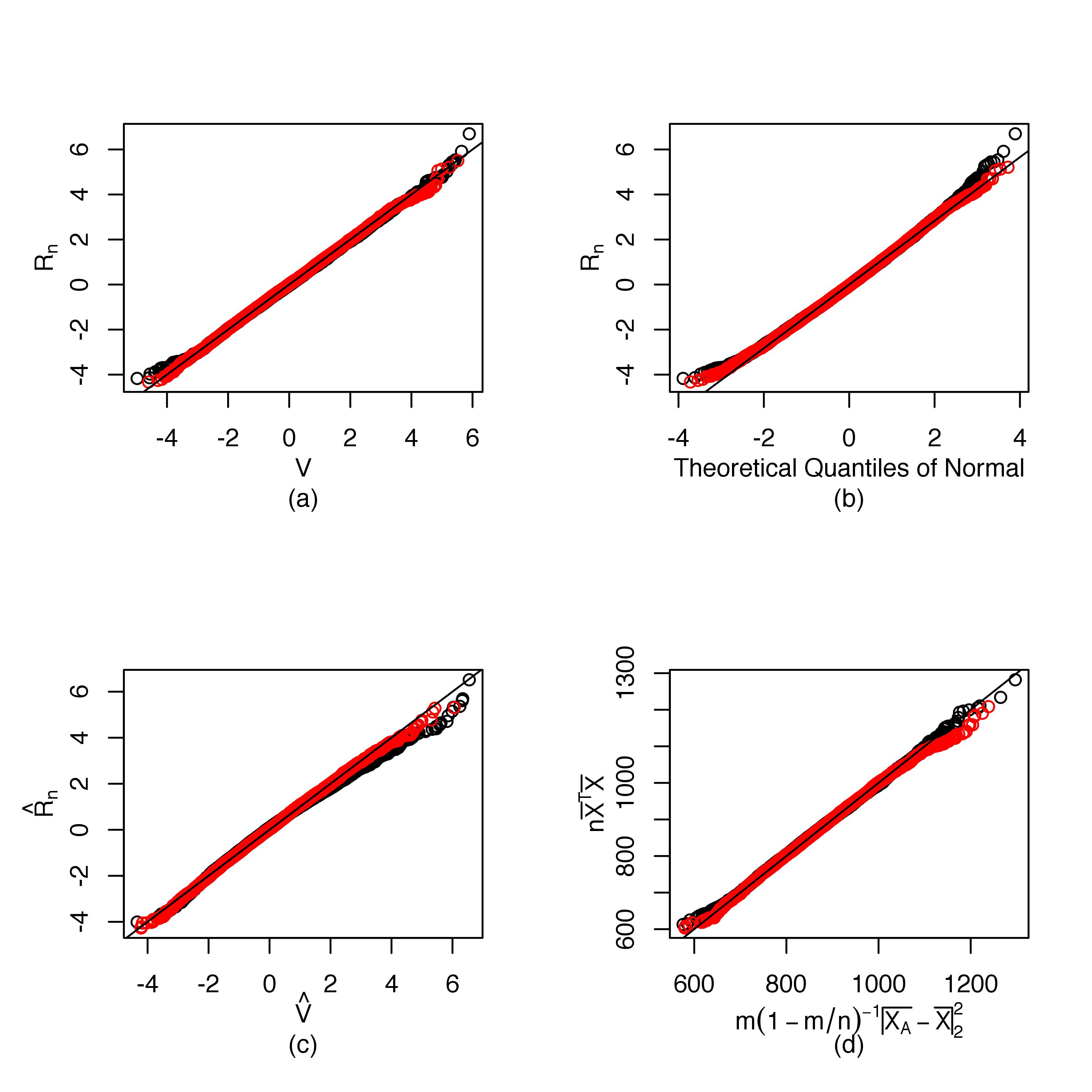
We shall use QQ plots to measure the closeness of the approximations. Recall (2.6) for VV. Figures 1(a)-4(a) show the QQ plots of the distributions of RnR_{n} and VV. In the literature majority of papers deal with central limit theorems for RnR_{n}. The normal QQ plots in Figures 1(b)-4(b) indicate that the Gaussian approximation of RnR_{n} can be quite bad if the cross-sectional dependence (among entries of X1X_{1}) is strong, see for example Model 1 with β=0.6\beta=0.6 and Model 2 with a=0.5a=0.5. In Figures 1(c)-4(c), we make QQ plots for V^\hat{V} vs R^n\hat{R}_{n}. Here V^=∑j=1pf^−1​λ^j​(ηj′−1)\hat{V}=\sum_{j=1}^{p}\hat{f}^{-1}\hat{\lambda}_{j}(\eta^{\prime}_{j}-1), where ηj′\eta^{\prime}_{j} are i.i.d. χ12\chi^{2}_{1} random variables that are independent of 𝐗n\mathbf{X}_{n} and λ^j\hat{\lambda}_{j} are eigenvalues of the sample covariance matrix Σ^=(n−1)−1​∑i=1n(Xi−X¯n)​(Xi−X¯n)T\hat{\Sigma}=(n-1)^{-1}\sum_{i=1}^{n}(X_{i}-\bar{X}_{n})(X_{i}-\bar{X}_{n})^{T}, and R^n=(n​|X¯n|22−f^1)/f†\hat{R}_{n}=(n|\bar{X}_{n}|_{2}^{2}-\hat{f}_{1})/f^{\dagger}, where f^1=tr⁡(Σ^)\hat{f}_{1}={\rm tr}(\hat{\Sigma}), and f†=[tr⁡(Σ^2)−f^12/n]1/2f^{\dagger}=[{\rm tr}(\hat{\Sigma}^{2})-\hat{f}_{1}^{2}/n]^{1/2}; see [2]. To obtain (c), the following steps are repeated for N=100N=100 times: in each realization, data is generated according to the above models. Then given Σ^\hat{\Sigma}, we obtain K=100K=100 realizations of V^\hat{V} by generating 100​p100p i.i.d. χ12\chi^{2}_{1} r.v. ηj′\eta_{j}^{\prime}. Figures 1(c)-4(c) suggest that, for the plug-in procedure, larger nn leads to better approximations. Figures 1(d)-4(d) show the subsampling procedure (cf. Theorem 3.5(ii)). As in (c), we perform in (d) the QQ plots of N=100N=100 repetitions of n​|X¯n|22n|\bar{X}_{n}|_{2}^{2} and the subsample values m​(1−m/n)−1​|X¯Aj−X¯|22m(1-m/n)^{-1}|\bar{X}_{A_{j}}-\bar{X}|_{2}^{2} with J=100J=100 and m=⌊n/log⁡n⌋m=\lfloor n/\log n\rfloor. The subsampling distribution provides an excellent approximation of the distribution of n​|X¯n|22n|\bar{X}_{n}|_{2}^{2}. For the subsampling approach one needs to choose an mm. In our simulation study for other models (not reported here) with bounded KδK_{\delta} and DδD_{\delta}, the rule-of-thumb choice m=⌊n/log⁡n⌋m=\lfloor n/\log n\rfloor can often have a satisfactory performance. We leave it as a future problem on designing a data-driven choice of mm.

Refer to caption
Figure 1: Model 1 with β=2\beta=2. (a) QQ-plot of VV v.s. RnR_{n} (cf. Theorem 2.2); (b) QQ-normal plot of RnR_{n}; (c) QQ-plot of V^\hat{V} v.s. R^n\hat{R}_{n}; (d) QQ-plot of the subsampling distribution v.s. n​|X¯|22n|\bar{X}|_{2}^{2} (cf. Theorem 3.5(ii)). Red: n=200n=200; black: n=50n=50.
Refer to caption
Figure 2: Model 1 with β=0.6\beta=0.6. See Figure 1 for the caption.
Refer to caption
Figure 3: Model 2 with a=0.05a=0.05. See Figure 1 for the caption.
Refer to caption
Figure 4: Model 2 with a=0.5a=0.5. See Figure 1 for the caption.

7 Proof

Proof of Proposition 2.1.

Note that 𝝃=Λ−1/2QTY1∼N(0,Idp){\boldsymbol{\xi}}=\Lambda^{-1/2}Q^{T}Y_{1}\sim N(0,{\rm Id}_{p}). Then Y1T​Y1=∑j=1pλj​ξj2Y_{1}^{T}Y_{1}=\sum_{j=1}^{p}\lambda_{j}\xi_{j}^{2}, where ξj\xi_{j} are entries of 𝝃{\boldsymbol{\xi}} and are i.i.d. N⁡(0,1)N(0,1). Let q=2+δq=2+\delta. By Burkholder’s inequality (Chow and Teicher [15]),

‖YT​Y−f1‖q2≤(q−1)​∑j=1pλj2​‖ξj2−1‖q2.\displaystyle\left\|Y^{T}Y-f_{1}\right\|_{q}^{2}\leq(q-1)\sum_{j=1}^{p}\lambda_{j}^{2}\|\xi^{2}_{j}-1\|_{q}^{2}.

Then (2.3) holds. Let 𝜻=Λ−1/2QTY2{\boldsymbol{\zeta}}=\Lambda^{-1/2}Q^{T}Y_{2}. Then Y1T​Y2=∑j=1pλj​ξj​ζjY_{1}^{T}Y_{2}=\sum_{j=1}^{p}\lambda_{j}\xi_{j}\zeta_{j} and (2.4) similarly follows. ∎

In Lemma 7.1 and in the proof of Theorem 2.2, we define

g0​(u)=(1−min⁡(1,max⁡(u,0))4)4.\displaystyle g_{0}(u)=(1-\min(1,\max(u,0))^{4})^{4}. (7.1)

Any non-increasing function g0​(⋅)g_{0}(\cdot) with g0​(⋅)∈ℂ3g_{0}(\cdot)\in\mathbb{C}^{3}, g0​(u)=1g_{0}(u)=1 if u≤0u\leq 0, and g0​(u)=0g_{0}(u)=0 if u≥1u\geq 1, will meet our requirements. To make the calculations explicit, we can choose g0g_{0} in the form of (7.1). Then

g∗=maxu⁡[|g0′​(u)|+|g0′′​(u)|+|g0′′′​(u)|]<∞.\displaystyle g_{*}=\max_{u}[|g^{\prime}_{0}(u)|+|g^{\prime\prime}_{0}(u)|+|g^{\prime\prime\prime}_{0}(u)|]<\infty. (7.2)
Proof of Theorem 2.2.

Let Yi∈ℝpY_{i}\in\mathbb{R}^{p} be i.i.d. N⁡(𝟎,Σ)N(\mathbf{0},\Sigma) random vectors and Y¯=∑i=1nYi/n\bar{Y}=\sum_{i=1}^{n}Y_{i}/n. Then ∑j=1pλj​ηi\sum_{j=1}^{p}{\lambda_{j}}\eta_{i} and n​|Y¯n|22n|\bar{Y}_{n}|_{2}^{2} are identically distributed. Note that f1=∑j=1pλjf_{1}=\sum_{j=1}^{p}{\lambda_{j}}. Hence, to show (2.6), since Lδ​(n,ψ)L_{\delta}(n,\psi) is increasing in ψ\psi, it suffices to prove the following relation holds for every ψ\psi:

supt|ℙ(Rn≤t)−ℙ(Rn⋄≤t)|=O(Lδ(n,ψ)+ψ−1/2),\displaystyle\sup_{t}\left|\mathbb{P}\left(R_{n}\leq t\right)-\mathbb{P}\left(R^{\diamond}_{n}\leq t\right)\right|=O(L_{\delta}(n,\psi)+\psi^{-1/2}), (7.3)

where Rn⋄R^{\diamond}_{n} is the Gaussian version of RnR_{n} in (2.5):

Rn⋄=n​|Y¯n|22−f1f.\displaystyle R^{\diamond}_{n}={{n|\bar{Y}_{n}|_{2}^{2}-f_{1}}\over f}. (7.4)

Recall (7.1) for g0g_{0}. We first approximate the indicator function h(x)=𝕀{x≤t}h(x)=\mathbb{I}\left\{x\leq t\right\} the ℂ3\mathbb{C}^{3} function gψ,t​(x)=g0​(ψ⁡(x−t))g_{\psi,t}(x)=g_{0}(\psi(x-t)) for tt fixed. By (7.2),

𝕀{x≤t}≤gψ,t(x)≤𝕀{x≤t+ψ−1},\displaystyle\mathbb{I}\left\{x\leq t\right\}\leq g_{\psi,t}(x)\leq\mathbb{I}\left\{x\leq t+\psi^{-1}\right\},
supx,t|gψ,t′​(x)|\displaystyle\quad\sup_{x,t}|g_{\psi,t}^{\prime}(x)| ≤g∗​ψ,supx,t|gψ,t′′​(x)|≤g∗​ψ2,supx,t|gψ,t′′′​(x)|≤g∗​ψ3.\displaystyle\leq g_{*}\psi,\,\,\sup_{x,t}|g_{\psi,t}^{\prime\prime}(x)|\leq g_{*}\psi^{2},\,\,\sup_{x,t}|g_{\psi,t}^{\prime\prime\prime}(x)|\leq g_{*}\psi^{3}.

Then ℙ⁡(Rn≤t)≤𝔼​gψ,t​(Rn)\mathbb{P}\left(R_{n}\leq t\right)\leq\mathbb{E}g_{\psi,t}\left(R_{n}\right). By Lemma 7.1,

𝔼​gψ,t​(Rn)\displaystyle\mathbb{E}g_{\psi,t}\left(R_{n}\right) ≤\displaystyle\leq 𝔼​gψ,t​(Rn⋄)+C​Lδ​(n,ψ)\displaystyle\mathbb{E}g_{\psi,t}\left(R^{\diamond}_{n}\right)+CL_{\delta}(n,\psi) (7.5)
≤\displaystyle\leq ℙ⁡(Rn⋄≤t+ψ−1)+C​Lδ​(n,ψ).\displaystyle\mathbb{P}\left(R^{\diamond}_{n}\leq t+\psi^{-1}\right)+CL_{\delta}(n,\psi).

The reverse direction is similar: by applying Lemma 7.1 again, we have

ℙ⁡(Rn≤t)≥ℙ⁡(Rn⋄≤t−ψ−1)−C​Lδ​(n,ψ).\displaystyle\mathbb{P}\left(R_{n}\leq t\right)\geq\mathbb{P}\left(R^{\diamond}_{n}\leq t-\psi^{-1}\right)-CL_{\delta}(n,\psi). (7.6)

By (7.5), (7.6) and (7.13) in Lemma 7.2, we have (7.3). ∎

Lemma 7.1.

Assume (2.1) and (2.2). Let K~δ\tilde{K}_{\delta} and D~δ\tilde{D}_{\delta} be specified as in Theorem 2.2. Let gψ,t​(x)=g0​(ψ⁡(x−t))g_{\psi,t}(x)=g_{0}(\psi(x-t)), where g0​(⋅)g_{0}(\cdot) is given by (7.1). Recall (7.4) for RnR_{n} and Rn⋄R^{\diamond}_{n}. Then we have

supt|𝔼​gψ,t​(Rn)−𝔼​gψ,t​(Rn⋄)|=O⁡[Lδ​(n,ψ)].\displaystyle\sup_{t}\left|\mathbb{E}g_{\psi,t}\left(R_{n}\right)-\mathbb{E}g_{\psi,t}\left(R^{\diamond}_{n}\right)\right|=O[L_{\delta}(n,\psi)]. (7.7)
Proof of Lemma 7.1.

Let Hi=∑j=1i−1Xj+∑j=i+1nYjH_{i}=\sum_{j=1}^{i-1}X_{j}+\sum_{j=i+1}^{n}Y_{j} and

Li=HiT​Hi−(n−1)​f1n​f,\displaystyle L_{i}=\frac{H_{i}^{T}H_{i}-(n-1)f_{1}}{nf},
Δi=2​HiT​Xi+XiT​Xi−f1n​f,\displaystyle\Delta_{i}=\frac{2H_{i}^{T}X_{i}+X_{i}^{T}X_{i}-f_{1}}{nf},
Γi=2​HiT​Yi+YiT​Yi−f1n​f.\displaystyle\Gamma_{i}=\frac{2H_{i}^{T}Y_{i}+Y_{i}^{T}Y_{i}-f_{1}}{nf}.

Note that HiH_{i} is independent of XiX_{i} and YiY_{i}. Let

I\displaystyle\mathrm{I} =gψ,t′​(Li)​(Δi−Γi),\displaystyle=g_{\psi,t}^{\prime}(L_{i})(\Delta_{i}-\Gamma_{i}),
II\displaystyle\mathrm{II} =12​gψ,t′′​(Li)​(Δi2−Γi2),\displaystyle=\frac{1}{2}g_{\psi,t}^{\prime\prime}(L_{i})(\Delta_{i}^{2}-\Gamma_{i}^{2}),
III\displaystyle\mathrm{III} =[gψ,t​(Li+Δi)−gψ,t​(Li+Γi)]−I−II.\displaystyle=\left[g_{\psi,t}\left(L_{i}+\Delta_{i}\right)-g_{\psi,t}\left(L_{i}+\Gamma_{i}\right)\right]-\mathrm{I}-\mathrm{II}.

Note that XiX_{i} and YiY_{i} both have mean 𝟎\mathbf{0} and covariance matrix Σ\Sigma. Then

𝔼​I\displaystyle\mathbb{E}\mathrm{I} =𝔼𝔼[gψ,t′(Li)(Δi−Γi)|Xi,Yi]\displaystyle=\mathbb{E}\mathbb{E}\left[g_{\psi,t}^{\prime}(L_{i})(\Delta_{i}-\Gamma_{i})\big|X_{i},Y_{i}\right]
=1n​f​𝔼​[2​(XiT−YiT)​𝔼​(gψ,t′​(Li)​Hi)+(XiT​Xi−YiT​Yi)​𝔼​gψ,t′​(Li)]=0.\displaystyle=\frac{1}{nf}\mathbb{E}\left[2(X_{i}^{T}-Y_{i}^{T})\mathbb{E}(g_{\psi,t}^{\prime}(L_{i})H_{i})+(X_{i}^{T}X_{i}-Y_{i}^{T}Y_{i})\mathbb{E}g_{\psi,t}^{\prime}(L_{i})\right]=0.

For II\mathrm{II}, by (7.2), |gψ,t′′​(u)|≤g∗​ψ2|g_{\psi,t}^{\prime\prime}(u)|\leq g_{*}\psi^{2}. Then for C1=g∗/2C_{1}=g_{*}/2,

|𝔼​II|\displaystyle\left|\mathbb{E}\mathrm{II}\right| =|12​𝔼​[gψ,t′′​(Li)​(Δi2−Γi2)]|\displaystyle=\left|\frac{1}{2}\mathbb{E}[g_{\psi,t}^{\prime\prime}(L_{i})(\Delta_{i}^{2}-\Gamma_{i}^{2})]\right|
=12|𝔼[gψ,t′′(Li)𝔼(Δi2−Γi2|Hi)]|\displaystyle=\frac{1}{2}\left|\mathbb{E}\left[g_{\psi,t}^{\prime\prime}(L_{i})\mathbb{E}\left(\left.\Delta_{i}^{2}-\Gamma_{i}^{2}\right|H_{i}\right)\right]\right|
≤C1ψ2𝔼|𝔼(Δi2−Γi2|Hi)|.\displaystyle\leq C_{1}\psi^{2}\mathbb{E}\left|\mathbb{E}\left(\left.\Delta_{i}^{2}-\Gamma_{i}^{2}\right|H_{i}\right)\right|.

The term n2f2𝔼(Δi2−Γi2|Hi)n^{2}f^{2}\mathbb{E}\left(\left.\Delta_{i}^{2}-\Gamma_{i}^{2}\right|H_{i}\right) can be decomposed into

4𝔼[HiTXiXiTHi−HiTYiYiTHi|Hi]+𝔼[(XiTXi−f1)2−(YiTYi−f1)2]\displaystyle 4\mathbb{E}\left[\left.H_{i}^{T}X_{i}X_{i}^{T}H_{i}-H_{i}^{T}Y_{i}Y_{i}^{T}H_{i}\right|H_{i}\right]+\mathbb{E}\left[(X_{i}^{T}X_{i}-f_{1})^{2}-(Y_{i}^{T}Y_{i}-f_{1})^{2}\right]
+4𝔼[HiTXi(XiTXi−f1)−HiTYi(YiTYi−f1)|Hi],\displaystyle\qquad+4\mathbb{E}\left[\left.H_{i}^{T}X_{i}(X_{i}^{T}X_{i}-f_{1})-H_{i}^{T}Y_{i}(Y_{i}^{T}Y_{i}-f_{1})\right|H_{i}\right],

where 𝔼(HiTXiXiTHi−HiTYiYiTHi|Hi)=0\mathbb{E}\left(\left.H_{i}^{T}X_{i}X_{i}^{T}H_{i}-H_{i}^{T}Y_{i}Y_{i}^{T}H_{i}\right|H_{i}\right)=0. By (2.1),

𝔼​|(XiT​Xi−f1)2−(YiT​Yi−f1)2|≤f2​(K02+c02)≤f2​K~02.\displaystyle\mathbb{E}\left|(X_{i}^{T}X_{i}-f_{1})^{2}-(Y_{i}^{T}Y_{i}-f_{1})^{2}\right|\leq f^{2}(K_{0}^{2}+c_{0}^{2})\leq f^{2}\tilde{K}_{0}^{2}.

Since YiY_{i} is Gaussian, 𝔼[HiTYi(YiTYi−f1)|Hi]=0\mathbb{E}\left[\left.H_{i}^{T}Y_{i}(Y_{i}^{T}Y_{i}-f_{1})\right|H_{i}\right]=0. By the Cauchy-Schwarz inequality and (2.1), since ‖HiT​Xi‖2=(n−1)​tr​(Σ2)=(n−1)​f2\|H_{i}^{T}X_{i}\|^{2}=(n-1)\mathrm{tr}(\Sigma^{2})=(n-1)f^{2},

𝔼|𝔼(Δi2−Γi2|Hi)|\displaystyle\mathbb{E}\left|\mathbb{E}\left(\left.\Delta_{i}^{2}-\Gamma_{i}^{2}\right|H_{i}\right)\right| ≤\displaystyle\leq K~02n2+𝔼|𝔼[HiTXi(XiTXi−f1)|Hi]|n2​f2\displaystyle{{\tilde{K}_{0}^{2}}\over n^{2}}+{{\mathbb{E}|\mathbb{E}[\left.H_{i}^{T}X_{i}(X_{i}^{T}X_{i}-f_{1})\right|H_{i}]|}\over{n^{2}f^{2}}}
≤\displaystyle\leq K~02n2+‖HiT​Xi‖​‖XiT​Xi−f1‖n2​f2\displaystyle{{\tilde{K}_{0}^{2}}\over n^{2}}+{{\|H_{i}^{T}X_{i}\|\|X_{i}^{T}X_{i}-f_{1}\|}\over{n^{2}f^{2}}}
≤\displaystyle\leq K~02n2+K0n3/2.\displaystyle{{\tilde{K}_{0}^{2}}\over n^{2}}+{{K_{0}}\over{n^{3/2}}}.

So

|𝔼II|≤Cψ2(n−2K~02+n−3/2K~0).\displaystyle\left|\mathbb{E}\mathrm{II}\right|\leq C\psi^{2}(n^{-2}\tilde{K}_{0}^{2}+n^{-3/2}\tilde{K}_{0}). (7.8)

Since 0≤g⁡(t)≤10\leq g(t)\leq 1 for all tt, and |gψ,t′′′​(u)|≤g∗​ψ3|g_{\psi,t}^{\prime\prime\prime}(u)|\leq g_{*}\psi^{3}. We have that

𝔼​|III|\displaystyle\mathbb{E}\left|\mathrm{III}\right| ≤𝔼​min⁡{1+|I|+|II|,g∗​ψ3​(|Δi|3+|Γi|3)}\displaystyle\leq\mathbb{E}\min\left\{1+|\mathrm{I}|+|\mathrm{II}|,g_{*}\psi^{3}(|\Delta_{i}|^{3}+|\Gamma_{i}|^{3})\right\}
≤C​𝔼​min⁡{1+ψ⁡(|Δi|+|Γi|)+ψ2​(|Δi|2+|Γi|2),ψ3​(|Δi|3+|Γi|3)}\displaystyle\leq C\mathbb{E}\min\left\{1+\psi(|\Delta_{i}|+|\Gamma_{i}|)+\psi^{2}(|\Delta_{i}|^{2}+|\Gamma_{i}|^{2}),\psi^{3}(|\Delta_{i}|^{3}+|\Gamma_{i}|^{3})\right\}
≤C​ψq​(𝔼​|Δi|q+𝔼​|Γi|q),\displaystyle\leq C\psi^{q}(\mathbb{E}\left|\Delta_{i}\right|^{q}+\mathbb{E}\left|\Gamma_{i}\right|^{q}),

where q=2+δq=2+\delta. Let 𝐱∈ℝp\mathbf{x}\in{\mathbb{R}^{p}} be a fixed vector. By Rosenthal’s inequality,

𝔼​|Hi​𝐱|qq≤cq​[m​‖X1T​𝐱‖qq+(n−m)​‖YnT​𝐱‖qq+nq/2​(𝐱T​Σ​𝐱)q/2],\displaystyle\mathbb{E}\left|H_{i}\mathbf{x}\right|_{q}^{q}\leq c_{q}[m\|X_{1}^{T}\mathbf{x}\|_{q}^{q}+(n-m)\|Y_{n}^{T}\mathbf{x}\|_{q}^{q}+n^{q/2}(\mathbf{x}^{T}\Sigma\mathbf{x})^{q/2}], (7.9)

where cqc_{q} and cq,1,…c_{q,1},\ldots hereafter are constants only depend on qq and they may take different values at different appearances. Note that YnT​𝐱∼N⁡(0,𝐱T​Σ​𝐱)Y_{n}^{T}\mathbf{x}\sim N(0,\mathbf{x}^{T}\Sigma\mathbf{x}). Let cq,1=‖ξ1‖qqc_{q,1}=\|\xi_{1}\|^{q}_{q}, ξ1∼N⁡(0,1)\xi_{1}\sim N(0,1). Then 𝔼​|YnT​𝐱|q=cq,1​(𝐱T​Σ​𝐱)q/2\mathbb{E}|Y_{n}^{T}\mathbf{x}|^{q}=c_{q,1}(\mathbf{x}^{T}\Sigma\mathbf{x})^{q/2} and

‖HiT​Xi‖qq≤cq​(n​‖X1T​X2‖qq+nq/2​𝔼​(X1T​Σ​X1)q/2)\displaystyle\|H_{i}^{T}X_{i}\|_{q}^{q}\leq c_{q}(n\left\|X_{1}^{T}X_{2}\right\|_{q}^{q}+n^{q/2}\mathbb{E}(X_{1}^{T}\Sigma X_{1})^{q/2}) (7.10)

Hence by (2.2) and (2.4), we have

𝔼​|Δi|q\displaystyle\mathbb{E}|\Delta_{i}|^{q} ≤\displaystyle\leq C​𝔼​|HiT​Xi|q+𝔼​|XiT​Xi−f1|qnq​fq\displaystyle C{{\mathbb{E}|H_{i}^{T}X_{i}|^{q}+\mathbb{E}|X_{i}^{T}X_{i}-f_{1}|^{q}}\over{n^{q}f^{q}}} (7.11)
≤\displaystyle\leq C​n​D~δq​fq+nq/2​𝔼​(X1T​Σ​X1)q/2+Kδq​fqnq​fq.\displaystyle C{{n\tilde{D}_{\delta}^{q}f^{q}+n^{q/2}\mathbb{E}(X_{1}^{T}\Sigma X_{1})^{q/2}+K_{\delta}^{q}f^{q}}\over{n^{q}f^{q}}}. (7.12)

By (7.9), ‖HiT​Yi‖qq≤cq​(n​𝔼​(X1T​Σ​X1)q/2+nq/2​fq)\|H_{i}^{T}Y_{i}\|_{q}^{q}\leq c_{q}(n\mathbb{E}(X_{1}^{T}\Sigma X_{1})^{q/2}+n^{q/2}f^{q}), which implies that 𝔼|Γi|q≤cq(n𝔼(X1TΣX1)q/2/(nf)q+n−q/2)\mathbb{E}\left|\Gamma_{i}\right|^{q}\leq c_{q}(n\mathbb{E}(X_{1}^{T}\Sigma X_{1})^{q/2}/(nf)^{q}+n^{-q/2}). Observe that (|Hi+Xi|22−n​f1)/(n​f)=Li+Δi(|H_{i}+X_{i}|_{2}^{2}-nf_{1})/(nf)=L_{i}+\Delta_{i} and (|Hi+Yi|22−n​f1)/(n​f)=Li+Γi(|H_{i}+Y_{i}|_{2}^{2}-nf_{1})/(nf)=L_{i}+\Gamma_{i}. We write the telescope sum

gψ,t​(Rn)−gψ,t​(Rn⋄)=∑i=1n[gψ,t​(Li+Δi)−gψ,t​(Li+Γi)],\displaystyle g_{\psi,t}\left(R_{n}\right)-g_{\psi,t}\left(R^{\diamond}_{n}\right)=\sum_{i=1}^{n}\left[g_{\psi,t}(L_{i}+\Delta_{i})-g_{\psi,t}(L_{i}+\Gamma_{i})\right],

which entails (7.7) in view of (7.8), (7.11) and 𝔼​I=0\mathbb{E}\mathrm{I}=0. ∎

Lemma 7.2.

Let a1≥…≥ap≥0a_{1}\geq\ldots\geq a_{p}\geq 0 be such that ∑i=1pai2=1\sum_{i=1}^{p}a_{i}^{2}=1; let ηi\eta_{i} be i.i.d. χ12\chi^{2}_{1} random variables. Then for all h>0h>0,

suptℙ⁡(t≤a1​η1+…+ap​ηp≤t+h)≤h1/2​4/π.\displaystyle\sup_{t}\mathbb{P}\left(t\leq a_{1}\eta_{1}+\ldots+a_{p}\eta_{p}\leq t+h\right)\leq h^{1/2}\sqrt{4/\pi}. (7.13)
Proof of Lemma 7.2.

Write V=∑i=1pai​ηiV=\sum_{i=1}^{p}a_{i}\eta_{i}. Assume a1≤1/2a_{1}\leq 1/2. Then its characteristic function ϕV​(s)=𝔼​exp⁡(−1​s​V),s∈ℝ\phi_{V}(s)=\mathbb{E}\exp(\sqrt{-1}sV),s\in\mathbb{R}, satisfies

|ϕV​(s)|\displaystyle|\phi_{V}(s)| =\displaystyle= |∏j=1p(1−2−1ajs)−1/2|\displaystyle\left|\prod_{j=1}^{p}(1-2\sqrt{-1}a_{j}s)^{-1/2}\right| (7.14)
=\displaystyle= ∏j=1p(1+4aj2s2)−1/4\displaystyle\prod_{j=1}^{p}(1+4a_{j}^{2}s^{2})^{-1/4} (7.15)
≤\displaystyle\leq (1+4s2+8b4s4+32/3b6s6)−1/4,\displaystyle(1+4s^{2}+8b_{4}s^{4}+32/3b_{6}s^{6})^{-1/4}, (7.16)

where b4=∑j≠kaj2​ak2=1−∑k=1pak4≥1−a12≥3/4b_{4}=\sum_{j\neq k}a_{j}^{2}a_{k}^{2}=1-\sum_{k=1}^{p}a_{k}^{4}\geq 1-a_{1}^{2}\geq 3/4 and

b6\displaystyle b_{6} =\displaystyle= ∑⋆j,k,laj2​ak2​al2=1−3​∑j≠kaj4​ak2−∑j=1paj6\displaystyle{\sum^{\star}}_{j,k,l}a_{j}^{2}a_{k}^{2}a_{l}^{2}=1-3\sum_{j\neq k}a_{j}^{4}a_{k}^{2}-\sum_{j=1}^{p}a_{j}^{6}
≥\displaystyle\geq 1−3​∑j=1paj4​(∑k≠jak2+aj2)≥1−3​a12≥1/4.\displaystyle 1-3\sum_{j=1}^{p}a_{j}^{4}\left(\sum_{k\neq j}a_{k}^{2}+a_{j}^{2}\right)\geq 1-3a_{1}^{2}\geq 1/4.

By the inversion formula and (7.14), the density function fV​(⋅)f_{V}(\cdot) of VV satisfies

fV​(v)=12​π​∫−∞∞e−−1​v​s​ϕV​(s)​𝑑s≤12​π​∫−∞∞|ϕV​(s)|​𝑑s<1\displaystyle f_{V}(v)={1\over{2\pi}}\int_{-\infty}^{\infty}e^{-\sqrt{-1}vs}\phi_{V}(s)ds\leq{1\over{2\pi}}\int_{-\infty}^{\infty}|\phi_{V}(s)|ds<1

Now we shall deal with the case that a1>1/2a_{1}>1/2. Note that for all w>0w>0, supuℙ⁡(u≤η1≤u+w)≤w1/2​2/π\sup_{u}\mathbb{P}(u\leq\eta_{1}\leq u+w)\leq w^{1/2}\sqrt{2/\pi}. Then suptℙ⁡(t≤V≤t+h)≤(2​h)1/2​2/π\sup_{t}\mathbb{P}\left(t\leq V\leq t+h\right)\leq(2h)^{1/2}\sqrt{2/\pi}. Combining with the case a1≤1/2a_{1}\leq 1/2, we obtain the upper bound max⁡(h1/2​4/π,h)\max(h^{1/2}\sqrt{4/\pi},\,h). Note that (7.13) trivially holds if h≥1h\geq 1. ∎

Proof of Proposition 3.2.

Note that ρ⁡(Σ/f)≤|Σ/f|F=1\rho(\Sigma/f)\leq|\Sigma/f|_{F}=1. Since f~/f−1=oℙ​(1)\tilde{f}/f-1=o_{\mathbb{P}}(1), ρ⁡(Σ/f)​(f/f~−1)=oℙ​(1)\rho(\Sigma/f)(f/\tilde{f}-1)=o_{\mathbb{P}}(1). Hence for the ”if” part,

ρ⁡(Σ~/f~−Σ/f)≤ρ⁡(Σ~−Σ)/f~+ρ⁡(Σ/f)​|f/f~−1|=oℙ​(1)\displaystyle\rho({\tilde{\Sigma}/\tilde{f}-\Sigma/f})\leq\rho({\tilde{\Sigma}-\Sigma})/\tilde{f}+\rho(\Sigma/f)|f/\tilde{f}-1|=o_{\mathbb{P}}(1)

The ”only if” part can be similarly proved. ∎

Proof of Lemma 3.1.

Let ρp=maxj⁡|ap,j−bp,j|\rho_{p}=\max_{j}\left|a_{p,j}-b_{p,j}\right|. Choose an integer sequence K=KpK=K_{p} such that Kp→∞K_{p}\to\infty and Kp​ρp→0K_{p}\rho_{p}\to 0. Let W=∑j=1K−1ap,j​ηj′W=\sum_{j=1}^{K-1}a_{p,j}\eta^{\prime}_{j}, W∘=∑j=Kpap,j​ηj′W^{\circ}=\sum_{j=K}^{p}a_{p,j}\eta^{\prime}_{j}, S=∑j=1K−1bp,j​ηj′S=\sum_{j=1}^{K-1}b_{p,j}\eta^{\prime}_{j}, S∘=∑j=Kpbp,j​ηj′S^{\circ}=\sum_{j=K}^{p}b_{p,j}\eta^{\prime}_{j}, w=2​∑j=Kpap,j2w=2\sum_{j=K}^{p}a_{p,j}^{2} and s=2​∑j=Kpbp,j2s=2\sum_{j=K}^{p}b_{p,j}^{2}. Let uK=ap,K1/4u_{K}=a_{p,K}^{1/4}. By the Gaussian approximation result in [39], on a richer probability space, we can construct a random variable Z∼N⁡(0,1)Z\sim N(0,1), independent of (ηi)i=1K−1(\eta_{i})_{i=1}^{K-1}, such that

ℙ⁡(|W∘−w1/2​Z|≥uK)≤c4uK4​∑j=Kpap,j4≤c4uK4​ap,K2=c4​uK4,\displaystyle\mathbb{P}(|W^{\circ}-w^{1/2}Z|\geq u_{K})\leq{c_{4}\over u_{K}^{4}}\sum_{j=K}^{p}a_{p,j}^{4}\leq{c_{4}\over u_{K}^{4}}a_{p,K}^{2}=c_{4}u_{K}^{4}, (7.17)

where c4>0c_{4}>0 is an absolute constant. Since uK→0u_{K}\to 0, by Lemma 7.2,

supx|ℙ⁡(|W+W∘|≤x)−ℙ⁡(|W+w1/2​Z|≤x)|→0.\displaystyle\sup_{x}|\mathbb{P}(|W+W^{\circ}|\leq x)-\mathbb{P}(|W+w^{1/2}Z|\leq x)|\to 0. (7.18)

Similarly, for vK=bp,K1/4v_{K}=b_{p,K}^{1/4}, we can also construct a probability space with a r.v. Z∗∼N⁡(0,1)Z^{*}\sim N(0,1) such that ℙ⁡(|S∘−w1/2​Z∗|≥vK)≤c4​vK4\mathbb{P}(|S^{\circ}-w^{1/2}Z^{*}|\geq v_{K})\leq c_{4}v_{K}^{4}, and

supx|ℙ⁡(|S+S∘|≤x)−ℙ⁡(|S+s1/2​Z∗|≤x)|→0.\displaystyle\sup_{x}|\mathbb{P}(|S+S^{\circ}|\leq x)-\mathbb{P}(|S+s^{1/2}Z^{*}|\leq x)|\to 0. (7.19)

Let T=(W+w1/2​Z)−(S+s1/2​Z)T=(W+w^{1/2}Z)-(S+s^{1/2}Z). Since w−s=2​∑j=1K−1(bp,j2−ap,j2)w-s=2\sum_{j=1}^{K-1}(b_{p,j}^{2}-a_{p,j}^{2}),

𝔼​|T|\displaystyle\mathbb{E}|T| ≤\displaystyle\leq 2​(K−1)​ρp+|w1/2−s1/2|\displaystyle 2(K-1)\rho_{p}+|w^{1/2}-s^{1/2}| (7.20)
≤\displaystyle\leq 2​K​ρp+|w−s|1/2≤2​K​ρp+(4​K​ρp)1/2→0.\displaystyle 2K\rho_{p}+|w-s|^{1/2}\leq 2K\rho_{p}+(4K\rho_{p})^{1/2}\to 0. (7.21)

Hence, by (7.18), (7.19) and Lemma 7.2, (3.4) follows. ∎

Proof of Theorem 3.3.

(i) Since XiX_{i} are i.i.d., we have

𝔼​|Σ^−Σ|F2\displaystyle\mathbb{E}|\hat{\Sigma}-\Sigma|_{F}^{2} =𝔼​∑j,k=1p(σ^j​k−σj​k)2\displaystyle=\mathbb{E}\sum_{j,k=1}^{p}(\hat{\sigma}_{jk}-\sigma_{jk})^{2}
=1n​∑j,k=1p𝔼⁡(X1​j2​X1​k2−σj​k2)\displaystyle={1\over n}\sum_{j,k=1}^{p}\mathbb{E}\left(X_{1j}^{2}X_{1k}^{2}-\sigma_{jk}^{2}\right)
=1n​𝔼​[(∑j=1pX1​j2)2]−1n​f2\displaystyle={1\over n}\mathbb{E}\Big[{\big({\sum_{j=1}^{p}X_{1j}^{2}}\big)^{2}}\Big]-{1\over n}f^{2}
=1n​𝔼​[(X1T​X1)2]−1n​f2,\displaystyle={1\over n}\mathbb{E}[(X_{1}^{T}X_{1})^{2}]-{1\over n}f^{2},

which, by the assumption 𝔼⁡[(X1T​X1)2]=o⁡(n​f2)\mathbb{E}[(X_{1}^{T}X_{1})^{2}]=o\left(nf^{2}\right), implies 𝔼​|Σ^−Σ|F2=o⁡(f2)\mathbb{E}|\hat{\Sigma}-\Sigma|_{F}^{2}=o(f^{2}). Then ‖|Σ|F−|​Σ^|F‖2≤‖|Σ^−Σ|F‖2=o⁡(f)\||\Sigma|_{F}-|\hat{\Sigma}|_{F}\|_{2}\leq\||\hat{\Sigma}-\Sigma|_{F}\|_{2}=o(f), or ‖f−f^‖2=o⁡(f)\|f-\hat{f}\|_{2}=o(f), and

‖Σ^/f^−Σ/f‖F≤‖(Σ^−Σ)/f‖F+‖|Σ^/f^|F​|1−f^/f|‖=o⁡(1).\displaystyle\|\hat{\Sigma}/\hat{f}-\Sigma/f\|_{F}\leq\|(\hat{\Sigma}-\Sigma)/f\|_{F}+\||\hat{\Sigma}/\hat{f}|_{F}|1-\hat{f}/f|\|=o(1).

(ii) Let g=‖X1T​X1‖g=\|X_{1}^{T}X_{1}\|. Since n​f2=o⁡(g2)nf^{2}=o(g^{2}), by Schwarz’s inequality,

𝔼⁡[(X1T​Σ​X1)2]\displaystyle\mathbb{E}[(X_{1}^{T}\Sigma X_{1})^{2}] ≤\displaystyle\leq 𝔼⁡(X1T​Σ2​X1​X1T​X1)=𝔼​tr​[(X1​X1T)2​Σ2]\displaystyle\mathbb{E}(X_{1}^{T}\Sigma^{2}X_{1}X_{1}^{T}X_{1})=\mathbb{E}\mathrm{tr}[(X_{1}X_{1}^{T})^{2}\Sigma^{2}] (7.22)
≤\displaystyle\leq 𝔼⁡[tr⁡(Σ4)​(X1T​X1)2]≤f2​g2=o⁡(g4n).\displaystyle\mathbb{E}[\sqrt{\mathrm{tr}(\Sigma^{4})}(X_{1}^{T}X_{1})^{2}]\leq f^{2}g^{2}=o({g^{4}\over n}). (7.23)

Since (2.1) holds with K2=O⁡(n3/4)K_{2}=O(n^{3/4}) and 𝔼⁡(X1T​X1)=f1≤g\mathbb{E}(X_{1}^{T}X_{1})=f_{1}\leq g, we have

‖X1T​X1‖44≤8​‖X1T​X1−f1‖44+8​f14≤8​K24​f4+8​f14=o⁡(n​g4).\displaystyle\left\|X_{1}^{T}X_{1}\right\|_{4}^{4}\leq 8\left\|X_{1}^{T}X_{1}-f_{1}\right\|_{4}^{4}+8f_{1}^{4}\leq 8K_{2}^{4}f^{4}+8f_{1}^{4}=o(ng^{4}). (7.24)

By (7.24) and (7.22), we have

𝔼⁡[(X1T​X1)2​X1T​Σ​X1]≤{𝔼⁡[(X1T​X1)4]​𝔼​[(X1T​Σ​X1)2]}1/2=o⁡(g4).\displaystyle\mathbb{E}[(X_{1}^{T}X_{1})^{2}X_{1}^{T}\Sigma X_{1}]\leq\{{\mathbb{E}[(X_{1}^{T}X_{1})^{4}]}{\mathbb{E}[(X_{1}^{T}\Sigma X_{1})^{2}]}\}^{1/2}=o(g^{4}). (7.25)

Since 𝔼⁡[(X1T​X1)2​(X1T​X2)2]=𝔼⁡[(X1T​X1)2​X1T​Σ​X1]\mathbb{E}[(X_{1}^{T}X_{1})^{2}(X_{1}^{T}X_{2})^{2}]=\mathbb{E}[(X_{1}^{T}X_{1})^{2}X_{1}^{T}\Sigma X_{1}], by (7.25), we have

𝔼⁡[X1T​X1​(X1T​X2)2​X2T​X2]≤𝔼⁡[(X1T​X1)2​(X1T​X2)2]=o⁡(g4)\displaystyle\mathbb{E}[X_{1}^{T}X_{1}(X_{1}^{T}X_{2})^{2}X_{2}^{T}X_{2}]\leq\mathbb{E}[(X_{1}^{T}X_{1})^{2}(X_{1}^{T}X_{2})^{2}]=o(g^{4}) (7.26)

Since (ρ⁡(Σ^)/f^)4≤f^44/f^4≤(ρ⁡(Σ^)/f^)2(\rho(\hat{\Sigma})/\hat{f})^{4}\leq{\hat{f}_{4}^{4}/\hat{f}^{4}}\leq(\rho(\hat{\Sigma})/\hat{f})^{2}, it suffices to show that f^44/f^4=oℙ​(1)\hat{f}_{4}^{4}/\hat{f}^{4}=o_{\mathbb{P}}(1). Clearly the latter follows from

𝔼⁡(f^44)=o⁡(𝔼2​(f^2))​ and ​𝔼​(f^2/𝔼⁡(f^2)−1)2=o⁡(1).\displaystyle\mathbb{E}(\hat{f}_{4}^{4})=o(\mathbb{E}^{2}(\hat{f}^{2}))\mbox{ and }\mathbb{E}(\hat{f}^{2}/\mathbb{E}(\hat{f}^{2})-1)^{2}=o(1). (7.27)

An expansion of f^2=∑j,k≤pσ^j​k2\hat{f}^{2}=\sum_{j,k\leq p}\hat{\sigma}_{jk}^{2} yields that

n2​𝔼​(f^2)\displaystyle n^{2}\mathbb{E}(\hat{f}^{2}) =∑1≤i≠l≤n,1≤j,k≤p𝔼⁡(Xi​j​Xi​k​Xl​j​Xl​k)+∑1≤i≤n,1≤j,k≤p𝔼⁡(Xi​j2​Xi​k2)\displaystyle={\sum_{1\leq i\neq l\leq n,1\leq j,k\leq p}\mathbb{E}(X_{ij}X_{ik}X_{lj}X_{lk})+\sum_{1\leq i\leq n,1\leq j,k\leq p}\mathbb{E}(X^{2}_{ij}X^{2}_{ik})}
=n⁡(n−1)​∑j,k=1pσj​k2+n​∑j,k=1p𝔼⁡(Xi​j2​Xi​k2)\displaystyle={n(n-1)\sum_{j,k=1}^{p}\sigma_{jk}^{2}+n\sum_{j,k=1}^{p}\mathbb{E}(X^{2}_{ij}X^{2}_{ik})}
=(n2−n)​f2+n​𝔼​[(X1T​X1)2].\displaystyle=(n^{2}-n)f^{2}+n\mathbb{E}[(X_{1}^{T}X_{1})^{2}].

Since n​f2=o⁡(g2)nf^{2}=o(g^{2}), we have 𝔼⁡(f^2)≍n−1​g2\mathbb{E}(\hat{f}^{2})\asymp n^{-1}g^{2}. Write

n4​𝔼​(tr⁡(Σ^4))\displaystyle n^{4}\mathbb{E}(\mathrm{tr}(\hat{\Sigma}^{4})) =∑1≤j,k,m,q≤p∑1≤i,l,s,t≤n𝔼⁡(Xi​j​Xi​k​Xl​k​Xl​m​Xs​m​Xs​q​Xt​q​Xt​j)\displaystyle=\sum_{1\leq j,k,m,q\leq p}\sum_{1\leq i,l,s,t\leq n}\mathbb{E}\left(X_{ij}X_{ik}X_{lk}X_{lm}X_{sm}X_{sq}X_{tq}X_{tj}\right)
=:I+II+III+IV+V+VI+VII,\displaystyle=:\mathrm{I}+\mathrm{II}+\mathrm{III}+\mathrm{IV}+\mathrm{V}+\mathrm{VI}+\mathrm{VII},

where, based on the number of distinct indexes in {i,l,s,t}\{i,l,s,t\},

I=\displaystyle\mathrm{I}= n⁡(n−1)​(n−2)​(n−3)​∑1≤j,k,m,q≤pσj​k​σk​m​σm​q​σq​j\displaystyle n(n-1)(n-2)(n-3)\sum_{1\leq j,k,m,q\leq p}\sigma_{jk}\sigma_{km}\sigma_{mq}\sigma_{qj}
II=\displaystyle\mathrm{II}= 4​n​(n−1)​(n−2)​∑1≤j,k,m,q≤p𝔼⁡(X1​j​X1​k2​X1​m)​σm​q​σq​j\displaystyle 4n(n-1)(n-2)\sum_{1\leq j,k,m,q\leq p}\mathbb{E}\left(X_{1j}X_{1k}^{2}X_{1m}\right)\sigma_{mq}\sigma_{qj}
III=\displaystyle\mathrm{III}= 2​n​(n−1)​(n−2)​∑1≤j,k,m,q≤p𝔼⁡(X1​j​X1​k​X1​m​X1​q)​σk​m​σq​j\displaystyle 2n(n-1)(n-2)\sum_{1\leq j,k,m,q\leq p}\mathbb{E}\left(X_{1j}X_{1k}X_{1m}X_{1q}\right)\sigma_{km}\sigma_{qj}
IV=\displaystyle\mathrm{IV}= 2​n​(n−1)​∑1≤j,k,m,q≤p𝔼⁡(X1​j​X1​k2​X1​m)​𝔼​(X1​m​X1​q2​X1​j)\displaystyle 2n(n-1)\sum_{1\leq j,k,m,q\leq p}\mathbb{E}\left(X_{1j}X_{1k}^{2}X_{1m}\right)\mathbb{E}\left(X_{1m}X_{1q}^{2}X_{1j}\right)
V=\displaystyle\mathrm{V}= n⁡(n−1)​∑1≤j,k,m,q≤p[𝔼⁡(X1​j​X1​k​X1​m​X1​q)]2\displaystyle n(n-1)\sum_{1\leq j,k,m,q\leq p}\left[\mathbb{E}\left(X_{1j}X_{1k}X_{1m}X_{1q}\right)\right]^{2}
VI=\displaystyle\mathrm{VI}= 4​n​(n−1)​∑1≤j,k,m,q≤pσj​k​𝔼​(X1​j​X1​k​X1​m2​X1​q2)\displaystyle 4n(n-1)\sum_{1\leq j,k,m,q\leq p}\sigma_{jk}\mathbb{E}\left(X_{1j}X_{1k}X_{1m}^{2}X_{1q}^{2}\right)
VII=\displaystyle\mathrm{VII}= n​∑1≤j,k,m,q≤p𝔼⁡(X1​j2​X1​k2​X1​m2​X1​q2).\displaystyle n\sum_{1\leq j,k,m,q\leq p}\mathbb{E}\left(X_{1j}^{2}X_{1k}^{2}X_{1m}^{2}X_{1q}^{2}\right).

Note that tr⁡(Σk/fk)≤ρ​(Σ/f)k−2=o⁡(1)\mathrm{tr}(\Sigma^{k}/f^{k})\leq\rho(\Sigma/f)^{k-2}=o(1) for k>2k>2. By (3.8) and (7.22)–(7.26), we obtain by elementary manipulations that 𝔼⁡(f^44)=o⁡(𝔼2​(f^2))\mathbb{E}(\hat{f}_{4}^{4})=o(\mathbb{E}^{2}(\hat{f}^{2})). To prove the second assertion of (7.27), we similarly write

n4​𝔼​f^4\displaystyle n^{4}\mathbb{E}\hat{f}^{4} =∑1≤j,k,m,q≤p∑1≤i,l,s,t≤n𝔼⁡(Xi​j​Xi​k​Xl​j​Xl​k​Xs​m​Xs​q​Xt​m​Xt​q)\displaystyle=\sum_{1\leq j,k,m,q\leq p}\sum_{1\leq i,l,s,t\leq n}\mathbb{E}\left(X_{ij}X_{ik}X_{lj}X_{lk}X_{sm}X_{sq}X_{tm}X_{tq}\right)
=I′+II′+III′+IV′+V′+VI′+VII′,\displaystyle=\mathrm{I}^{\prime}+\mathrm{II}^{\prime}+\mathrm{III}^{\prime}+\mathrm{IV}^{\prime}+\mathrm{V}^{\prime}+\mathrm{VI}^{\prime}+\mathrm{VII}^{\prime},

where

I′:=\displaystyle\mathrm{I}^{\prime}:= n⁡(n−1)​(n−2)​(n−3)​∑1≤j,k,m,q≤pσj​k2​σm​q2\displaystyle n(n-1)(n-2)(n-3)\sum_{1\leq j,k,m,q\leq p}\sigma_{jk}^{2}\sigma_{mq}^{2}
II′:=\displaystyle\mathrm{II}^{\prime}:= 2​n​(n−1)​(n−2)​∑1≤j,k,m,q≤p𝔼⁡(X1​j2​X1​k2)​σm​q2\displaystyle 2n(n-1)(n-2)\sum_{1\leq j,k,m,q\leq p}\mathbb{E}\left(X_{1j}^{2}X_{1k}^{2}\right)\sigma_{mq}^{2}
III′:=\displaystyle\mathrm{III}^{\prime}:= 4​n​(n−1)​(n−2)​∑1≤j,k,m,q≤p𝔼⁡(X1​j​X1​k​X1​m​X1​q)​σj​k​σm​q\displaystyle 4n(n-1)(n-2)\sum_{1\leq j,k,m,q\leq p}\mathbb{E}\left(X_{1j}X_{1k}X_{1m}X_{1q}\right)\sigma_{jk}\sigma_{mq}
IV′:=\displaystyle\mathrm{IV}^{\prime}:= 4​n​(n−1)​∑1≤j,k,m,q≤pσj​k​𝔼​(X1​j​X1​k​X1​m2​X1​q2)\displaystyle 4n(n-1)\sum_{1\leq j,k,m,q\leq p}\sigma_{jk}\mathbb{E}\left(X_{1j}X_{1k}X_{1m}^{2}X_{1q}^{2}\right)
V′:=\displaystyle\mathrm{V}^{\prime}:= n⁡(n−1)​∑1≤j,k,m,q≤p𝔼⁡(X1​j2​X1​k2)​𝔼​(X1​m2​X1​q2)\displaystyle n(n-1)\sum_{1\leq j,k,m,q\leq p}\mathbb{E}\left(X_{1j}^{2}X_{1k}^{2}\right)\mathbb{E}\left(X_{1m}^{2}X_{1q}^{2}\right)
VI′:=\displaystyle\mathrm{VI}^{\prime}:= 2​n​(n−1)​∑1≤j,k,m,q≤p[𝔼⁡(X1​j​X1​k​X1​m​X1​q)]2\displaystyle 2n(n-1)\sum_{1\leq j,k,m,q\leq p}\left[\mathbb{E}\left(X_{1j}X_{1k}X_{1m}X_{1q}\right)\right]^{2}
VII′:=\displaystyle\mathrm{VII}^{\prime}:= n​∑1≤j,k,m,q≤p𝔼⁡(X1​j2​X1​k2​X1​m2​X1​q2).\displaystyle n\sum_{1\leq j,k,m,q\leq p}\mathbb{E}\left(X_{1j}^{2}X_{1k}^{2}X_{1m}^{2}X_{1q}^{2}\right).

Then the second assertion of (7.27) similarly follows from (3.8), (7.22)–(7.26). ∎

Proof of Theorem 5.2.

Write WW and W∗W^{*} for W1W_{1} and W2W_{2}, respectively. Let B=AT​AB=A^{T}A and U=A​𝝃U=A{\boldsymbol{\xi}}. Then f1=tr⁡(B)f_{1}=\mathrm{tr}(B), UT​Σ​U=𝝃T​B2​𝝃U^{T}\Sigma U={\boldsymbol{\xi}}^{T}B^{2}{\boldsymbol{\xi}} and UT​U=𝝃T​B​𝝃U^{T}U={\boldsymbol{\xi}}^{T}B{\boldsymbol{\xi}}. By the argument in (4.8), we have ‖UT​U−f1‖q2≤4​q2​‖ξ12‖q2​f2\left\|U^{T}U-f_{1}\right\|^{2}_{q}\leq 4q^{2}\|\xi_{1}^{2}\|_{q}^{2}f^{2},

‖UT​Σ​U−f2‖q2\displaystyle\left\|U^{T}\Sigma U-f^{2}\right\|_{q}^{2} ≤\displaystyle\leq 4​q2​‖ξ12‖q2​tr​(B4)≤4​q2​‖ξ12‖q2​f4,\displaystyle 4q^{2}\|\xi_{1}^{2}\|_{q}^{2}\mathrm{tr}(B^{4})\leq 4q^{2}\|\xi_{1}^{2}\|_{q}^{2}f^{4},
‖(UT​U−f1)2‖q\displaystyle\left\|(U^{T}U-f_{1})^{2}\right\|_{q} =\displaystyle= ‖UT​U−f1‖2​q2≤4​(2​q)2​‖ξ12‖2​q2​f2\displaystyle\left\|U^{T}U-f_{1}\right\|_{2q}^{2}\leq 4(2q)^{2}\|\xi_{1}^{2}\|_{2q}^{2}f^{2}

By the identity in (5.9), note that (UT​U)2=(UT​U−f1)2+2​f1​(UT​U−f1)+f12(U^{T}U)^{2}=(U^{T}U-f_{1})^{2}+2f_{1}(U^{T}U-f_{1})+f_{1}^{2}, we obtain (5.14) with C¯δ=2​(4​q​‖ξ12‖2​q)2​q\bar{C}_{\delta}=2(4q\|\xi_{1}^{2}\|_{2q})^{2q}.

Let U∗=A​𝜻U^{*}=A{\boldsymbol{\zeta}}, where 𝜻{\boldsymbol{\zeta}} and 𝝃{\boldsymbol{\xi}} are i.i.d. Then UT​U∗=𝝃T​B​𝜻U^{T}U^{*}={\boldsymbol{\xi}}^{T}B{\boldsymbol{\zeta}}. By (4.4), ‖𝝃T​B​𝜻‖2​q2≤(2​q−1)2​‖ξ1‖2​q4​f2\left\|{\boldsymbol{\xi}}^{T}B{\boldsymbol{\zeta}}\right\|_{2q}^{2}\leq(2q-1)^{2}\left\|\xi_{1}\right\|_{2q}^{4}f^{2}, which similarly implies (5.15) with D¯δ=(4​q)q​‖ξ1‖2​q2​q+(2​q−1)2​q​‖ξ1‖2​q4​q\bar{D}_{\delta}=(4q)^{q}\left\|\xi_{1}\right\|_{2q}^{2q}+(2q-1)^{2q}\left\|\xi_{1}\right\|_{2q}^{4q} in view of the second identity in (5.9). ∎

Proof of Lemma 5.1.

Let ℬ=((i,j),1≤i≤j≤p)\mathcal{B}=\left((i,j),1\leq i\leq j\leq p\right) and 𝝎=(ωb)b∈ℬ∈ℝp⁡(p+1)/2{\boldsymbol{\omega}}=\left(\omega_{b}\right)_{b\in\mathcal{B}}\in\mathbb{R}^{p(p+1)/2}, where ωb=ξiξj−𝕀{i=j}\omega_{b}=\xi_{i}\xi_{j}-\mathbb{I}\left\{i=j\right\} for b=(i,j)b=(i,j), that is

𝝎=(ϱ1,ξ1​ξ2,…,ξ1​ξp,ϱ2,ξ2​ξ3,…,ϱp)T, where ​ϱk=ξk2−1.\displaystyle{\boldsymbol{\omega}}=\left(\varrho_{1},\xi_{1}\xi_{2},\ldots,\xi_{1}\xi_{p},\varrho_{2},\xi_{2}\xi_{3},\ldots,\varrho_{p}\right)^{T},\mbox{ where }\varrho_{k}=\xi_{k}^{2}-1.

Let VWV_{W} be the covariance matrix of 𝝎{\boldsymbol{\omega}}. Then VW=diag⁡({vb,b}b∈ℬ)V_{W}=\mathrm{diag}\left(\left\{v_{b,b}\right\}_{b\in\mathcal{B}}\right), where for b=(i,l)b=\left(i,l\right), vb,b=Var⁡(ξi2)v_{b,b}=\mathrm{Var}\left(\xi_{i}^{2}\right) if l=il=i and vb,b=1v_{b,b}=1 if l≠il\not=i. Also define G=(ga,b)a∈ℐ,b∈ℬ∈ℝp2×[p⁡(p+1)/2]G=\left(g_{a,b}\right)_{a\in\mathcal{I},b\in\mathcal{B}}\in\mathbb{R}^{p^{2}\times\left[p(p+1)/2\right]}, where for a=(j,k)a=\left(j,k\right), b=(i,l)b=\left(i,l\right),

ga,b={aj​i​ak​i, if ​l=i;aj​i​ak​l+aj​l​ak​i, if ​i<l.\displaystyle g_{a,b}=\begin{cases}a_{ji}a_{ki},&\mbox{ if }l=i;\\ a_{ji}a_{kl}+a_{jl}a_{ki},&\mbox{ if }i<l.\end{cases}

Note that Xj​Xk=𝐠aT​𝝎,X_{j}X_{k}=\mathbf{g}_{a}^{T}{\boldsymbol{\omega}}, where 𝐠aT\mathbf{g}_{a}^{T} is the aa’th row of GG. Then W=G​𝝎W=G{\boldsymbol{\omega}} and

𝔼⁡(W​WT)=(γa,a′)a,a′∈ℐ,\displaystyle\mathbb{E}\left(WW^{T}\right)=\left(\gamma_{a,a^{\prime}}\right)_{a,a^{\prime}\in\mathcal{I}},

where for a=(j,k)a=(j,k), a′=(m,q)a^{\prime}=(m,q),

γa,a′\displaystyle\gamma_{a,a^{\prime}} =\displaystyle= cov⁡(Xj​Xk,Xm​Xq)=𝐠aT​VW​𝐠a′\displaystyle\mathrm{cov}\left(X_{j}X_{k},X_{m}X_{q}\right)=\mathbf{g}_{a}^{T}V_{W}\mathbf{g}_{a^{\prime}} (7.28)
=\displaystyle= ν​∑iaj​i​ak​i​am​i​aq​i+∑i<l(aj​i​ak​l+aj​l​ak​i)​(aq​i​am​l+am​i​aq​l)\displaystyle\nu\sum_{i}a_{ji}a_{ki}a_{mi}a_{qi}+\sum_{i<l}\left(a_{ji}a_{kl}+a_{jl}a_{ki}\right)\left(a_{qi}a_{ml}+a_{mi}a_{ql}\right) (7.29)
=\displaystyle= (ν−2)​∑iaj​i​ak​i​am​i​aq​i+σj​m​σk​q+σj​q​σk​m.\displaystyle(\nu-2)\sum_{i}a_{ji}a_{ki}a_{mi}a_{qi}+\sigma_{jm}\sigma_{kq}+\sigma_{jq}\sigma_{km}. (7.30)

Let B=AT​A=(bi​l)i,lB=A^{T}A=\left(b_{il}\right)_{i,l}, L0=2​f4+2​f44L_{0}=2f^{4}+2f_{4}^{4}, L1=∑i​lbi​l4L_{1}=\sum_{il}b_{il}^{4} and L2=∑i(∑lbi​l2)2L_{2}=\sum_{i}\left(\sum_{l}b_{il}^{2}\right)^{2}. By (7.28),

fW2\displaystyle f_{W}^{2} =∑a,a′∈ℐγa,a′2\displaystyle=\sum_{a,a^{\prime}\in\mathcal{I}}\gamma_{a,a^{\prime}}^{2}
=∑1≤j,k,m,q≤p[(ν−2)​∑iaj​i​ak​i​am​i​aq​i+σj​m​σk​q+σj​q​σk​m]2\displaystyle=\sum_{1\leq j,k,m,q\leq p}\big[{(\nu-2)\sum_{i}a_{ji}a_{ki}a_{mi}a_{qi}+\sigma_{jm}\sigma_{kq}+\sigma_{jq}\sigma_{km}}\big]^{2}
=L1​(ν−2)2+4​L2​(ν−2)+L0.\displaystyle=L_{1}(\nu-2)^{2}+4L_{2}(\nu-2)+L_{0}.

Clearly fW2≥2​f4f_{W}^{2}\geq 2f^{4} if ν≥2\nu\geq 2. Note that 4​L1−8​L2+L0≥04L_{1}-8L_{2}+L_{0}\geq 0. Since L1≤L2L_{1}\leq L_{2}, L0≥8​L2−4​L1≥4​L1L_{0}\geq 8L_{2}-4L_{1}\geq 4L_{1}. If 0<ν<20<\nu<2, then the quantity

fW2−L0​ν24=(L1−L04)​ν2+4​(L2−L1)​ν+L0+4​L1−8​L2f_{W}^{2}-\frac{L_{0}\nu^{2}}{4}=\left(L_{1}-\frac{L_{0}}{4}\right)\nu^{2}+4(L_{2}-L_{1})\nu+L_{0}+4L_{1}-8L_{2}

is larger than the minimum of its value at ν=0\nu=0 and ν=2\nu=2, which are both nonnegative. Therefore, fW2≥ν2​f4/2f_{W}^{2}\geq\nu^{2}f^{4}/2 for any ν∈(0,2)\nu\in(0,2). ∎

References

  • [1] T. W. Anderson. An introduction to multivariate statistical analysis. Wiley Series in Probability and Statistics. Wiley-Interscience [John Wiley & Sons], Hoboken, NJ, third edition, 2003. ISBN 0-471-36091-0.
  • [2] Zhidong Bai and Hewa Saranadasa. Effect of high dimension: by an example of a two sample problem. Statist. Sinica, 6(2):311–329, 1996. ISSN 1017-0405.
  • [3] Zhidong Bai and Jack W. Silverstein. Spectral analysis of large dimensional random matrices. Springer Series in Statistics. Springer, New York, second edition, 2010. ISBN 978-1-4419-0660-1. doi: 10.1007/978-1-4419-0661-8. URL http://dx.doi.org/10.1007/978-1-4419-0661-8.
  • [4] Zhidong Bai, Dandan Jiang, Jian-Feng Yao, and Shurong Zheng. Corrections to LRT on large-dimensional covariance matrix by RMT. Ann. Statist., 37(6B):3822–3840, 2009. ISSN 0090-5364. doi: 10.1214/09-AOS694. URL http://dx.doi.org/10.1214/09-AOS694.
  • [5] V. Bentkus. On the dependence of the Berry-Esseen bound on dimension. J. Statist. Plann. Inference, 113(2):385–402, 2003. ISSN 0378-3758. doi: 10.1016/S0378-3758(02)00094-0. URL http://dx.doi.org/10.1016/S0378-3758(02)00094-0.
  • [6] V. Bentkus. A Lyapunov type bound in 𝐑d{\bf R}^{d}. Teor. Veroyatn. Primen., 49(2):400–410, 2004. ISSN 0040-361X. doi: 10.1137/S0040585X97981123. URL http://dx.doi.org/10.1137/S0040585X97981123.
  • [7] István Berkes, Weidong Liu, and Wei Biao Wu. Komlós-Major-Tusnády approximation under dependence. Ann. Probab., 42(2):794–817, 2014. ISSN 0091-1798. doi: 10.1214/13-AOP850. URL http://dx.doi.org/10.1214/13-AOP850.
  • [8] Peter J. Bickel and Elizaveta Levina. Regularized estimation of large covariance matrices. Ann. Statist., 36(1):199–227, 2008a. ISSN 0090-5364. doi: 10.1214/009053607000000758. URL http://dx.doi.org/10.1214/009053607000000758.
  • [9] Peter J. Bickel and Elizaveta Levina. Covariance regularization by thresholding. Ann. Statist., 36(6):2577–2604, 2008b. ISSN 0090-5364. doi: 10.1214/08-AOS600. URL http://dx.doi.org/10.1214/08-AOS600.
  • [10] Melanie Birke and Holger Dette. A note on testing the covariance matrix for large dimension. Statist. Probab. Lett., 74(3):281–289, 2005. ISSN 0167-7152. doi: 10.1016/j.spl.2005.04.051. URL http://dx.doi.org/10.1016/j.spl.2005.04.051.
  • [11] T. Tony Cai and Zongming Ma. Optimal hypothesis testing for high dimensional covariance matrices. Bernoulli, 19(5B):2359–2388, 2013. ISSN 1350-7265. doi: 10.3150/12-BEJ455. URL http://dx.doi.org/10.3150/12-BEJ455.
  • [12] Song Xi Chen and Ying-Li Qin. A two-sample test for high-dimensional data with applications to gene-set testing. Ann. Statist., 38(2):808–835, 2010. ISSN 0090-5364. doi: 10.1214/09-AOS716. URL http://dx.doi.org/10.1214/09-AOS716.
  • [13] Song Xi Chen, Li-Xin Zhang, and Ping-Shou Zhong. Tests for high-dimensional covariance matrices. J. Amer. Statist. Assoc., 105(490):810–819, 2010. ISSN 0162-1459. doi: 10.1198/jasa.2010.tm09560. URL http://dx.doi.org/10.1198/jasa.2010.tm09560.
  • [14] Victor Chernozhukov, Denis Chetverikov, and Kengo Kato. Gaussian approximations and multiplier bootstrap for maxima of sums of high-dimensional random vectors. Ann. Statist., 41(6):2786–2819, 2013. ISSN 0090-5364. doi: 10.1214/13-AOS1161. URL http://dx.doi.org/10.1214/13-AOS1161.
  • [15] Yuan Shih Chow and Henry Teicher. Probability theory. Springer Texts in Statistics. Springer-Verlag, New York, third edition, 1997. ISBN 0-387-98228-0. doi: 10.1007/978-1-4612-1950-7. URL http://dx.doi.org/10.1007/978-1-4612-1950-7. Independence, interchangeability, martingales.
  • [16] A. P. Dempster. A high dimensional two sample significance test. Ann. Math. Statist., 29:995–1010, 1958. ISSN 0003-4851.
  • [17] A. P. Dempster. A significance test for the separation of two highly multivariate small samples. Biometrics, 16:41–50, 1960. ISSN 0006-341X.
  • [18] Noureddine El Karoui. Spectrum estimation for large dimensional covariance matrices using random matrix theory. Ann. Statist., 36(6):2757–2790, 2008. ISSN 0090-5364. doi: 10.1214/07-AOS581. URL http://dx.doi.org/10.1214/07-AOS581.
  • [19] Jianqing Fan, Peter Hall, and Qiwei Yao. To how many simultaneous hypothesis tests can normal, Student’s tt or bootstrap calibration be applied? J. Amer. Statist. Assoc., 102(480):1282–1288, 2007. ISSN 0162-1459. doi: 10.1198/016214507000000969. URL http://dx.doi.org/10.1198/016214507000000969.
  • [20] Thomas J. Fisher, Xiaoqian Sun, and Colin M. Gallagher. A new test for sphericity of the covariance matrix for high dimensional data. J. Multivariate Anal., 101(10):2554–2570, 2010. ISSN 0047-259X. doi: 10.1016/j.jmva.2010.07.004. URL http://dx.doi.org/10.1016/j.jmva.2010.07.004.
  • [21] Stuart Geman. A limit theorem for the norm of random matrices. Ann. Probab., 8(2):252–261, 1980. ISSN 0091-1798. URL http://links.jstor.org/sici?sici=0091-1798(198004)8:2<252:ALTFTN>2.0.CO;2-4&origin=MSN.
  • [22] Gene H. Golub and Charles F. Van Loan. Matrix computations. Johns Hopkins Studies in the Mathematical Sciences. Johns Hopkins University Press, Baltimore, MD, fourth edition, 2013. ISBN 978-1-4214-0794-4; 1-4214-0794-9; 978-1-4214-0859-0.
  • [23] Dandan Jiang, Tiefeng Jiang, and Fan Yang. Likelihood ratio tests for covariance matrices of high-dimensional normal distributions. J. Statist. Plann. Inference, 142(8):2241–2256, 2012. ISSN 0378-3758. doi: 10.1016/j.jspi.2012.02.057. URL http://dx.doi.org/10.1016/j.jspi.2012.02.057.
  • [24] S. John. The distribution of a statistic used for testing sphericity of normal distributions. Biometrika, 59:169–173, 1972. ISSN 0006-3444.
  • [25] Iain M. Johnstone. On the distribution of the largest eigenvalue in principal components analysis. Ann. Statist., 29(2):295–327, 2001. ISSN 0090-5364. doi: 10.1214/aos/1009210544. URL http://dx.doi.org/10.1214/aos/1009210544.
  • [26] Shota Katayama and Yutaka Kano. A new test on high-dimensional mean vector without any assumption on population covariance matrix.
  • [27] Shota Katayama, Yutaka Kano, and Muni S. Srivastava. Asymptotic distributions of some test criteria for the mean vector with fewer observations than the dimension. J. Multivariate Anal., 116:410–421, 2013. ISSN 0047-259X. doi: 10.1016/j.jmva.2013.01.008. URL http://dx.doi.org/10.1016/j.jmva.2013.01.008.
  • [28] Michael R. Kosorok and Shuangge Ma. Marginal asymptotics for the “large pp, small nn” paradigm: with applications to microarray data. Ann. Statist., 35(4):1456–1486, 2007. ISSN 0090-5364. doi: 10.1214/009053606000001433. URL http://dx.doi.org/10.1214/009053606000001433.
  • [29] Olivier Ledoit and Michael Wolf. Some hypothesis tests for the covariance matrix when the dimension is large compared to the sample size. Ann. Statist., 30(4):1081–1102, 2002. ISSN 0090-5364. doi: 10.1214/aos/1031689018. URL http://dx.doi.org/10.1214/aos/1031689018.
  • [30] Weidong Liu and Qi-Man Shao. A Carmér moderate deviation theorem for Hotelling’s T2T^{2}-statistic with applications to global tests. Ann. Statist., 41(1):296–322, 2013. ISSN 0090-5364. doi: 10.1214/12-AOS1082. URL http://dx.doi.org/10.1214/12-AOS1082.
  • [31] Vladimir A Marčenko and Leonid Andreevich Pastur. Distribution of eigenvalues for some sets of random matrices. Sbornik: Mathematics, 1(4):457–483, 1967.
  • [32] Hisao Nagao. On some test criteria for covariance matrix. Ann. Statist., 1:700–709, 1973. ISSN 0090-5364.
  • [33] Alexei Onatski, Marcelo J. Moreira, and Marc Hallin. Asymptotic power of sphericity tests for high-dimensional data. Ann. Statist., 41(3):1204–1231, 2013. ISSN 0090-5364. doi: 10.1214/13-AOS1100. URL http://dx.doi.org/10.1214/13-AOS1100.
  • [34] Stephen Portnoy. On the central limit theorem in 𝐑p{\bf R}^{p} when p→∞p\to\infty. Probab. Theory Related Fields, 73(4):571–583, 1986. ISSN 0178-8051. doi: 10.1007/BF00324853. URL http://dx.doi.org/10.1007/BF00324853.
  • [35] Yumou Qiu and Song Xi Chen. Test for bandedness of high-dimensional covariance matrices and bandwidth estimation. Ann. Statist., 40(3):1285–1314, 2012. ISSN 0090-5364. doi: 10.1214/12-AOS1002. URL http://dx.doi.org/10.1214/12-AOS1002.
  • [36] Murray Rosenblatt. Remarks on a multivariate transformation. Ann. Math. Statistics, 23:470–472, 1952. ISSN 0003-4851.
  • [37] Haskell P. Rosenthal. On the subspaces of LpL^{p} (p>2)(p>2) spanned by sequences of independent random variables. Israel J. Math., 8:273–303, 1970. ISSN 0021-2172.
  • [38] S. N. Roy. Some aspects of multivariate analysis. John Wiley and Sons Inc., New York; Indian Statistical Institute, Calcutta, 1957.
  • [39] A. I. Sakhanenko. Estimates in the invariance principle in terms of truncated power moments. Sibirsk. Mat. Zh., 47(6):1355–1371, 2006. ISSN 0037-4474. doi: 10.1007/s11202-006-0119-1. URL http://dx.doi.org/10.1007/s11202-006-0119-1.
  • [40] James R. Schott. Testing for complete independence in high dimensions. Biometrika, 92(4):951–956, 2005. ISSN 0006-3444. doi: 10.1093/biomet/92.4.951. URL http://dx.doi.org/10.1093/biomet/92.4.951.
  • [41] Muni S. Srivastava. Some tests concerning the covariance matrix in high dimensional data. J. Japan Statist. Soc., 35(2):251–272, 2005. ISSN 1882-2754. doi: 10.14490/jjss.35.251. URL http://dx.doi.org/10.14490/jjss.35.251.
  • [42] Muni S. Srivastava. A test for the mean vector with fewer observations than the dimension under non-normality. J. Multivariate Anal., 100(3):518–532, 2009. ISSN 0047-259X. doi: 10.1016/j.jmva.2008.06.006. URL http://dx.doi.org/10.1016/j.jmva.2008.06.006.
  • [43] Muni S. Srivastava, Shota Katayama, and Yutaka Kano. A two sample test in high dimensional data. J. Multivariate Anal., 114:349–358, 2013. ISSN 0047-259X. doi: 10.1016/j.jmva.2012.08.014. URL http://dx.doi.org/10.1016/j.jmva.2012.08.014.
  • [44] Mark S. Veillette and Murad S. Taqqu. Properties and numerical evaluation of the Rosenblatt distribution. Bernoulli, 19(3):982–1005, 2013. ISSN 1350-7265. doi: 10.3150/12-BEJ421. URL http://dx.doi.org/10.3150/12-BEJ421.
  • [45] Kenneth W. Wachter. The strong limits of random matrix spectra for sample matrices of independent elements. Ann. Probability, 6(1):1–18, 1978.
  • [46] Wei Biao Wu. Nonlinear system theory: another look at dependence. Proc. Natl. Acad. Sci. USA, 102(40):14150–14154 (electronic), 2005. ISSN 1091-6490. doi: 10.1073/pnas.0506715102. URL http://dx.doi.org/10.1073/pnas.0506715102.
  • [47] Wei Biao Wu and Mohsen Pourahmadi. Nonparametric estimation of large covariance matrices of longitudinal data. Biometrika, 90(4):831–844, 2003. ISSN 0006-3444. doi: 10.1093/biomet/90.4.831. URL http://dx.doi.org/10.1093/biomet/90.4.831.
  • [48] Han Xiao and Wei Biao Wu. Asymptotic theory for maximum deviations of sample covariance matrix estimates. Stochastic Process. Appl., 123(7):2899–2920, 2013. ISSN 0304-4149. doi: 10.1016/j.spa.2013.03.012. URL http://dx.doi.org/10.1016/j.spa.2013.03.012.
  • [49] Y. Q. Yin, Z. D. Bai, and P. R. Krishnaiah. On the limit of the largest eigenvalue of the large-dimensional sample covariance matrix. Probab. Theory Related Fields, 78(4):509–521, 1988. ISSN 0178-8051. doi: 10.1007/BF00353874. URL http://dx.doi.org/10.1007/BF00353874.
  • [50] Rongmao Zhang, Liang Peng, and Ruodu Wang. Tests for covariance matrix with fixed or divergent dimension. Ann. Statist., 41(4):2075–2096, 2013. ISSN 0090-5364. doi: 10.1214/13-AOS1136. URL http://dx.doi.org/10.1214/13-AOS1136.