Rare decay : on corrections beyond the leading order
Abstract
The preceding experimental and theoretical results on the rare decay are briefly summarized. Already computed two-loop QED corrections are reviewed and the bremsstrahlung contribution beyond the soft-photon approximation is analytically calculated. The possible further contribution of QCD loop corrections is estimated using the leading logarithm approximation. The complete result can be used to fit the value of the contact interaction coupling to the recent KTeV experiment with the result .
Keywords:
13.20.Cz Decays of mesons , 12.39.Fe Chiral Lagrangians , 12.40.Vv Vector-meson dominance , 13.40.Ks Electromagnetic corrections to strong- and weak-interaction processes1 Motivation
Experimental measurements of the rare decay of a neutral pseudoscalar meson to a lepton pair and its comparison with theoretical predictions offer an interesting way to study low-energy (long-distance) dynamics in the Standard Model (SM) [1, 2, 3]. Systematical theoretical treatment of the process dates back to 1959, when the first prediction of the decay rate was published by Drell [4]. While the possible contributions of the weak sector of the SM are small enough to be neglected, the leading order QED contribution is described by two virtual photon exchange triangle diagram. That is why the double off-shell pion transition form factor , which is not known from the first principles, plays essential role.
Because of this one-loop structure for the leading order, the process is very rare and suppressed in the comparison to two photons decay () by a factor of 2 due to the approximate helicity conservation of the interaction and thus may be sensitive to possible effects of the physics beyond the SM (expected branching ratio from the pure SM calculation is about ).
Recently, this decay has attracted attention of the theorists again in connection with a new precise branching ratio measurement. The KTeV-E799-II experiment at Fermilab [5] has observed events (altogether 794 candidates), where decay was used as a source of neutral pions. The KTeV result is
| (1) |
Here we have introduced the Dalitz variable
| (2) |
where , and are four-momenta of electron, positron and photon, respectively, is the four-momentum of neutral pion with a mass and is the energy of the real outgoing photon in the pion CMS. The lower bound of the Dalitz variable is used to suppress the contribution of the Dalitz decay , which naturally arises with lower .
By means of extrapolating the Dalitz branching ratio in (1) to the full range of , the branching ratio of the neutral pion decay into an electron-positron pair was determined to be equal to
| (3) |
Here the first error is from data statistics alone and the second is the total systematic error. For the matter of interest, current PDG average value [6] is mainly based on this new result.
The KTeV collaboration used the result (3) for further calculations. They used the early calculation of Bergström [7] to extrapolate the full radiative tail beyond and to scale the result back up by the overall radiative corrections of 3.4 % to get the lowest order rate (with the final state radiation removed) for process. The final result is
| (4) |
Subsequent comparison with theoretical predictions of the SM was made in [1, 2] using pion transition form factor data from CELLO [8] and CLEO [9] experiments. Finally, it has been found, that according to SM the result should be
| (5) |
This can be interpreted as a 3.3 discrepancy between the theory and the experiment. Of course, the discrepancy initiated further theoretical investigation of its possible sources [10, 11]. Aside from the attempts to find the corresponding mechanism within the physics beyond the SM, also the possible revision of the SM predictions has been taken into account. Many corrections of this kind have been already made, but so far with no such a significant influence on the final result.
2 Leading order
According to the Lorentz symmetry the on-shell invariant matrix element of the process can be generally written in terms of just one pseudoscalar form factor
| (6) |
and, as a consequence, the total decay rate is given by
| (7) |
where stands for electron mass and . The leading order in the QED expansion is depicted as the left hand side of the graphical equation in the Fig. 1. Here the shaded blob corresponds to the off-shell pion transition form factor where is the loop momentum. This form factor serves as an effective UV cut-off due to its asymptotics governed by OPE (see e.g. [12]) and the loop integral over is therefore convergent. It is convenient to pick up explicitly the non-analytic contribution of the two-photon intermediate state (the imaginary part11 1 Imaginary part of this contribution is given by Cutkosky rules cutting the two virtual photon lines in the Fig. 1. is determined uniquely up to the normalization given by the on-shell value of ) and express the form factor in the following way (cf. [13])
| (8) |
Here, is the dilogarithm,
| (9) |
and represents the intrinsic scale connected with the form factor22 2 It means the scale at which the loop integral is effectively cut off. The term represents the leading dependence of the form factor on this scale. . The function represents the remainder which collects the contributions of higher intermediate states and is real and analytic33 3 Note that the higher intermediate states, which appear when also the blob in the Fig. 1 is cut, start for . for .
The leading order terms in the chiral expansion of the form factor are depicted as the right hand side of the graphical equation in Fig. 1. The vertex in the loop graph is local and corresponds to the leading order term of the chiral expansion of the form factor . Therefore the loop integration is no more UV finite and a counterterm (represented by the tree graph in the Fig. 1) is necessary. The sum of these two terms can be written in the form (8), where the transition form factor and the remainder are replaced by their leading orders in the chiral expansion
| (10) |
where is the finite part of the above mentioned counterterm renormalized at scale . The graphical equation in the Fig. 1 can be understood as the matching condition for at the leading order in the chiral expansion. It enables to determine once the form factor is known. The latter can be theoretically modeled e.g. by the lowest meson dominance (LMD) approximation to the large- spectrum of vector meson resonances yielding [13]
| (11) |
where is the mass of the meson. For other alternative estimates cf. Tab. 1 and for the complete discussion see [1].
| Model | CLEO+OPE | QCDsr | LMD+V | NQM |
|---|---|---|---|---|
| 2.5 |
Using the value (11) we get for the branching ratio numerically
| (12) |
3 Two-loop virtual radiative corrections
The full two-loop virtual radiative (pure QED) corrections of order were calculated in [3]. In this section we will present a short review of the main results.
The relevant contributions to the amplitude are shown in Fig. 2. There are six two-loop diagrams. Listed sequentially, we have two vertex corrections (a, b), electron self-energy insertion (c), box-type correction (d) and two vacuum polarization insertions (e, f). Of course, for every such diagram a one-loop graph with corresponding counterterm must be added to renormalize the subdivergences. The relevant finite parts of these counterterms can be fixed by the requirement that the parameters and coincide with their physical values. After the subdivergences are canceled, the remaining superficial divergences has to be renormalized by another additional tree counter-term with coupling . The finite part of this coupling has been estimated in [3] using its running with the renormalization scale as
| (13) |
Besides the UV divergences, the graph (d) in the Fig. 2 is also IR divergent. It is therefore necessary to consider IR-safe decay width of the inclusive process with additional real photon in the final state. In [3] the real photon bremsstrahlung has been taken into account using the soft-photon approximation. The final result depends on the experimental upper bound on the soft photon energy which can be expressed in terms of the lower bound on the Dalitz variable (see (2)). The result can be expressed in terms of the correction factor defined as
| (14) |
where is the leading order width and is the next-to leading correction. The dependent overall correction has various sources and to emphasize the origin of its constituents, we will use the same symbol decorated with appropriate indices. For the complete QED two-loop correction including soft-photon bremsstrahlung and KTeV cut =, in [3] it was obtained
| (15) |
where only the uncertainties of and were taken as the source of the error. This result differs significantly from the previous approximate calculations done by Bergström [7] or Dorokhov et al. [10], where for we would get and , respectively.
There is a simple interrelation of this partial result of the QED radiative corrections and the branching ratio (3) obtained by KTeV experiment (for the details see [3]). We can write the theoretical prediction for the branching ratio measured by KTeV as
| (16) |
where the only experimental input is the precise branching ratio %. In the above formula,
| (17) |
corresponds to the unsubtracted fraction of the Dalitz decay background44 4 This fraction comes form the contribution of the interference term of the NLO one-photon-irreducible () graph with the leading order Dalitz amplitude. See [3] and [14] for more details. omitted in the KTeV analysis and discussed in [14, 3]. In what follows we will concentrate on the last missing ingredient of the formula (16), namely
| (18) |
which is the difference between the exact bremsstrahlung and its soft photon approximation. This difference has been only roughly estimated in [3] and this estimate has been taken as a source of the error. Our aim is to calculate exactly and test the adequacy of the soft photon approximation for the cut used in the KTeV analysis.
4 Bremsstrahlung
In this section, we discuss the above mentioned exact bremsstrahlung (BS), i.e. the real radiative correction corresponding to the process beyond the soft-photon approximation. As a consequence of the gauge invariance, the invariant amplitude for the BS correction
| (19) |
(where and is the photon momentum and polarization vector, respectively) has to satisfy the Ward identity
| (20) |
for on-shell and thus it can be generally expressed in the form [14]
| (21) |
in terms of scalar form factors , and . These are functions of two independent kinematic variables , defined as
| (22) |
As mentioned above, is the Dalitz variable (i.e. a normalized square of the total energy of pair in their CMS) and has the meaning of a rescaled cosine of the angle included by the directions of outgoing photon and positron in the CMS. The modulus squared of the amplitude has the form [14]
| (23) |
and using the variables , the differential decay rate is
| (24) |
To the amplitude five Feynman diagrams contribute (cf. Fig. 3). Four of them correspond to the photon emission from the outgoing fermion lines (see Fig. 3(a)—3(d)). Naively, one would expect that only these four diagrams are necessary to consider since only they include IR divergences which are needed to cancel the IR divergences stemming from the virtual corrections (see graph (d) in the Fig. 2 and the corresponding one-loop diagram with counterterm). However, this result would not be complete.
The reason is that the Ward identity (20) would be violated55 5 Note that in the framework of the soft-photon approximation the sum of these four graphs satisfies the Ward identity by itself.. Thus it is necessary to add the third (box) diagram (Fig. 3(e), photon emitted from the inner fermion line) to fulfill this relation.
In the graphs (3(a)) and (3(b)) the vertex stems from the Wess-Zumino-Witten action [15, 16] and the remaining vertices correspond to standard QED Feynman rules. These graphs are UV divergent by power counting and have to be regularized. In what follows, we use the dimensional regularization. In order to bypass the problems with intrinsically four-dimensional objects like and the Levi-Civita pseudo-tensor , we use its variant known as Dimensional Reduction66 6 Note however, that in general case the regularization by dimensional reduction might spoil gauge invariance. In the case of our amplitude, we have checked that the gauge invariance is preserved and the regularized amplitude has the general form (21). (cf. [17]), which keeps the algebra of -matrices four-dimensional while the loop tensor integrals are regularized dimensionally and expressed in terms of the scalar one-loop integrals using the Passarino-Veltman reduction [18]. Within this framework we first get rid of the Levi-Civita tensor using the four-dimensional identities, e.g.
| (25) |
and then contract the reduced tensor integrals with the -matrix structures77 7 According to the prescription [17], we take the metric tensors stemming from the Passarino-Veltman reduction effectively as four-dimensional.. The contributions of the box diagram Fig. 3(e) turns out to be finite while the triangle diagrams Fig. 3(a) and Fig. 3(b) contain subdivergences which have to be renormalized by means of the tree graphs with counterterm corresponding to the coupling (see Fig. 3(c) and 3(d)). Summing all the relevant contributions and using the four-dimensional Dirac algebra, we get finally the form factors , , and , the explicit form of which is summarized in A.
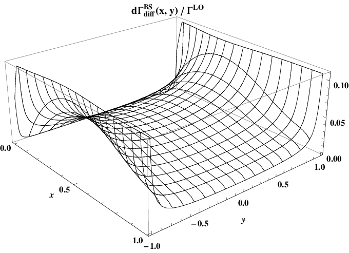

The differential decay rate (cf. (24)) give rise to IR divergences when integrated over the phase space. The divergences originate from the soft-photon region
| (26) |
which is defined in terms of the variables by means of the cut on the Dalitz variable . These divergences are exactly the same as those stemming from an analogous integral of the differential decay rate calculated within the soft-photon approximation. The latter is already included in the two-loop result [3], we therefore present our result for the exact BS as a difference
| (27) |
the integral of which is IR finite. The result for is shown in Fig. 4 and (integrated over the allowed region of given by (22)) in Fig. 5. For we get finally
| (28) |
The dependence of on is shown in Fig. 6. For and for given by (11) we get numerically
| (29) |
where the error stems from the uncertainty in . In other words, using this cut of Dalitz variable in KTeV experiment, the soft-photon approximation is a very good approach to the exact result. The dependence of on is shown in Fig. 7.


Now we have all ingredients needed in formula (16) under control and we can thus fit the value of the coupling to meet the experiment with the result
| (30) |
The error is dominated by the experimental uncertainty, while the theoretical error corresponding to the estimate (13) is negligible. To compare, some previously estimated values, which were considered as relevant, are shown in Tab. 1.
5 Estimate of the theoretical uncertainty of
The above determination of represents an effective LO value of this coupling and includes therefore implicitly higher order chiral contributions. The corrections to the LO value of start at the NLO and stem from the two-loop graphs which correspond to a substitution of the one-loop subgraphs (and corresponding counterterms) for the shaded blob on the left hand side of the graphical equation depicted in Fig. 1. The relative size of such corrections is set by the factor and can be naively treated as negligible, however it can be significantly numerically enhanced by the large double logarithm terms like for .
Complete calculation of the NLO corrections is beyond the scope of the present article. In this section, we will only restrict ourselves to the rough estimate based on explicit calculation of the above mentioned leading (double) logarithms, which are expected to represent a numerically relevant part of the full NLO contribution. According to the Weinberg consistency relation [19], this can be achieved by means of evaluation of infinite parts of one-loop graphs only. In what follows, we will adapt this relation to our case.
Let us write the contribution of the above mentioned two-loop graphs as
| (31) |
where the first three terms correspond to one-particle irreducible (1PI) contributions (including two-loop graphs, one-loop graphs with counterterms and tree counterterm graphs) and the last term represents the renormalization of the external pion line by means of the one-loop -factor. The contributions of the 1PI loop graphs can be written schematically88 8 Because we are interested only in the singular parts we ignore the difference between , and subtraction schemes in what follows. Such an omission can affect only the finite parts which are irrelevant for the leading log calculation. as an expansion in
| (32) |
In the same way, for we get (see Fig. 8)
| (33) |
and the one-loop ingredients of the term are then in the same way (see Fig. 9)
| (34) |
Here , and are finite parts of the one-loop counterterms. We use the standard notation for the two-flavour Chiral Perturbation theory (ChPT) both in the even [20, 21] and in the odd sector [22]. The coefficient can be obtained from (8) and (10)
| (35) |
and will be discussed below. The Weinberg condition is based on absence of nonlocal divergences of the form . It can be expressed as the following constraint
| (36) |
The contribution of the leading double logs is
| (37) |
Using the constraint (36), we get finally
| (38) |
Let us now discuss the ingredients of the formula (38). The infinite parts of the couplings and are
| (39) |
From the finiteness of , it follows
| (40) |
For the couplings , the infinite parts depend on the form of the term in the chiral Lagrangian (see (see [23, 24, 25]) for details). For the standard choice
| (41) |
we get
| (42) |
(in this case, ), while for equivalent case, which differs by terms proportional to the LO equation of motion
| (43) |
we get and
| (44) |
Because both choices have to lead to the same result, we get the following relation
| (45) |
The factor is not a physical observable therefore is both sensitive to the field redefinition and in principle infinite. To calculate it we will use the exponential parametrization (see e.g. [24]):
| (46) |
The only missing ingredients are then , and , which correspond to the one-loop graphs depicted in the Fig. 8. Explicitly, we get
| (47) | ||||
| (48) | ||||
| (49) |
Putting all these ingredients together, we find that
| (50) |
and we get finally
| (51) |
which implies the following leading log correction, which has to be subtracted from the experimentally determined coupling (30)
| (52) |
Numerically
| (53) |
which is well below the uncertainty of in (30). This can be taken as an indication of the robustness of our determination of with respect to the NLO chiral corrections.
6 Conclusion
In this article we have revisited the decay . It has attracted a lot of attention since its recent precise measurement by KTeV Collaboration at Fermilab due to the discrepancy with the theoretical predictions. Provided that the measured quantity is in agreement with the future experiments one can attribute the existing discrepancy to the quantum corrections, correct modeling of the double off-shell pion transition form factor and/or possible contribution of the new physics. Our focus here was on the first part, i.e. standard model corrections to the leading order calculation. We have first briefly summarized recent precise theoretical works dealing with the two-loop QED corrections. The missing bremsstrahlung contribution to this process has been calculated. We have shown that the soft-photon approximation is an adequate approach in the region of KTeV experiment. Besides the electromagnetic corrections we have also studied possible stability in the strong sector. It is best modeled using the higher pion-loop contributions for example in the framework of ChPT. It is often the case that in the two-flavour ChPT the order of these corrections can be estimated by the size of the chiral logarithms. In fact they represent the potential enhancement of the usual counting. We have explicitly calculated the coefficient of the leading logarithm and due to the large suppression factor (see (51)) it turns out to be very small. This might be an indication of the fast convergence of the perturbation series which is a situation similar to the chiral corrections of decay (cf. [25, 26]).
Using the most reliable QCD modeling of the via the lowest-meson dominance approach [13] we agree with the estimate made in [3] of discrepancy between the theory (including all radiative corrections) and the experiment. Let us remind that this number is significantly smaller than usually quoted difference (), however, let us stress that this bigger number was obtained from the rough estimates of the QED radiative corrections and it is thus an indication of the importance of the full two-loop calculation for this process.
On the other hand, still unsatisfactory situation in the first-principle modeling of the three-point vector-vector-pseudoscalar correlator leads to the possibility to use the precise measurement and the full radiative calculation of this process to set the hadronic form factor, represented for this process by the constant . The obtained value (see (30)) is slightly different from the usual estimations, however, represents the model independent prediction for this quantity, based on the KTeV experiment. It can be further used e.g. in the hadronic light-by-light contribution of the muon (see e.g. [27, 28] for details).
Acknowledgment
This work is supported by Charles University in Prague, project PRVOUK P45, and by Ministry of Education of the Czech Republic, grant LG 13031. T.H. was supported by the grants SVV 260097/2014 and GAUK 700214.
Appendix A Explicit form of the bremsstrahlung formfactors
In Section 4 we have defined the invariant amplitude for the bremsstrahlung correction using the form factors , and . In this appendix we will summarize their explicit form using the standard Passarino-Veltman scalar one-loop integrals , and . The only divergent function is then . Its explicit form will be given here as a reference point for our notation
| (54) |
where we have introduced . Note that in this regularization scheme the bare counterterm coupling is given by [29, 13]
| (55) |
The bremsstrahlung form-factors are
| (56) |
| (57) |
| (58) |
In these formulae we have denoted and , i.e.
| (59) |
The real parts of all scalar one-loop integrals used in the previous formulae can be found in [14]. We will list the scalar functions here together with the correct imaginary part:
| (60) |
| (61) |
| (62) |
| (63) |
where , ,
| (64) |
Finally, the four-point function presented in the above formula is given by
| (65) |
where and
| (66) |
References
- [1] A. E. Dorokhov, M. A. Ivanov, Rare decay : Theory confronts KTeV data, Phys. Rev. D75 (2007) 114007. arXiv:0704.3498.
- [2] A. Dorokhov, Rare decay as a Test of Standard Model, Phys. Part. Nucl. Lett. 7 (2010) 229–234. arXiv:0905.4577.
- [3] P. Vasko, J. Novotny, Two-loop QED radiative corrections to the decay : The virtual corrections and soft-photon bremsstrahlung, JHEP 1110 (2011) 122. arXiv:1106.5956.
- [4] S. Drell, Direct decay , Il Nuovo Cimento Series 10 11 (1959) 693–697. doi:10.1007/BF02732327.
- [5] E. Abouzaid, et al. (KTeV Collaboration), Measurement of the rare decay , Phys. Rev. D75 (2007) 012004. arXiv:hep-ex/0610072.
- [6] J. Beringer, et al. (PDG), Review of Particle Physics, Phys. Rev. D86 (2012) 010001. doi:10.1103/PhysRevD.86.010001.
- [7] Bergström, L., Radiative corrections to pseudoscalar meson decays, Z. Phys. C20 (1983) 135–140. doi:10.1007/BF01573215.
- [8] H. Behrend, et al. (CELLO Collaboration), A measurement of the , and electromagnetic form factors, Z. Phys. C49 (1991) 401–410. doi:10.1007/BF01549692.
- [9] J. Gronberg, et al. (CLEO Collaboration), Measurements of the meson-photon transition form factors of light pseudoscalar mesons at large momentum transfer, Phys. Rev. D57 (1998) 33–54. arXiv:hep-ex/9707031.
- [10] A. Dorokhov, E. Kuraev, Y. Bystritskiy, M. Secansky, QED radiative corrections to the decay , Eur. Phys. J. C55 (2008) 193–198. arXiv:0801.2028.
- [11] Y. Kahn, M. Schmitt, T. M. Tait, Enhanced rare pion decays from a model of MeV dark matter, Phys. Rev. D78 (2008) 115002. arXiv:0712.0007.
- [12] M. Knecht, A. Nyffeler, Resonance estimates of low-energy constants and QCD short distance constraints, Eur. Phys. J. C21 (2001) 659–678. arXiv:hep-ph/0106034.
- [13] M. Knecht, S. Peris, M. Perrottet, E. de Rafael, Decay of pseudoscalars into lepton pairs and large- QCD, Phys. Rev. Lett. 83 (1999) 5230–5233. arXiv:hep-ph/9908283.
- [14] K. Kampf, M. Knecht, J. Novotny, The Dalitz decay revisited, Eur. Phys. J. C46 (2006) 191–217. arXiv:hep-ph/0510021.
- [15] J. Wess, B. Zumino, Consequences of anomalous Ward identities, Phys.Lett. B37 (1971) 95. doi:10.1016/0370-2693(71)90582-X.
- [16] E. Witten, Global Aspects of Current Algebra, Nucl.Phys. B223 (1983) 422–432. doi:10.1016/0550-3213(83)90063-9.
- [17] P. Frampton, Conditions for Renormalizability of Quantum Flavor Dynamics, Phys. Rev. D20 (1979) 3372. doi:10.1103/PhysRevD.20.3372.
- [18] G. Passarino, M. Veltman, One-loop corrections for annihilation into in the Weinberg model, Nucl. Phys. B160 (1979) 151–207. doi:10.1016/0550-3213(79)90234-7.
- [19] S. Weinberg, Phenomenological Lagrangians, Physica A96 (1979) 327. doi:10.1016/0378-4371(79)90223-1.
- [20] J. Gasser, H. Leutwyler, Chiral Perturbation Theory to One Loop, Annals Phys. 158 (1984) 142. doi:10.1016/0003-4916(84)90242-2.
- [21] J. Gasser, H. Leutwyler, Chiral Perturbation Theory: Expansions in the Mass of the Strange Quark, Nucl.Phys. B250 (1985) 465. doi:10.1016/0550-3213(85)90492-4.
- [22] J. Bijnens, L. Girlanda, P. Talavera, The Anomalous chiral Lagrangian of order , Eur.Phys.J. C23 (2002) 539–544. arXiv:hep-ph/0110400.
- [23] B. Ananthanarayan, B. Moussallam, Electromagnetic corrections in the anomaly sector, JHEP 0205 (2002) 052. arXiv:hep-ph/0205232.
- [24] K. Kampf, J. Novotny, Effective vertex for , Acta Phys. Slov. 52 (2002) 265. arXiv:hep-ph/0210074.
- [25] K. Kampf, B. Moussallam, Chiral expansions of the lifetime, Phys. Rev. D79 (2009) 076005. arXiv:0901.4688.
- [26] J. Bijnens, K. Kampf, S. Lanz, Leading logarithms in the anomalous sector of two-flavour QCD, Nucl.Phys. B860 (2012) 245–266. arXiv:1201.2608.
- [27] M. Ramsey-Musolf, M. B. Wise, Hadronic light by light contribution to muon g-2 in chiral perturbation theory, Phys.Rev.Lett. 89 (2002) 041601. arXiv:hep-ph/0201297.
- [28] J. P. Miller, E. d. Rafael, B. L. Roberts, D. Stöckinger, Muon (g-2): Experiment and Theory, Ann.Rev.Nucl.Part.Sci. 62 (2012) 237–264. doi:10.1146/annurev-nucl-031312-120340.
- [29] M. J. Savage, M. E. Luke, M. B. Wise, The Rare decays , and in chiral perturbation theory, Phys.Lett. B291 (1992) 481–483. arXiv:hep-ph/9207233.