Dipartimento di Matematica e Fisica, Università di Roma Tre, I.N.F.N. Sezione Roma Tre, Roma, Italy \PACSes\PACSit14.80.Bn14.65.jk
The role of the top quark in the stability of the SM Higgs potential
Abstract
I discuss the stability of the SM scalar potential in view of the discovery of a Higgs boson with mass around 125 GeV. The role played by the top quark mass in the choice between the full stability and the metastability conditions is analyzed in detail. The present experimental value of the top mass do not support the possibility that the SM potential is stable up to the Planck scale but favor an electroweak vacuum sufficiently long-lived to be metastable.
1 Vacuum stability analysis
With the discovery at the LHC of a new resonance [1] with mass around 125-126 GeV and properties very compatible to those of the Standard Model (SM) Higgs boson the complete particle spectrum of the SM is now known. The first run of the LHC has delivered two important messages: i) no signal of physics beyond the SM (BSM) was discovered. ii) The Higgs boson was found where predicted by the SM.
 |
In fig.1 I show the probability density function for the SM Higgs boson mass obtained combining the information from precision measurements with the results of the Higgs search experiments, the latter expressed in terms of the likelihood of the search experiment normalized to the no-signal case [2]. In the figure only the experimental results from LEP and Tevatron before the turning on of the LHC are used. As shown from the figure the SM had a sharp prediction: the mass of the Higgs boson had to be between 114 and 160 GeV. Indeed the Higgs boson was found by ATLAS and CMS exactly in that interval.
The fact that all the parameters of the SM have been now experimentally determined constrains tightly the model and possibly BSM physics. New Physics (NP), if exists, should be of the decoupling type, i.e. it should have a marginal effect on the SM electroweak fit without spoiling its very good agreement with the experimental results. This fact, together with the negative result of the run I of the LHC, may put some doubts on the expectation that NP has to be “around the corner”, i.e. within the reach of the LHC. In this situation it is natural to ask where the scale of NP is, or if it can be as large as the Planck scale, , implying that the validity of the SM can be extended up to .
One approach to answer this question is to study the stability of the SM vacuum, or if the electroweak (EW) minimum we live in is the true minimum of the SM effective potential, i.e. the radiatively corrected scalar potential. The effective potential, in first approximation, has the the same form as the tree-level one but with running parameters ( is the renormalization scale)
| (1) |
then if we are looking at large values of the Higgs field, where is the EW minimum, the dominant contribution to the potential is from the quartic term.
The search for the scale where becomes smaller than its value at the EW minimum, i.e. the instability scale , can be replaced, given the steepness of the potential around that point, by looking for the scale where or, for large values of the field, where . The Higgs quartic coupling is special among the SM couplings. Indeed is the only SM coupling that is allowed to change sign during the Renormalization Group (RG) evolution because it is not multiplicatively renormalized. For all other SM coupling the functions are proportional to their respective couplings and crossing zero is not possible. In fact, one finds for at the one loop level
| (2) |
where is the color factor of , the top Yukawa coupling and and the and gauge couplings, respectively. In the r.h.s. of eq. 2 the part not proportional to contains the top Yukawa coupling at the fourth power and with a negative sign. Thus, for small values of this is the term dominating and is going to evolve towards smaller values eventually crossing zero.

In fig.2 (left) the evolution in the SM of the gauge, Yukawa and scalar couplings is shown. The running of the various couplings has been determined using the state-of-the-art computations, i.e. three-loop beta functions [3] and two-loop matching conditions [4, 5]. The three gauge couplings and the top Yukawa coupling remain perturbative and are fairly weak at high energy, becoming roughly equal, within 10%, around a scale of about GeV. It is amusing to note that the ordering of the coupling constants at low energy is completely overturned at high energy with the (GUT normalized) hypercharge coupling being the largest coupling. The evolution of is zoomed in the right part of fig.2. The Higgs quartic coupling remains weak in the entire energy domain below . It decreases with energy crossing , for the central values of top mass, , the strong coupling, , and the Higgs mass, , at a scale of about GeV.
The fact that becomes negative at a scale lower than is a signal that the effective potential is unstable, i.e. at high scale is either not bounded from below or it develops a second minimum that can be deeper than the EW one. In both cases the idea that the SM can be considered a valid theory up to is in trouble because is no longer the true minimum of the potential and there is a tunnelling probability between the false vacuum and the true vacuum at high field values. However, we can infer that NP must appear below to cure the instability of the SM potential only if the lifetime of EW vacuum is shorter than the life of the universe.
The rate of quantum tunnelling out of the EW vacuum, given by the probability of nucleating a bubble of true vacuum within a space volume and time interval , was first computed in the late seventies by S. Coleman [6]. The total probability for vacuum decay to have occurred during the history of the universe can be computed by integrating over the space-time volume of our past light-cone, or
| (3) |
where is the age of the universe and is the action of the bounce of size . is determined as the scale at which is maximized [7]. In practice this roughly amounts to minimizing , which corresponds to the condition . By numerical inspection of in eq.(3) one finds that the exponential suppression wins over the large 4-volume factor if is less than .
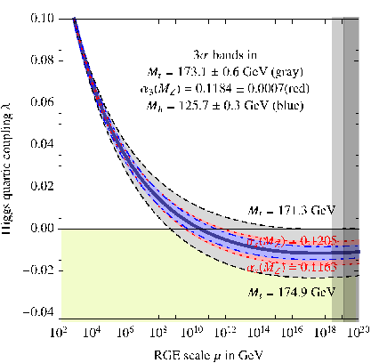
Fig.2 shows that in its RG evolution towards does become negative but never too negative. In fact the running of is slowing down at high energy because its function at high scale becomes very small, vanishing close to . At the Planck scale one then finds [5]
| (4) | |||||
that implies that our vacuum is metastable, i.e. is extremely small (less than ) or the lifetime of the EW vacuum is extremely long much larger than .
  |
The study of the two-loop effective potential [8] allows us to identify the phases of the SM. They are shown in fig.3 as a function of the Higgs and top masses. The regions of stability, metastability, and instability of the EW vacuum are shown both for a broad range of and , and after zooming into the region corresponding to the measured values. The uncertainty from and from theoretical errors is indicated by the dashed lines and the color shading along the borders. Also shown are contour lines of the instability scale. The measured values of and appear to be rather special, in the sense that they place the SM vacuum at the border between stability and metastability. In the neighborhood of the measured values of and , the stability condition is well approximated by
| (5) |
Since the experimental error on the Higgs mass is already fairly small and will be further reduced by future LHC analyses, it is becoming more appropriate to express the stability condition in terms of the pole top mass or
| (6) |
2 The role of the top quark
As is clear from the right plot in fig.3, it is the exact value of the top mass, rather than a further refined computation, the factor that can discriminate between a stable and a metastable EW vacuum. Fig.3, as well as the bound (6), are obtained using as renormalized mass for the top quark the so-called pole mass and identifying it with the average of the Tevatron, CMS and ATLAS measurements, GeV. This identification can be disputed in two aspects. i) From a theoretical point the concept of pole mass for a quark is not well defined as quarks are not free asymptotic states. Furthermore the quark pole mass is plagued with an intrinsic non-perturbative ambiguity of the order of due to the so-called infrared (IR) renormalon effects. ii) The top mass parameter extracted by the experiments, which we call , is an object that is obtained via the comparison between the kinematical reconstruction of the top quark decay products and the Monte Carlo simulations of the corresponding event. The latter requires a careful modeling of the jets, missing energy, initial state radiation contributions as well as of the hadronization part. is a parameter sensitive to the on-shell region of the top quark but it cannot be directly identified with the pole mass. We can write generically with the understanding that the error quoted by the experimental collaborations refers to and not to . The point now is what is the size of . An analysis of the phase-space regions in the top production cross-section at hadron colliders shows that the region possibly sensitive to IR effects contributes very little to the total rate. Then, even assuming an uncertainty of 100 % in the modelling of that region, the extraction of from the total rate will be affected only at the level of MeV. Thus we can conclude that can be interpreted as within the intrinsic ambiguity in the definition of , that implies MeV [9].
It is well known that short distance masses, such the one defined in the scheme, do not suffer from the IR renormalon problem. The top mass, , can be extracted directly from the total production cross section for top quark pairs . A recent analysis reports [10], a value that translated in terms of pole mass gives for a central value very close to that obtained via the decay products but a much larger error
| (7) |
The use of masses in the EW theory requires some specification. Differently from QCD, in the EW theory masses, as well as , are not parameters of the EW Lagrangian. The parameters are the gauge, Yukawa and the scalar couplings. This implies that the definition of an mass is not unique: it depends upon the definition of the vacuum. Indeed we can define the vacuum either as the minimum of the tree-level scalar potential or as the minimum of the radiatively corrected potential. In the first case we get an mass that is gauge invariant, but there will be large EW corrections in the relation between the pole and the mass [11]. In the case of the top quark they are proportional to implying that if we want to extract directly from we have to consider the EW radiative corrected cross section. In the second case, when the vacuum is defined via the corrected potential, these large corrections are absent however the resulting mass is not a gauge-invariant object. Although this fact can seem quite awkward we should remember that an mass is not a physical object and therefore gauge invariance is not a mandatory requirement.
 |
It is clear that, because is determined with an error much larger than that of its use in the analysis of vacuum stability will weaken the conclusion that the EW vacuum is metastable while admitting, within in the top mass error, the possibility of full stability. However, we can take a different point of view: the top pole mass is the same object that enters the EW fit and it can be predicted now that we know the Higgs mass quite accurately. Is the value obtained from the fit compatible with the bound (6)? The answer is in fig.4 where the probability density function for is shown with the dark (light) region corresponding to interval. From the figure it is clear that values of around GeV are in the tail of the distribution with a probability of few per cent.
3 Conclusions
The SM is in a very good status. The value of the Higgs mass found by ATLAS and CMS is very intriguing. It causes the SM potential to be at the border of the stability region. The exact value of the top mass plays the central role between the full stability or the metastability (preferred) options. The possibility of up to requires a top mass value around GeV, a number not preferred by the EW fit. Finally, the fact that our EW vacuum is metastable with a lifetime much longer than the age of the universe does not allow us to conclude that NP must appear at a scale lower than the Planck scale.
Acknowledgements.
I would like to thank the organizers of LC13 for their kind invitation. I am in debt with all the people I have collaborated with on this subject: D. Buttazzo, S. Di Vita, J. Elias-Miró, J.R. Espinosa, P.P. Giardino, G. Giudice, G. Isidori, F. Sala, A. Salvio and A. Strumia. Interesting discussions with F. Maltoni and P. Slavich are also acknowledged. This work was partially supported by the Research Executive Agency (REA) of the European Union under the Grant Agreement number PITN-GA- 2010-264564 (LHCPhenoNet).References
- [1] \BYAad G.et al. [ATLAS Collaboration] \INPhys. Lett. B71620121 [arXiv:1207.7214]; \BYChatrchyan S.et al. [CMS Collaboration] \INPhys. Lett. B716201230 [arXiv:1207.7235].
- [2] \BYD’Agostini G. \atqueDegrassi G. \INEur. Phys. J. C 101999663 [hep-ph/9902226].
- [3]
\BYTarasov O.V. Vladimirov A.A. \atqueZharkov A.Y.
\INPhys. Lett. B 931980429;
\BY Larin S.A. \atqueVermaseren J.A.M. \INPhys. Lett. B 3031993334 [hep-ph/9302208];
\BYMihaila L.N. Salomon J. \atqueSteinhauser M. \INPhys. Rev. Lett. 1082012151602 [arXiv:1201.5868], \INPhys. Rev. D 862012096008 [arXiv:1208.3357];
\BY Chetyrkin K.G. \atqueZoller M.F. \INJHEP 12062012033[arXiv:1205.2892] ;
\BYBednyakov A.V. Pikelner A.F. \atqueVelizhanin V.N. \INPhys. Lett. B 7222013336 [arXiv:1212.6829]. - [4] \BYBezrukov F. Kalmykov M.Y. Kniehl B.A. \atqueShaposhnikov M. \INJHEP 12102012140 [arXiv:1205.2893].
- [5]
\BYDegrassi G. Di Vita S. Elias-Miro J. Espinosa J.R. Giudice G. Isidori G.
\atqueStrumia A.
\INJHEP 12082012098 [arXiv:1205.6497];
\BYButtazzo D. Degrassi G. Giardino P.P. Giudice G. Sala F. Salvio A. \atqueStrumia A. \INJHEP 13122013089 [arXiv:1307.3536]. - [6] \BYColeman S.R. \INPhys. Rev. D 1519972929 [Erratum-ibid. D 16 (1977) 1248];
- [7] \BYIsidori G. Ridolfi G. \atqueStrumia A. \INNucl. Phys. B6092001387 [hep-ph/0104016]
- [8]
\BYFord C. Jack I. \atqueJones D.R.T.
\INNucl. Phys. B3871992373
[Erratum ibid. \SAME5041997 551] [hep-ph/0111190];
\BYMartin S.P. \INPhys. Rev. D652002116003 [hep-ph/0111209]. - [9] \BYMangano M. \TITLEtalk given at the TOP 2013 Conference, Durbach September 14-19 2013.
- [10] \BYAlekhin S. Djouadi A. \atqueMoch S. \INPhys. Lett. B 7162012214 [arXiv:1207.0980].
- [11] \BYJegerlehner F. Kalmykov M.Y. \atqueKniehl B.A. \INPhys. Lett. B 722 2013123 [arXiv:1212.4319].