Post-Sphaleron baryogenesis and oscillation in non-SUSY GUT with gauge coupling unification and proton decay
Abstract
Post-sphaleron baryogenesis”, a fresh and profound mechanism of baryogenesis accounts for the matter-antimatter asymmetry of our present universe in a framework of Pati-Salam symmetry. We attempt here to embed this mechanism in a non-SUSY SO(10) grand unified theory by reviving a novel symmetry breaking chain with Pati-Salam symmetry as an intermediate symmetry breaking step and as well to address post-sphaleron baryogenesis and neutron-antineutron oscillation in a rational manner. The Pati-Salam symmetry based on the gauge group is realized in our model at GeV and the mixing time for the neutron-antineutron oscillation process having is found to be with the model parameters which is within the reach of forthcoming experiments. Other novel features of the model includes low scale right-handed , gauge bosons, explanation for neutrino oscillation data via gauged inverse (or extended) seesaw mechanism and most importantly TeV scale color sextet scalar particles responsible for observable oscillation which can be accessible to LHC. We also look after gauge coupling unification and estimation of proton life-time with and without the addition of color sextet scalars.
I INTRODUCTION
The Standard Model (SM) of particle physics has given us enough reasons to look beyond its framework for dealing with issues like tiny neutrino masses, matter-antimatter asymmetry of the present universe, Dark matter and Dark energy, coupling unification of three fundamental interactions. Among all these, the observed baryon asymmetry of the universe has motivated the scientific community to work upon it since a long time. The WMAP satellite data [1, 2], when combined with large scale structures (LSS) data, gives the baryon asymmetry of the universe to be while an independent measurement of baryon asymmetry carried out by BBN [3] yields . Two compelling mechanisms namely Leptogenesis [4] and Weak scale baryogenesis [5] have been prime tools for explaining baryon asymmetry of the universe. In leptogenesis the desired lepton asymmetry is created by the lepton number violating as well as out of equilibrium decays of heavy particles which is subsequently converted into baryon asymmetry by the non-perturbative ()-violating sphaleron interactions [6, 7].
An inadequate knowledge about the nature of new physics beyond the standard model leaves us with no choice but to explore all possibilities which may explain the origin of matter-antimatter asymmetry. Recently a new idea behind baryon asymmetry has been explored named ”Post-Sphaleron baryogenesis (PSB)” which occurs via the decay of a scalar boson singlet under standard model having mass around few hundreds of GeV and a high dimensional baryon number violating coupling [10, 8, 9], where the Yukawa coupling(s) of the scalar(s) act as the source of CP-asymmetry. Apparently,this high dimensional baryon number violating coupling is generated via new physics operative beyond standard model electroweak theory. The mechanism of PSB is based on the idea that the required amount of baryon asymmetry of the universe can be generated below the scale of electroweak phase transition where the sphaleron has decoupled from the Hubble expansion rate. Although the proposal seems interesting it has not yet been incorporated in a realistic grand unified theory. Hence we attempt here to embed the proposal of PSB in a non-SUSY SO(10) GUT with Pati-Salam (PS) symmetry and Left-Right (LR) symmetry as intermediate symmetry breaking steps.
A detail study of the literatures [11, 12, 13, 14, 15, 16, 17, 18] gives an idea about many intriguing features of the grand unified theory (including both non-SUSY and SUSY). One of these features is that when left-right gauge symmetry appears as an intermediate symmetry breaking step in a novel symmetry breaking chain, then seesaw mechanism can be naturally incorporated into it. In conventional seesaw models associated with thermal leptogenesis the mass scale for heavy RH Majorana neutrino is at GeV which makes it unsuitable for direct detectability at current accelerator experiments like LHC. Therefore, it is necessary to construct a theory having and gauge groups as intermediate symmetry breaking steps which results in low mass right-handed Majorana neutrinos along with , gauge bosons at TeV scale. At the same time it should be capable of explaining post-sphaleron baryogenesis elegantly along with other derivable predictions like proton decay and neutron-antineutron oscillation.
We intend to discuss TeV scale post-sphaleron baryogenesis, neutron-antineutron oscillation having mixing time close to the experimental limit with the Pati-Salam symmetry or GUT as mentioned in a recent work [19] slightly modifying the Higgs content where non-zero light neutrino masses can be accommodated via gauged extended inverse seesaw mechanism along with TeV scale , gauge bosons. As discussed in the work [19] the Dirac neutrino mass matrix is similar to the up-quark mass matrix even with low scale right-handed symmetry breaking. Though the details has been already discussed in the above mentioned work we breifly clarify the point as follows.
In non-SUSY , the type I seesaw [20] contribution to neutrino mass is given by
where is the Dirac neutrino mass matrix, is the Majorana neutrino mass matrix for right-handed neutrinos and is related to the right-handed symmetry breaking scale. The Dirac neutrino mass matrix and up-quark mass matrices are similar in a generic model that has high scale Pati-Salam symmetry as an intermediate breaking step relating quarks and leptons with each other. Hence, , which further implies that the neutrino Dirac Yukawa coupling should be equal to top-quark Yukawa coupling. With GeV, the sub-eV scale of light neutrino consistent with oscillation data requires the right-handed scale (seesaw scale) to be greater than GeV. Such high seesaw scale makes this idea difficult to be probed at any foreseeable laboratory experiments. Hence, as an alternative way, emphasizing on its verifiability at LHC, inverse seesaw mechanism [21, 22] has been proposed, with an extra fermion singlet (in addition to the existing fermion content of ), with light neutrino mass formula
where is the mixing matrix and is the small lepton number violating mass term for sterile neutrino . The above relation can be recasted as
Hence, sub-eV mass for light neutrinos are consistent with (or, ) which is a generic predictions of high scale Pati-Salam symmetry and compatible with low right-handed symmetry breaking scale () since inverse seesaw formula is independent of . We have utilised this particular property of low scale right-handed symmetry breaking in studying Post-sphaleron baryogenesis and neutron-antineutron oscillation even though a complete discussion on the origin of neutrino masses and mixing via low sacle extended inverse seesaw has been omitted.
Here we sketch out the complete work of our paper. In Sec.II, we briefly discuss non-SUSY GUT with a novel symmetry breaking chain, having and as intermediate symmetry breaking steps. In Sec.III we show how gauge coupling unification is achieved in our model. In Sec.IV we discuss the TeV scale post-sphaleron baryogenesis and embed it within the novel chain of non-SUSY model with the self-consistent model parameters. In Sec.V, we estimate the mixing time for neutron-antineutron oscillation. In Sec.VI, we present an idea how low mass scales for RH Majorana neutrino as well as right-handed gauge bosons , are allowed in the model, while explaining light neutrino masses via gauged extended seesaw mechanism. In Sec.VII we conclude our work with results and summary including a note on viability of the model at LHC.
II THE MODEL
In this section we shall discuss the one-loop gauge coupling unification and estimate the proton life time including short distance enhancement factor to the proton decay operator by reviving the symmetry breaking chain [19]
| (1) | |||||
The chain breaks in a sequence, where first breaks down to after the Higgs representation is given a VEV, then the spontaneous breakdown of D-parity occurs in with the assignment of VEV to D-parity odd component contained in the Higgs representation . The decomposition of under is
| (2) | |||||
Spontaneous D-parity mechanism is aptly utilized here, since the theory allows low mass scale for right-handed Higgs fields around (TeV) while keeping all its left-handed components at D-parity breaking scale. Now assigning a VEV to the neutral component , the Pati-Salam symmetry () breaks down to left-right symmetry (). The next step of symmetry breaking occurs via the VEV . The right-handed gauge boson acquires a mass in the range of few TeV and contributes sub-dominantly to neutrinoless double beta decay.
The most desirable symmetry breaking step is achieved by the of though we have added another Higgs representation for realization of gauged inverse seesaw mechanism operative at TeV scale. The decomposition of the Higgs under is
As we have pointed earlier, due to D-parity mechanism, the right-handed triplet Higgs field contained in gets its mass at TeV scale while its left-handed partner has its mass at D-parity breaking scale . As a result of this symmetry breaking, the neutral component of right-handed gauge boson gets its mass around (TeV) with the experimental bound TeV [25, 24]. The final stage of symmetry breaking is carried out by giving VEV to the neutral component of SM Higgs doublet contained in the bidoublet .
We shall now check whether having TeV scale post-sphaleron baryogenesis, neutron-antineutron oscillation and gauged inverse seesaw mechanism is consistent with gauge coupling unification. It is found that the coupling constants unify at () GeV with the Higgs fields + + + +. Some good reasons behind taking these Higgs fields are; firstly, the TeV scale post-sphaleron baryogenesis and neutron-antineutron oscillation can be well explained with these parameters while predicting gauge boson in TeV range; secondly, it allows breaking () at TeV scale resulting mass TeV, moreover it explains tiny masses for light neutrinos consistent with neutrino oscillation data via TeV scale gauged inverse seesaw mechanism and LFV decays with branching ratios accessible to ongoing search experiments.
III GAUGE COUPLING UNIFICATION AND PROTON DECAY
III.1 One-loop renormalization group equations (RGEs) for gauge coupling evolution
For simplicity, we consider only the one-loop renormalization group equations(RGEs) for gauge coupling evolution which can be written as
| (4) |
where, , is the fine structure constant, and is the one-loop beta coefficients derived for the the corresponding gauge group for which coupling evolution has to be determined. Using the input parameters, electroweak mixing angle , electromagnetic coupling constant and strong coupling constant taken from PDG [3, 23] the values of three coupling constants at electroweak scale GeV can be calculated precisely to be,
| (5) |
where denote the fine structure constants for the SM gauge group .
III.2 Higgs content for the model and corresponding one-loop beta coefficients
The Higgs contents for the model used in different ranges of mass scales under respective gauge symmetries () with a particular symmetry breaking chain as considered in a recent work [19] where the prime interest was to keep the , gauge bosons at TeV scale are as follows,
| (6) |
| (7) |
Here we find two categories of Higgs spectrum; Model-I having Higgs spectrum as given in eqn.( 6) and eqn.( 7) excluding the bitriplet Higgs scalar which estimates a proton life time that is far from the reach of search experiments and Model-II having the same Higgs spectrum, including the bitriplet Higgs scalar from mass scale onwards which estimates a proton life time very close to the experimental limit. Thus Model-II serves our purpose.
The one-loop beta coefficients are found to be the same for both the models at mass scale ranges , , and i.e.,
| (8) |
whereas, they differ at Pati-Salam scale to the Unification scale as shown in Table.1.
| Mass ranges | for Model-I | for Model-II | |
|---|---|---|---|


The gauge coupling unification for this work is shown in Fig. 1 with the allowed mass scales desirable for our model predictions,
| (9) |
III.3 Estimation of Proton life time for
The decay rate for the gauge boson mediated proton decay in the channel including strong and electroweak renormalization effects on the operator starting from the GUT scale to the proton mass (i.e, 1 GeV) [26, 27] comes out to be
| (10) |
In the eq. (10), is renormalization factor from the electroweak scale to the proton mass, , , , and which have been extracted as phenomenological parameters by the chiral perturbation theory and lattice gauge theory. Also is the proton mass, and is the gauge fine structure constant derived at the GUT scale. It is worth to note here that the renormalization factor for , with being the short-distance renormalization factor in the left (right) sectors, and is the element of for quark mixings.
After re-expressing , and , the proton life time can be expressed as
| (11) |
where .
Short distance enhancement factor extrapolated from GUT scale to GeV: For estimating proton decay rate in the channel having dimension-6 operator, one needs to extrapolate the operator from the GUT scale physics to the low energy physics at the scale of [28, 29, 30]. With the particular symmetry breaking chain allowed in the non-SUSY model (following the ref. [30]), the whole energy range can be separated into following parts
-
from non-SUSY GUT scale,, to the Pati-Salam symmetry with D-parity (, ) invariance scale, ,
-
from to the Pati-Salam symmetry without D-parity (, ) scale ,
-
from to breaking scale, , where we have left-right symmetric model (LRSM) ,
-
from left-right symmetry breaking scale () to scale ()
-
from scale () to standard model ,
-
from standard model to .
As discussed in refs. [28, 29, 30], the enhancement factor below SM for the operator is
where, denotes the number of quark flavors at the particular energy scale of our interest. Neglecting the effect due to and since their contributions are suppressed as compared to the strong coupling effect , this enhancement factor can be expressed in a more explicit manner as
| (12) |
Since the model considered here is non-supersymmetric version of GUT, all other enhancement factors can be written in the same way as
| (13) |
with () as the anomalous dimension (one-loop beta coefficients) for the corresponding gauge group . Similarly, one can write the enhancement factor valid for , , , and as
Hence, the complete short distance enhancement renormalization factor for this proton decay operator is found to be
| (14) |
We have earnestly followed the prescription given in ref.[28, 29] for the derivation of anomalous dimension for the effective proton decay operator. With a choice of TeV scale particle spectrum used in our model, the unification scale is found to be GeV for Model-I and GeV for Model-II. We have estimated the factor , approximately, to be with the value of long distance renormalization factor which is the same for both the models.
IV TEV SCALE POST-SPHALERON BARYOGENESIS
IV.1 Basic interaction terms
As already discussed in Sec. III, Pati-Salam symmetry survives till few TeV scale playing an important role in the explanation of baryogenesis mechanism and neutron-antineutron oscillation. We need to know all the basic interactions using quarks and di-quarks under high scale Pati-Salam symmetry as well as under low scale SM like interactions around TeV scale in order to explain the above said phenomena successfully. For that, we take a look at the decomposition of the Pati-Salam Higgs representation under left-right symmetry group and the SM gauge group
| (18) | |||||
where the electric charge is expressed in terms of the generators of the SM group and left-right symmetric group as,
| (19) |
Since the fields , , , and quark fields are mainly responsible for non-zero baryon asymmetry and neutron-antineutron oscillation,we need to know the exact interactions among them. The desirable interaction Lagrangian for diquark Higgs scalars with the SM quarks at TeV scale which will yield observable neutron-antineutron oscillation and post-sphaleron baryogenesis is
| (20) | |||||
where , are the Majorana couplings and is the generator for group.
Within the framework, the Yukawa couplings obey the boundary condition, in the limit and the same holds true for quartic Higgs couplings as well. All fermions are right-handed (when chiral projection on the operator is suppressed) and a fermion field under the high scale Pati-Salam symmetry transforms as,
The diquark Higgs scalars transforming under the SM gauge group are denoted with quantum numbers as,
| (24) |
It is clear from eqn (20) that the Higgs field is a neutral complex field. The breaking of is achieved by assigning a VEV to its neutral component . Its real component acquires a VEV in the ground state which can be represented as while the field gets absorbed by the gauge boson corresponding to the gauge group . Therefore, the remaining real scalar field is indeed the physical Higgs particle which serves our purpose of explaining post-sphaleron baryogenesis and neutron-antineutron oscillation.
IV.2 General expression for CP-asymmetry
Without loss of generality, if we consider the particle and antiparticle decay modes of ( being its own antiparticle) i.e, which gives a change of baryon number , and which gives , then the -asymmetry in baryon number produced by these decays can be quantified as,
| (25) |
where is the total decay rate with and . It is evident from eqn (25) that we need divergent partial decay rates for particle and antiparticle decays in order to produce correct amount of baryon asymmetry and hence we should derive the general conditions under which and can be different. It is worth to mention here that the other decay modes of have been ignored for simplicity by adjusting the corresponding couplings involved in the respective decay modes.

In generic situations where the theory is CPT-conserving, there can never be a difference between and if one considers only the tree-level process depicted in Fig. 2 since at tree level. It is found that the nonzero contribution to comes from the interference between the tree-level graph (shown in Fig. 2) and the one-loop corrections (shown in Fig. 3).
IV.3 Constraints on post-Sphaleron baryogenesis
Here we illustrate how post-Sphaleron baryogenesis is slightly different from any other standard baryogenesis process. For post-Sphaleron baryogenesis to be successful in explaining the required matter-antimatter asymmetry of our Universe, few extra conditions must be satisfied by the model parameters along with the Sakharov conditions that says, particle interaction must (i) violate baryon number, , (ii) violate and , and (iii) be out of thermal equilibrium. Firstly, the Higgs scalar should be lighter than other members contained in the Pati-Salam multiplet i.e, the diquark Higgs scalars so that the baryon number conserving decays involving on-shell are kinematically forbidden. Secondly, the out of equilibrium baryon number violating decays should occur after the electroweak phase transition so that it will not be affected by the Sphaleron processes which is proactive at TeV scale. We make it a point here that ref. [9] neatly elaborates the mechanism of post-sphaleron baryogenesis.
IV.4 Out of equilibrium condition
For effectively creating the baryon asymmetry of the universe via post-Sphaleron baryogenesis, the decays of should satisfy the out of equilibrium condition, which is described by where is the total decay width and is the Hubble parameter with the reduced Planck mass and is the number of relativistic degrees of freedom. In order to satisfy the out of equilibrium condition, we should have
| (26) | |||||
To illustrate the mechanism of post-sphaleron baryogenesis, we require extra fields , and as color sextets and singlet scalar bosons that couple to the right-handed quarks contained in the Pati-Salam multiplet . For set of model parameters GeV, GeV, the decoupling temperature is found to be 2 GeV which is well below the EW scale where the Sphaleron has been decoupled. Hence, it is inferred from the above equation that the decay of goes out of equilibrium around . Below this temperature (), the decay rate falls very rapidly as the temperature cools down.

IV.5 Estimation of net baryon asymmetry
Now we concentrate on estimating the CP-asymmetry coming from the interference term between the tree level and the one-loop level diagrams for the decay of which is shown in Fig.2 and Fig.3 respectively. For discussion on baryon number violation in the loop diagram and necessary derivation of the interference diagram, interested readers may go through reference [9]. In the present work, we only check whether or not the representative set of model parameters provide the correct number for the required baryon asymmetry of the universe. Hence, without going deep into the derivation, we simply note here down, the calculated CP-asymmetry for post-sphaleron baryogenesis via decay of with baryon number violating interactions.
| (27) | ||||
| (28) | ||||
| (29) |
Here the expression in eq.(27) represents the CP-asymmetry coming from interference between the tree and one-loop self energy diagram while the expression in eq.(28) represents the CP-asymmetry due to interference of the tree and one-loop vertex diagram (see ref.[9] for details). In the above expression, is the well known CKM matrix in the quark sector, correspond to the up-quark indices while represent to down-quark indices . Sum over repeated indices (Einstein convention) is implicitly assumed here. The is due to the fact that the CP asymmetry is non-zero only when we have a top quark in the final state (since only the CKM elements involving third generation have a large imaginary part).
As mentioned earlier,the mechanism of post-sphaleron baryogenesis provides a natural explanation for the observed baryon asymmetry of our universe i.e, . Using GeV, GeV, GeV, CKM mixing elements and Yukawa couplings relevant for color scalar particles in their allowed range, the CP-asymmetry via the decay of through loop diagrams with the exchanges of bosons is estimated to be . A further dilution of the baryon asymmetry arises from the fact that , since the decay of releases entropy into the universe. As a result the final baryon asymmetry, taking into account the dilution factor, becomes
| (30) |
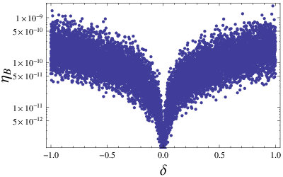
where is the decoupling temperature of the color scalar and is the mass of the scalar. The condition , otherwise leads to suppressed baryon asymmetry, which finally results a baryon asymmetry in the range of . The scatter plot between the final baryon asymmetry including dilution factor () with this phase () is shown in Fig. 4.
V OBSERVABLE NEUTRON-ANTINEUTRON OSCILLATION WITH TEV SCALE DIQUARK HIGGS SCALARS:

V.1 Feynman amplitudes for neutron-antineutron oscillation
We consider the contributions arising only from the RH diquark Higgs fields having masses at TeV scale while ignoring the contributions from LH diquark Higgs fields since they have masses at around eV range. The Feynman diagrams contributing to the neutron-antineutron oscillation are shown in Fig. 5 (loop-diagram), Fig. 6(a) and Fig. 6(b). Our prime goal is to estimate the mixing time for this loop diagram, clarifying why we have suppressed other contributions within our model parameters.
There are two types of contributions to oscillation in the right-handed sector at loop level (i) one involving one -type and two -type, (ii) other one involving one -type and two -type -bosons. The Feynman amplitude for the second type of contribution where one needs to change the two quarks to two quarks from the already generated effective operator via a second order weak interactions (given in Fig. 5) can be written as,
| (31) |
And, the Feynman amplitude for tree level processes shown in Fig. 6(a) and Fig. 6(b) (which are suppressed with the choice of our model parameters), can be written as,
| (32) | |||||


V.2 Prediction for neutron-antineutron mixing time
Before estimating the oscillation mixing time one should carefully fix the input parameters in order to satisfy flavor changing neutral current (FCNC) constraints and to give correct amount of baryon asymmetry of the universe. For example, using diquark sextet Higgs scalar mass around TeV scale, the corresponding Yukawa coupling along with other allowed range of model parameters contradicts the FCNC constraints and hampers post-sphaleron baryogenesis even though it predicts neutron-antineutron oscillation time (as shown in Fig. 6) within the experimental search limits. So this means that one has to choose the Majorana Yukawa coupling accordingly. Now we briefly discuss how this choice of can be achieved within the framework of SO(10) (elaborated in ref [19]).
It is found in ref [19] that all charged fermion masses and CKM mixing can be fitted well at GUT scale within the framework of SO(10) with two kinds of structures; I) with single Higgs representation , II) with two Higgs representations , . As it has been derived, structure-I with Yukawa coupling = diag(0.0236, -0.38, 1.5) estimates oscillation mixing time to be secs which doesn’t serve our purpose. Rather we consider structure-II where the dominant contribution to oscillation comes from the loop diagram while suppressing the tree level contribution. This choice of having two Higgs , not only fits fermion masses at GUT scale, but also allows RH neutrino Majorana mass and hence corresponding Yukawa coupling as per our requirement. Due to the second Higgs representation with its Yukawa coupling to fermions we get MeV following the same procedure, provided all other components are at the GUT scale except which is at the intermediate scale GeV. By treating the mass of to remain at its natural GUT-scale value, its induced VEV is negligible and precision unification with large GUT scale value is unaffected except for phenomenologically inconsequential additional threshold effects. Then defining gives exactly the same fit to the GUT scale fermion masses and mixings but now with the diagonal structure . But since and only with VEV is used to break , the coupling and hence are allowed to have any form without any restriction. In order to suppress the tree level contributions to oscillation as shown in Fig. 6 which otherwise causes problem in baryon asymmetry, we particularly choose the Majorana coupling as per our requirement, i.e, .
| (GeV) | (GeV) | (sec) | ||||
| 0.001 | 0.01 | 0.01 | 0.1 | |||
| 0.001 | 0.01 | 0.01 | 0.1 | |||
| 0.001 | 0.01 | 0.01 | 1 | |||
| 0.001 | 0.001 | 0.001 | 0.1 |
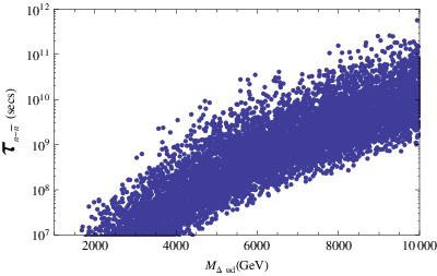
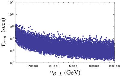
Using this particular choice of Yukawa couplings i.e, and others in the range of , one can calculate the mixing time for neutron-antineutron oscillation as a function of Mass of color Higgs scalar ( breaking scale) as shown in Fig. 7 (Fig. 8).
The amplitude can be translated into the oscillation time as,
| (33) |
with = as used in ref.[9]. The estimated oscillation time for various choice of model parameters i.e, , , B-L breaking scale from (3-5)TeV and the masses of between and , is presented in Table.2.
V.3 Coupling Unification including diquarks at TeV scale
It is prominent that the post-sphaleron baryogenesis and neutron-antineutron oscillation phenomena require existence of color Higgs scalars, having masses around TeV scale. In this subsection, we intend to examine whether unification of gauge couplings is still possible after the addition of extra color scalars , , to the existing particle content as noted in Sec.III, by studying their respective renormalization group equations. The one-loop beta coefficients derived for the present model along with their gauge symmetry groups, range of mass scales and spectrum of Higgs scalars necessary for gauge coupling unification to explain TeV scale post-sphaleron baryogenesis and neutron-anti-neutron oscillation are given below
| (34) | |||
| (35) |
| (36) |
| (37) |
In analogy to the above discussion, we have two scenarios; one without bitriplet and another with bitriplet Higgs scalar (3,3,1) under the Pati-Salam group while its effect has been included from onwards to the unification scale . Accordingly, we have estimated the one-loop beta coefficients for these two scenarios as
| (38) |
| (39) |

The gauge coupling unification after the addition of extra color sextet scalars particles is shown in Fig. 9 with the allowed mass scales desirable for our model predictions,
| (41) |
VI VIABILITY OF THE MODEL
As already known, the lepton flavor and lepton number violating dilepton signals can be probed from the production of heavy RH Majorana neutrino via , from which can be further decayed into . This process, being the main channel for production via on-shell production and fusion, needs to be verified at LHC and our model suits the purpose, since we have , gauge bosons and scalar diquarks at TeV scale. A more pleasant situation is that the model, though non-supersymmetric, predicts similar branching ratios as in supersymmetric models for LFV processes like , , and . And the predicted branching ratios for these LFV decays, being closer to the current experimental search limits can be used to verify the left-right framework in this model. Moreover the estimated neutron-antineutron oscillation mixing time, gauge coupling unification and proton life time in the model stay in the range of ongoing search experiments.
Besides all these points, the model can also predict a number of verifiable new physical quantities like (i) new non-standard contribution to rate in the channel, (ii) contributions to branching ratios of lepton flavor violating (LFV) decays, (iii) leptonic CP-violation due to non-unitarity effects, (iv) experimentally verifiable proton decay modes such as , provided the gauged inverse seesaw mechanism is found to be operative. We find it appropriate to mention here that these physical quantities were also discussed in a recent work [19], but in that model the asymmetric left-right gauge symmetry was incorporated at TeV.
VII CONCLUSION
We have closely studied the mechanism of post-sphaleron baryogenesis, that can potentially explain matter-antimatter asymmetry of the present universe, by analyzing the basic interactions using quarks and diquark Higgs scalars under high scale Pati-Salam symmetry and low scale SM like interactions at TeV scale. The study estimates the total baryon asymmetry to be and neutron-antineutron oscillation with mixing time to be secs which can be accessible at ongoing search experiments. We have made an humble attempt to embed the framework of PSB in a non-SUSY model with Pati-Salam symmetry as a low scale intermediate breaking step where we have shown a strong interlink between post-sphaleron baryogenesis and neutron-antineutron oscillation operative at TeV scale and laid out a novel mechanism of inducing required CP-asymmetry via the SM loops.
More essentially, we have embedded TeV scale LR model within the framework of model where the predicted mass for light neutrinos matches with the neutrino oscillation data. Our calculations indicate that TeV scale masses of and heavy RH neutrinos can also give dominant non-standard contributions to neutrinoless double beta decay which may sound crucial to the experimentalists. Some more good features of the model are explanation of non-zero light neutrino masses via extended/inverse seesaw mechanism, new non-standard contribution to neutrinoless double beta decay, leptonic CP-violation from non-unitary effects.
ACKNOWLEDGEMENT
Sudhanwa Patra would like to thank the organizers of workshop entitled “Majorana to LHC: Origin of neutrino Mass”at ICTP, Trieste, Italy during 2-5 October, 2013 where the idea for this work was conceived. Both the authors sincerely acknowledge P.S. Bhupal Dev for his useful clarification while preparing the manuscript. Prativa Pritimita is grateful to the Department of Science and Technology, Govt. of India for INSPIRE Fellowship (IF140299). The work of Sudhanwa Patra is supported by the Department of Science and Technology, Govt. of India under the financial grant SERB/F/482/2014-15.
References
- [1] J. Dunkley et al. “ WMAP Collaboration,”. arXiv:0803.0586 [astro-ph].
- [2] Komatsu, E. et al “ Seven-Year Wilkinson Microwave Anisotropy Probe (WMAP) Observations: Cosmological Interpretation,”. Astrophys. J. Suppl. 192 (2011) 18 arXiv:1001.4538 [astro-ph].
- [3] W.-M. Yao et al. “Particle Data Group:2006, partial update for edition 2008 (URL: http://pdg.lbl.gov),” J. Phys. G 33, 1 (2006).
- [4] M. Fukugita and T. Yanagida, “Baryogenesis without Grand Unification,” Phys. Lett B 174 (1986) 45.
- [5] D. E. Morrissey and M. J. Ramsey-Musolf, “Electroweak Baryogenesis,” New J. Phys. 14, 125003 (2012).
- [6] Buchmuller, W. and Peccei, R.D. and Yanagida, T., “Leptogenesis as the origin of matter ,” Ann. Rev. Nucl. Part. Sci. 55 (2005) 311-355. arXiv:0502169 [hep-ph].
- [7] Davidson, Sacha and Nardi, Enrico and Nir, Yosef, “Leptogenesis,” Phys. Rept. 466 (2008) 105-177. arXiv:0802.2962 [hep-ph].
- [8] Babu, K. S. and Mohapatra, R. N., “Coupling Unification, GUT-Scale Baryogenesis and Neutron-Antineutron Oscillation in SO(10),” Phys. Lett. B 715 (2012) 328-334. arXiv:1206.5701 [hep-ph].
- [9] Babu, K. S. and Bhupal Dev, P. S. and Fortes, Elaine C. F. S. and Mohapatra, R. N.”, “Post-Sphaleron Baryogenesis and an Upper Limit on the Neutron-Antineutron Oscillation Time,” Phys. Rev. D 87 (2013) 115019. arXiv:1303.6918 [hep-ph].
- [10] Babu, K. S. and Mohapatra, R. N. and Nasri, S.”, “Post-Sphaleron Baryogenesis,” Phys. Rev. Lett. 97 (2006) 131301. arXiv:0606144 [hep-ph].
- [11] R. Mohapatra and J. C. Pati, “A Natural Left-Right Symmetry,” Phys.Rev. D 11, 2558 (1975).
- [12] J. C. Pati and A. Salam, “Lepton Number as the Fourth Color,” Phys. Rev. D 10, 275 (1974).
- [13] G. Senjanovic and R. N. Mohapatra, “Exact Left-Right Symmetry and Spontaneous Violation of Parity,” Phys. Rev. D 12,1502 (1975).
- [14] R. N. Mohapatra and G. Senjanovic, “Neutrino Masses and Mixings in Gauge Models with Spontaneous Parity Violation,” Phys.Rev. D23 (1981) 165.
- [15] R. N. Mohapatra and G. Senjanovic, “Neutrino Mass and Spontaneous Parity Violation,” Phys.Rev.Lett. 44 (1980) 912.
- [16] N. Deshpande, J. Gunion, B. Kayser, and F. I. Olness, “Left-right symmetric electroweak models with triplet Higgs,” Phys.Rev. D44 (1991) 837–858.
- [17] G. Lazarides, Q. Shafi, and C. Wetterich, “Proton Lifetime and Fermion Masses in an SO(10) Model,” Nucl.Phys. B181 (1981) 287.
- [18] P. S. Bhupal Dev and C. -Hun Lee and R. N. Mohapatra, “Natural TeV-Scale Left-Right Seesaw for Neutrinos and Experimental Tests,” arXiv:1309.0774 [hep-ph].
- [19] R. L. Awasthi, M. Parida, and S. Patra, “Neutrino masses, dominant neutrinoless double beta decay, and observable lepton flavor violation in left-right models and SO(10) grand unification with low mass bosons,” JHEP 08 (2013) 122. arXiv:1302.0672 [hep-ph].
- [20] P. Minkowski, Phys. Lett. B67, 421 (1977); M. Gell-Mann, P. Ramond, and R. Slansky (1980), print-80-0576 (CERN); T. Yanagida (1979), in Proceedings of the Workshop on the Baryon Number of the Universe and Unified Theories, Tsukuba, Japan, 13-14 Feb 1979; R. N. Mohapatra and G. Senjanovic, Phys. Rev. Lett 44, 912 (1980); J. Schechter and J. W. F. Valle, Phys. Rev. D22, 2227 (1980).
- [21] R. N. Mohapatra, Phys. Rev. Lett. 56, 561 (1986); R. N. Mohapatra, J. W. F. Valle, Phys. Rev. D 34, 1642 (1986).
- [22] P. S. B. Dev, R. N. Mohapatra, Phys. Rev. D 81, 013001 (2010); arXiv:0910.3924 [hep-ph].
- [23] K. Nakamura et al. (Particle Data Group), J. Phys. G 37, 075021 (2010); C. Amsler et al. (Particle Data Group), Phys. Lett. B 667, 1 (2008).
- [24] ATLAS Collaboration, G. Aad et al., “Search for heavy neutrinos and right-handed bosons in events with two leptons and jets in collisions at TeV with the ATLAS detector,” Eur. Phys. J. C72 (2012) 2056, arXiv:1203.5420 [hep-ex].
- [25] CMS Collaboration, S. Chatrchyan et al., “Search for heavy neutrinos and W[R] bosons with right-handed couplings in a left-right symmetric model in pp collisions at sqrt(s) = 7 TeV,” Phys.Rev.Lett. 109 (2012) 261802, arXiv:1210.2402 [hep-ex].
- [26] K. S. Babu and R. N. Mohapatra, “Predictive neutrino spectrum in minimal grand unification ,” Phys. Rev. Lett. 70 (1993) 2845. arXiv:9209215 [hep-ph].
- [27] S. Bertolini, L. Di Luzio and M. Malinsky, “Light color octet scalars in the minimal grand unification ,” Phys. Rev. D 87 (2013) 085020. arXiv:1302.3401 [hep-ph].
- [28] Luis E. Ibanez and C. Munoz, “Enhancement Factors for Supersymmetric Proton Decay in the Wess-Zumino Gauge ,” Nucl. Phys. B 245 (1984) 425.
- [29] A.J. Buras, John R. Ellis, M.K. Gaillard and Dimitri V. Nanopoulos, “Aspects of the Grand Unification of Strong, Weak and Electromagnetic Interactions ,” Nucl. Phys. B 135 (1978) 66-92.
- [30] P.S. Bhupal Dev and R.N. Mohapatra, “Electroweak Symmetry Breaking and Proton Decay in SUSY-GUT with TeV ,” Phys. Rev. D 82 (2010) 035014. arXiv:1003.6102 [hep-ph].
- [31] Super-Kamiokande Collaboration, H. Nishino et al. “Search for Nucleon Decay into Charged Anti-lepton plus Meson in Super-Kamiokande I and II ,” Phys. Rev. D 85 (2012) 112001. arXiv:1203.4030 [hep-ph].
- [32] K. S. Babu et al., “Proton Decay, presented at the workshop on Fundamental Physics at the Intensity Frontier, Rockville, Maryland, Nov. 20 - Dec. 2, 2011”, arXiv:1205.2671 [hep-ex].
- [33] K. Abe et al., (2011), “Letter of Intent: The Hyper-Kamiokande Experiment — Detector Design and Physics Potential”, arXiv:1109.3262 [hep-ex].