xxxxxxxxxxx
xxxxxx
Proximal Reinforcement Learning: A New Theory of Sequential Decision Making in Primal-Dual Spaces 11 1 This article is currently not under review for the journal Foundations and Trends in ML, but will be submitted for formal peer review at some point in the future, once the draft reaches a stable “equilibrium” state.
1Sridhar Mahadevan, Bo Liu, Philip Thomas, Will Dabney, Steve Giguere, Nicholas Jacek, Ian Gemp address2ndlineSchool of Computer Science, 140 Governor’s Drive, city Amherst, MA zip 01003 country USA emailmahadeva,boliu,imgemp@cs.umass.edu, PThomasCS,sgiguere9,amarack@gmail.com
2Ji Liu address2ndlineHajim School of Engineering and Applied Sciences, University of Rochester, cityRochester, NY zip 14627 country USA emailjliu@cs.rochester.edu
xxxxxxxxx
Abstract
Reinforcement learning is a simple, and yet, comprehensive theory of learning that simultaneously models the adaptive behavior of artificial agents, such as robots and autonomous software programs, as well as attempts to explain the emergent behavior of biological systems. It also gives rise to computational ideas that provide a powerful tool to solve problems involving sequential prediction and decision making. Temporal difference learning is the most widely used method to solve reinforcement learning problems, with a rich history dating back more than three decades. For these and many other reasons, developing a complete theory of reinforcement learning, one that is both rigorous and useful has been an ongoing research investigation for several decades. In this paper, we set forth a new vision of reinforcement learning developed by us over the past few years, one that yields mathematically rigorous solutions to longstanding important questions that have remained unresolved: (i) how to design reliable, convergent, and robust reinforcement learning algorithms (ii) how to guarantee that reinforcement learning satisfies pre-specified “safely” guarantees, and remains in a stable region of the parameter space (iii) how to design “off-policy” temporal difference learning algorithms in a reliable and stable manner, and finally (iv) how to integrate the study of reinforcement learning into the rich theory of stochastic optimization. In this paper, we provide detailed answers to all these questions using the powerful framework of proximal operators.
The most important idea that emerges is the use of primal dual spaces connected through the use of a Legendre transform. This allows temporal difference updates to occur in dual spaces, allowing a variety of important technical advantages. The Legendre transform, as we show, elegantly generalizes past algorithms for solving reinforcement learning problems, such as natural gradient methods, which we show relate closely to the previously unconnected framework of mirror descent methods. Equally importantly, proximal operator theory enables the systematic development of operator splitting methods that show how to safely and reliably decompose complex products of gradients that occur in recent variants of gradient-based temporal difference learning. This key technical innovation makes it possible to finally design “true” stochastic gradient methods for reinforcement learning. Finally, Legendre transforms enable a variety of other benefits, including modeling sparsity and domain geometry. Our work builds extensively on recent work on the convergence of saddle-point algorithms, and on the theory of monotone operators in Hilbert spaces, both in optimization and for variational inequalities. The latter framework, the subject of another ongoing investigation by our group, holds the promise of an even more elegant framework for reinforcement learning. Its explication is currently the topic of a further monograph that will appear in due course.
Dedicated to Andrew Barto and Richard Sutton for inspiring a generation of researchers to the study of reinforcement learning.
![[Uncaptioned image]](1405.6757v1/barto.jpg)
![[Uncaptioned image]](1405.6757v1/richsutton.jpg)
- 1.
- 2.
- 1.
- 2.
- 3.
Chapter 1 Introduction
In this chapter, we lay out the elements of our novel framework for reinforcement learning [1], based on doing temporal difference learning not in the primal space, but in a dual space defined by a so-called mirror map. We show how this technical device holds the fundamental key to solving a whole host of unresolved issues in reinforcement learning, from designing stable and reliable off-policy algorithms, to making algorithms achieve safety guarantees, and finally to making them scalable in high dimensions. This new vision of reinforcement learning developed by us over the past few years yields mathematically rigorous solutions to longstanding important questions in the field, which have remained unresolved for almost three decades. We introduce the main concepts in this chapter, from proximal operators to the mirror descent and the extragradient method and its non-Euclidean generalization, the mirror-prox method. We introduce a powerful decomposition strategy based on operator splitting, exploiting deep properties of monotone operators in Hilbert spaces. This technical device, as we show later, is fundamental in designing “true” stochastic gradient methods for reinforcement learning, as it helps to decompose the complex product of terms that occur in recent work on gradient temporal difference learning. We provide examples of the benefits of our framework, showing each of the four key pieces of our solution: the improved performance of our new off-policy temporal difference methods over previous gradient TD methods, like TDC and GTD2 [2]; how we are able to generalize natural gradient actor critic methods using mirror maps, and achieve safety guarantees to control learning in complex robots; and finally, elements of our saddle point reformulation of temporal difference learning. The goal of this chapter is to lay out the sweeping power of our primal dual framework for reinforcement learning. The details of our approach, including technical proofs, algorithms, and experimental validations are relegated to future chapters.
1 Elements of the Overall Framework
1.1 Primal Dual Mirror Maps
In this section, we provide a succinct explanation of the overall framework, leaving many technical details to future chapters. Central to the proposed framework is the notion of mirror maps, which facilitates doing temporal learning updates not just in the usual primal space, but also in a dual space. More precisely, for some domain is a mirror map if it is strongly convex, differentiable, and the gradient of has the range (i.e., takes on all possible vector values). Instead of doing gradient updates in the primal space, we do gradient updates in the dual space, which correspond to:
The step size or learning rate is a tunable parameter. To get back to the primal space, we use the conjugate mapping , which can be shown to also correspond to the inverse mapping , where the conjugate of a function is defined as
Here , the standard inner product on . When is differentiable and smooth, the conjugate function achieves the maximum value at . This is a special instance of the “Legendre” transform [3]. To achieve “safety” guarantees in reinforcement learning, such as ensuring a robot learning a task never moves into dangerous values of the parameter space, we need to ensure that when domain constraints are not violated. We use Bregman divergences [4] to ensure that safety constraints are adhered to, where the projection is defined as:
A distance generating function is defined as a strongly convex function which is differentiable. Given such a function , the Bregman divergence associated with it is defined as:
| (1) |
Intuitively, the Bregman divergence measures the difference between the value of a strongly convex function and the estimate derived from the first-order Taylor series expansion at . Many widely used distance measures turn out to be special cases of Bregman divergences, such as Euclidean distance (where ) and Kullback Liebler divergence (where , the negative entropy function). In general, Bregman divergences are non-symmetric, but projections onto a convex set with respect to a Bregman divergence is well-defined.
1.2 Mirror Descent, Extragradient, and Mirror Prox Methods
The framework of mirror descent [5, 6] plays a central role in our framework, which includes not just the original mirror descent method, but also the mirror-prox method [7], which generalizes the extragradient method to non-Euclidean geometries [8]. Figure 1 illustrates the mirror descent method, and Figure 2 illustrates the extragradient method.

The extragradient method was developed to solve variational inequalities (VIs), a beautiful generalization of optimization. Variational inequalities, in the infinite-dimensional setting, were originally proposed by Hartman and Stampacchia [10] in the mid-1960s in the context of solving partial differential equations in mechanics. Finite-dimensional VIs rose in popularity in the 1980s partly as a result of work by Dafermos [11], who showed that the traffic network equilibrium problem could be formulated as a finite-dimensional VI. This advance inspired much follow-on research, showing that a variety of equilibrium problems in economics, game theory, sequential decision-making etc. could also be formulated as finite-dimensional VIs – the books by Nagurney [12] and Facchinei and Pang [13] provide a detailed introduction to the theory and applications of finite-dimensional VIs. While we leave the full explication of the VI approach to reinforcement learning to a subsequent monograph, we discuss in the last chapter a few intriguing aspects of this framework that is now the subject of another investigation by our group. A VI(F,K) is specified by a vector field F and a feasible set K. Solving a VI means finding an element within the feasible set K where the vector field is pointed inwards and makes an acute angle with all vectors . Equivalently, belongs in the normal cone of the convex feasible set K at the point . Any optimization problem reduces to a VI, but the converse is only true for vector fields F whose Jacobians are symmetric. A more detailed discussion of VIs is beyond the scope of this paper, but a longer summary is given in Chapter 7.
In Figure 2, the concept of extragradient is illustrated. A simple way to understand the figure is to imagine the vector field F here is defined as the gradient of some function being minimized. In that case, the mapping points as usual in the direction of the negative gradient. However, the clever feature of extragradient is that it moves not in the direction of the negative gradient at , but rather in the direction of the negative gradient at the point , which is the projection of the original gradient step onto the feasible set K. We will see later how this property of extragradient makes its appearance in accelerating gradient temporal difference learning algorithms, such as TDC [2].
The mirror-prox method generalizes the extragradient method to non-Euclidean geometries, analogous to the way mirror descent generalizes the regular gradient method. The mirror-prox algorithm (MP) [7] is a first-order approach that is able to solve saddle-point problems at a convergence rate of . The MP method plays a key role in our framework as our approach extensively uses the saddle point reformulation of reinforcement learning developed by us [14]. Figure 3 illustrates the mirror-prox method.

1.3 Proximal Operators
We now review the concept of proximal mappings, and then describe its relation to the mirror descent framework. The proximal mapping associated with a convex function is defined as:
If , then , the identity function. If , the indicator function for a convex set , then , the projector onto set . For learning sparse representations, the case when (the norm of ) is particularly important. In this case:
| (2) |
An interesting observation follows from noting that the projected subgradient method can be written equivalently using the proximal mapping as:
where is a closed convex set. An intuitive way to understand this equation is to view the first term as requiring the next iterate to move in the direction of the (sub) gradient of at , whereas the second term requires that the next iterate not move too far away from the current iterate .
With this introduction, we can now introduce the main concept of mirror descent, which was originally proposed by Nemirovksi and Yudin [5]. We follow the treatment in [6] in presenting the mirror descent algorithm as a nonlinear proximal method based on a distance generator function that is a Bregman divergence [4]. The general mirror descent procedure can thus be defined as:
| (3) |
The solution to this optimization problem can be stated succinctly as the following generalized gradient descent algorithm, which forms the core procedure in mirror descent:
| (4) |
An intuitive way to understand the mirror descent procedure specified in Equation 4 is to view the gradient update in two stages: in the first step, the gradient is computed in the dual space using a set of auxiliary weights , and subsequently the updated auxilary weights are mapped back into the primal space . Mirror descent is a powerful first-order optimization method that is in some cases “optimal” in that it leads to low regret. One of the earliest and most successful applications of mirror descent is Positron Emission Tomography (PET) imaging, which involves minimizing a convex function over the unit simplex . It is shown in [15] that the mirror descent procedure specified in Equation 4 with the Bregman divergence defined by the p-norm function [16] can outperform regular projected subgradient method by a factor where is the dimensionality of the space. For high-dimensional spaces, this ratio can be quite large. We will discuss below specific choices of Bregman divergences in the target application of this framework to reinforcement learning.
1.4 Operator Splitting Strategies
In our framework, a key insight used to derive a true stochastic gradient method for reinforcement learning is based on the powerful concept of operator splitting [17, 18]. Figure 4 illustrates this concept for the convex feasibility problem, where we are given a collection of convex sets, and have to find a point in their intersection. This problem originally motivated the development of Bregman divergences [4]. The convex feasibility problem is an example of many real-world problems, such as 3D voxel reconstruction in brain imaging [15], a high-dimensional problem that mirror descent was originally developed for. To find an element in the common intersection of two sets and in Figure 4, a standard method called alternating projections works as follows. Given an initial point , the first step projects it to one of the two convex sets, say , giving the point . Since is convex, this is a uniquely defined point. The next step is to project the new point on the second set , giving the next point . The process continues, ultimately leading to the desired point common to the two sets. Operator splitting studies a generalized version of this problem, where the projection problem is replaced by the proximal operator problem, as described above. Many different operator splitting strategies have been developed, such as Douglas Rachford splitting [18], which is a generalization of widely used distributed optimization methods like Alternating Direction Method of Multipliers [19]. We will see later that using a sophisticated type of operator splitting strategy, we can address the problem of off-policy temporal difference learning.

2 Illustrating the Solution
Now that we have described the broad elements of our framework, we give a few select examples of the tangible solutions that emerge to the problem of designing safe, reliable, and stable reinforcement learning algorithms. We pick three cases: how to design a “safe” reinforcement learning method; how to design a “true” stochastic gradient reinforcement learning method; and finally, how to design a “robust” reinforcement learning method that does not overfit its training experience.
3 Safe Reinforcement Learning

Figure 5 shows a complex high-degree of freedom humanoid robot. Teaching robots complex skills is a challenging problem, particularly since reinforcement learning not only may take a long time, but also because it may cause such robots to operate in dangerous regions of the parameter space. Our proposed framework solves this problem by establishing a key technical result, stated below, between mirror descent and the well-known, but previously unrelated, class of algorithms called natural gradient [22]. We develop the projected natural actor critic (PNAC) algorithm, a policy gradient method that exploits this equivalence to yield a safe method for training complex robots using reinforcement learning. We explain the significance of the below result connecting mirror descent and natural gradient methods later in this paper when we describe a novel class of methods called projected natural actor critic (PNAC).
Theorem 3.1
The natural gradient descent update at step with metric tensor :
| (5) |
is equivalent to the mirror descent update at step , with .
4 True Stochastic Gradient Reinforcement Learning
First-order temporal difference learning is a widely used class of techniques in reinforcement learning. Although many more sophisticated methods have been developed over the past three decades, such as least-squares based temporal difference approaches, including LSTD [23], LSPE [24] and LSPI [25], first-order temporal difference learning algorithms may scale more gracefully to high dimensional problems. Unfortunately, the initial class of TD methods was known to converge only when samples are drawn “on-policy”. This motivated the development of the gradient TD (GTD) family of methods [26]. A crucial step in the development of our framework was the development of a novel saddle-point framework for sparse regularized GTD [14]. However, there have been several unresolved questions regarding the current off-policy TD algorithms. (1) The first is the convergence rate of these algorithms. Although these algorithms are motivated from the gradient of an objective function such as mean-squared projected Bellman error (MSPBE) and NEU [26], they are not true stochastic gradient methods with respect to these objective functions, as pointed out in [27], which make the convergence rate and error bound analysis difficult, although asymptotic analysis has been carried out using the ODE approach. (2) The second concern is regarding acceleration. It is believed that TDC performs the best so far of the GTD family of algorithms. One may intuitively ask if there are any gradient TD algorithms that can outperform TDC. (3) The third concern is regarding compactness of the feasible set . The GTD family of algorithms all assume that the feasible set is unbounded, and if the feasible set is compact, there is no theoretical analysis and convergence guarantee. (4) The fourth question is on regularization: although the saddle point framework proposed in [14] provides an online regularization framework for the GTD family of algorithms, termed as RO-TD, it is based on the inverse problem formulation and is thus not quite explicit. One further question is whether there is a more straightforward algorithm, e.g, the regularization is directly based on the MSPBE and NEU objective functions.
Biased sampling is a well-known problem in reinforcement learning. Biased sampling is caused by the stochasticity of the policy wherein there are multiple possible successor states from the current state where the agent is. If it is a deterministic policy, then there will be no biased sampling problem. Biased sampling is often caused by the product of the TD errors, or the product of TD error and the gradient of TD error w.r.t the model parameter . There are two ways to avoid the biased sampling problem, which can be categorized into double sampling methods and two-time-scale stochastic approximation methods.
In this paper, we propose a novel approach to TD algorithm design in reinforcement learning, based on introducing the proximal splitting framework [28]. We show that the GTD family of algorithms are true stochastic gradient descent (SGD) methods, thus making their convergence rate analysis available. New accelerated off-policy algorithms are proposed and their comparative study with RO-TD is carried out to show the effectiveness of the proposed algorithms. We also show that primal-dual splitting is a unified first-order optimization framework to solve the biased sampling problem. Figure 6 compares the performance of our newly designed off-policy methods compared to previous methods, like TDC and GTD2 on the classic 5-state Baird counterexample. Note the significant improvement of TDC-MP over TDC: the latter converges much more slowly, and has much higher variance. This result is validated not only by experiments, but also by a detailed theoretical analysis of sample convergence, which goes beyond the previous asymptotic convergence analysis of off-policy methods.
5 Sparse Reinforcement Learning using Mirror Descent
How can we design reinforcement learning algorithms that are robust to overfitting? In this paper we explore a new framework for (on-policy convergent) TD learning algorithms based on mirror descent and related algorithms. Mirror descent can be viewed as an enhanced gradient method, particularly suited to minimization of convex functions in high-dimensional spaces. Unlike traditional temporal difference learning methods, mirror descent temporal difference learning undertakes updates of weights in both the dual space and primal space, which are linked together using a Legendre transform. Mirror descent can be viewed as a proximal algorithm where the distance-generating function used is a Bregman divergence. We will present a new class of proximal-gradient based temporal-difference (TD) methods based on different Bregman divergences, which are more powerful than regular TD learning. Examples of Bregman divergences that are studied include -norm functions, and Mahalanobis distance based on the covariance of sample gradients. A new family of sparse mirror-descent reinforcement learning methods are proposed, which are able to find sparse fixed-point of an -regularized Bellman equation at significantly less computational cost than previous methods based on second-order matrix methods. Figure 7 illustrates a sample result, showing how the mirror descent variant of temporal difference learning results in faster convergence, and much lower variance (not shown) on the classic mountain car task [1].

6 Summary
We provided a brief overview of our proposed primal-dual framework for reinforcement learning. The fundamentally new idea underlying the approach is the systematic use of mirror maps to carry out temporal difference updates, not in the original primal space, but rather in a dual space. This technical device, as we will show in subsequent chapters, provides for a number of significant advantages. By choosing the mirror map carefully, we can generalize popular methods like natural gradient based actor-critic methods, and provide safety guarantees. We can design more robust temporal difference learning methods that are less prone to overfitting the experience of an agent. Finally, we can exploit proximal mappings to design a rich variety of true stochastic gradient methods. These advantages, when combined, provide a compelling case for the fundamental correctness of our approach. However, much remains to be done in more fully validating the proposed framework on large complex real-world applications, as well as doing a deeper theoretical analysis of our proposed approach. These extensions will be the subject of ongoing research by us in the years ahead.
Chapter 2 Background
In this chapter we introduce relevant background material that form the two cornerstones of this paper: reinforcement learning and first-order stochastic composite optimization. The Markov decision process (MDP) model, value function approximation and some basics of reinforcement learning are also introduced. For stochastic composite optimization, we first introduce the problem formulation, and then introduce some tools such as proximal gradient method, mirror descent, etc.
7 Reinforcement Learning
7.1 MDP
The learning environment for decision-making is generally modeled by the well-known Markov Decision Process[29] , which is derived from a Markov chain.
Definition 7.1
(Markov Chain): A Markov Chain is a stochastic process defined as . At each time step , the agent is in a state , and the state transition probability is given by the state transition kernel satisfying , where is the state-transition probability from state at time step to the state at time step .
A Markov decision process (MDPs) is comprised of a set of states , a set of (possibly state-dependent) actions (), a dynamical system model comprised of the transition probabilities specifying the probability of transition to state from state under action , and a reward model .
Definition 7.2
(Markov Decision Process)[29]: A Markov Decision Process is a tuple where is a finite set of states, is a finite set of actions, is the transition kernel, where is the probability of transmission from state to state given action , and reward is a reward function, is a discount factor.
7.2 Basics of Reinforcement Learning
A policy is a deterministic (stochastic) mapping from states to actions.
Definition 7.3
(Policy): A deterministic stationary policy assigns an action to each state of the Markov decision process. A stochastic policy .
Value functions are used to compare and evaluate the performance of policies.
Definition 7.4
(Value Function): A value function w.r.t a policy termed as assigns each state the expected sum of discounted rewards
| (6) |
The goal of reinforcement learning is to find a (near-optimal) policy that maximizes the value function. is a fixed-point of the Bellman equation
| (7) |
Equation (7) can be written in a concise form by introducing the Bellman operator w.r.t a policy and denoting the reward vector as where .
| (8) |
Any optimal policy defines the unique optimal value function that satisfies the nonlinear system of equations:
| (9) |
7.3 Value Function Approximation
The most popular and widely used RL method is temporal difference (TD) learning [30]. TD learning is a stochastic approximation approach to solving Equation (9). The state-action value represents a convenient reformulation of the value function, defined as the long-term value of performing first, and then acting optimally according to :
| (10) |
where is the actual reward received at the next time step, and is the state resulting from executing action in state . The (optimal) action value formulation is convenient because it can be approximately solved by a temporal-difference (TD) learning technique called Q-learning [31]. The simplest TD method, called TD(), estimates the value function associated with the fixed policy using a normal stochastic gradient iteration, where is called temporal difference error:
| (11) |
TD() converges to the optimal value function for policy as long as the samples are “on-policy”, namely following the stochastic Markov chain associated with the policy; and the learning rate is decayed according to the Robbins-Monro conditions in stochastic approximation theory: [32]. When the set of states is large, it is often necessary to approximate the value function using a set of handcrafted basis functions (e.g., polynomials, radial basis functions, wavelets etc.) or automatically generated basis functions [33]. In linear value function approximation, the value function is assumed to lie in the linear spanning space of the basis function matrix of dimension , where it is assumed that . Hence,
| (12) |
The equivalent TD() algorithm for linear function approximated value functions is given as:
| (13) |
8 Stochastic Composite Optimization
8.1 Stochastic Composite Optimization Formulation
Stochastic optimization explores the use of first-order gradient methods for solving convex optimization problems. We first give some definitions before moving on to introduce stochastic composite optimization.
Definition 8.1
(Lipschitz-continuous Gradient): The gradient of a closed convex function is -Lipschitz continuous if .
Definition 8.2
(Strong Convexity): A convex function is strongly convex if , .
Remark: If is both with -Lipschitz continuous gradient and -strongly convex, then we have ,
Definition 8.3
(Stochastic Subgradient) : The stochastic subgradient for closed convex function at is defined as satisfying . Further, we assume that the variance is bounded such that
| (14) |
Here we define the problem of Stochastic Composite Optimization (SCO)[34]:
Definition 8.4
(Stochastic Composite Optimization): A stochastic composite optimization problem on a closed convex set is defined as
| (15) |
is a convex function with -Lipschitz continuous gradient and is a convex Lipschitz continuous function such that
| (16) |
is the stochastic subgradient of defined above with variance bound . Such is termed as a problem.
8.2 Proximal Gradient Method and Mirror Descent
Before we move on to introduce mirror descent, we first introduce some definitions and notations.
Definition 8.5
(Distance-generating Function)[35]: A distance-generating function is defined as a continuously differentiable -strongly convex function. is the Legendre transform of , which is defined as .
Definition 8.6
(Bregman Divergence)[35]: Given distance-generating function , the Bregman divergence induced by is defined as:
| (17) |
Legendre transform and Bregman divergence have the following properties
- •
- •
- •
An interesting choice of the link function is the -strongly convex function , and . Here, , and and are conjugate numbers such that [36]. and are conjugate variables in primal space and dual space, respectively .
| (18) |
Also it is worth noting that when , the Legendre transform is the identity mapping.
We now introduce the concept of proximal mapping, and then describe the mirror descent framework. The proximal mapping associated with a convex function is defined as:
| (19) |
In the case of , which is particularly important for sparse feature selection, the proximal operator turns out to be the soft-thresholding operator , which is an entry-wise shrinkage operator that moves a point towards zero, i.e.,
| (20) |
where is the index, and is a threshold. With this background, we now introduce the proximal gradient method. At each iteration, the optimization sub-problem of Equation (15) can be rewritten as
| (21) |
If computing is not expensive, then computation of Equation (15) is of the following formulation, which is called the proximal gradient method
| (22) |
where is stepsize, constant or determined by line search. The mirror descent [35] algorithm is a generalization of classic gradient descent, which has led to developments of new more powerful machine learning methods for classification and regression. Mirror descent can be viewed as an enhanced gradient method, particularly suited to minimization of convex functions in high-dimensional spaces. Unlike traditional gradient methods, mirror descent undertakes gradient updates of weights in the dual space, which is linked together with the primal space using a Legendre transform. Mirror descent can be viewed as a proximal algorithm where the distance-generating function used is a Bregman divergence w.r.t the distance-generating function , and thus the optimization problem is
| (23) |
The solution to this optimization problem of Equation (23) forms the core procedure of mirror descent as a generalization of Equation (21)
| (24) |
which is a nonlinear extension of Equation(22)
| (25) |
Mirror descent has become the cornerstone of many online regularization approaches such as in [37], [38] and [39].
8.3 Dual Averaging
Regularized dual averaging (RDA) [38] is a variant of Dual averaging (DA) with “simple” regularizers, such as regularization. DA method is strongly related to cutting-plane methods. Cutting-plane methods formulate a polyhedral lower bound model of the objective function where each gradient from past iterations contributes a supporting hyperplane w.r.t its corresponding previous iteration, which is often expensive to compute. The DA method approximates this lower bound model with an approximate (possibly not supporting) lower bound hyperplane with the averaging of all the past gradients [40].
We now explain RDA from the proximal gradient perspective. Thus far, the proximal gradient methods we have described in Equation (25) adjust the weights to lie in the direction of the current gradient . Regularized dual averaging methods (RDA) uses a (weighted) averaging of gradients, which explain their name. Compared with Equation (25), the main difference is the average (sub)gradient is used, where . The equivalent space-efficient recursive representation is
| (26) |
The generalized mirror-descent proximal gradient formulation of RDA iteratively solves the following optimization problem at each step:
| (27) |
Note that different from Equation (24), besides the averaging gradient is used instead of , a global origin-centered stabilizer is used. RDA with local stabilizer can be seen in [41]. There are several advantages of RDA over other competing methods in regression and classification problems. The first is the sparsity of solution when the penalty term is . Compared with other first-order regularization algorithms of the mirror-descent type, including truncated gradient method [42] and SMIDAS [43], RDA tends to produce sparser solutions in that the RDA method is more aggressive on sparsity than many other competing approaches. Moreover, many optimization problems can be formulated as composite optimization, e.g., a smooth objective component in conjunction with a global non-smooth regularization function. It is worth noting that problems with non-smooth regularization functions often lead to solutions that lie on a low-dimensional supporting data manifold, and regularized dual averaging is capable of identifying this manifold, and thus bringing the potential benefit of accelerating convergence rate by searching on the low-dimensional manifold after it is identified, as suggested in [44]. Moreover, the finite iteration behavior of RDA is much better than SGD in practice.
8.4 Extragradient
The extragradient method was first proposed by Korpelevich[8] as a relaxation of ordinary gradient descent to solve variational inequality (VI) problems. Conventional ordinary gradient descent can be used to solve VI problems only if some strict restrictions such as strong monotonicity of the operator or compactness of the feasible set are satisfied. The extragradient method was proposed to solve VIs to relax the aforementioned strict restrictions. The essence of extragradient methods is that instead of moving along the steepest gradient descent direction w.r.t the initial point in each iteration, two steps, i.e., a extrapolation step and a gradient descent step, are taken. In the extrapolation step, a step is made along the steepest gradient descent direction of the initial point, resulting in an intermediate point which is used to compute the gradient. Then the gradient descent step is made from the initial point in the direction of the gradient w.r.t the intermediate point. The extragradient take steps as follows
| (28) |
8.5 Accelerated Gradient
Nesterov’s seminal work on accelerated gradient (AC) enables deterministic smooth convex optimization to reach its optimal convergence rate . The AC method consists of three major steps: an interpolation step, a proximal gradient step and a weighted averaging step. During each iteration,
| (29) |
It is worth noting that in the proximal gradient step, the stabilizer makes start from , and go along the gradient descent direction of , which is quite similar to extragradient. The essence of Nesterov’s accelerated gradient method is to carefully select the prox-center for proximal gradient step, and the selection of two stepsize sequences where is for interpolation and averaging, is for proximal gradient. Later work and variants of Nesterov’s method utilizing the strong convexity of the loss function with Bregman divergence are summarized in [45]. Recently, the extension of accelerated gradient method from deterministic smooth convex optimization to stochastic composite optimization, termed as AC-SA, is studied in [34].
9 Subdifferentials and Monotone Operators
We introduce the important concept of a subdifferential.
Definition 2.1
The subdifferential of a convex function is defined as the set-valued mapping :
A simple example of a subdifferential is the normal cone, which is the subdifferential of the indicator function of a convex set (defined as within the set and outside). More formally, the normal cone at the vector of a convex set is defined as . Each vector is referred to as the subgradient of at .
An important property of closed proper convex functions is that their subdifferentials induce a relation on called a maximal monotone operator [17, 46].
Definition 2.2
A relation on is monotone if
F is maximal monotone is there is no monotone operator that properly contains it.
The subdifferential of a convex function is a canonical example of a maximal monotone operator. A very general way to formulate optimization problems is monotone inclusion:
Definition 2.3
Given a monotone operator , the monotone inclusion problem is to find a vector such that . For example, given a (subdifferentiable) convex function , finding a vector that minimizes is equivalent to solving the monotone inclusion problem .
10 Convex-concave Saddle-Point First Order Algorithms
A key novel contribution of our paper is a convex-concave saddle-point formulation for reinforcement learning. A convex-concave saddle-point problem is formulated as follows. Let , where are both nonempty closed convex sets, and be a convex function. If there exists a function such that can be represented as , then the pair is referred as the saddle-point representation of . The optimization problem of minimizing over is converted into an equivalent convex-concave saddle-point problem of on . If is non-smooth yet convex and well structured, which is not suitable for many existing optimization approaches requiring smoothness, its saddle-point representation is often smooth and convex. The convex-concave saddle-point problems are, therefore, usually better suited for first-order methods [47]. A comprehensive overview on extending convex minimization to convex-concave saddle-point problems with unified variational inequalities is presented in [48]. As an example, consider which admits a bilinear minimax representation
| (30) |
where are conjugate numbers. Using the approach in [49], Equation (30) can be solved as
| (31) |
where is the projection operator of onto the unit- ball ,which is defined as
| (32) |
and is an entrywise operator.
11 Abstraction through Proximal Operators
A general procedure for solving the monotone inclusion problem, the proximal point algorithm [50], uses the following identities:
Here, is any real number. The proximal point algorithm is based on the last fixed point identity, and consists of the following iteration:
Interestingly, the proximal point method involves the computation of the so-called resolvent of a relation, defined as follows:
Definition 2.4
The resolvent of a relation F is given as the relation , where .
In the case where the relation of some convex function , the resolvent can be shown to be the proximal mapping [51], a crucially important abstraction of the concept of projection, a cornerstone of constrained optimization.
Definition 2.5
The proximal mapping of a vector with respect to a convex function is defined as the minimization problem:
In the case where , the indicator function for a convex set , the proximal mapping reduces to the projection . While the proximal point algorithm is general, it is not very effective for problems in high-dimensional machine learning that involve minimizing a sum of two or more functions, one or more of which may not be differentiable. A key extension of the proximal point algorithm is through a general decomposition principle called operator splitting, reviewed below.
12 Decomposition through Operator Splitting
Operator splitting [17, 18] is a generic approach to decomposing complex optimization and variational inequality problems into simpler ones that involve computing the resolvents of individual relations, rather than sums or other compositions of relations. For example, given a monotone inclusion problem of the form:
for two relations and , how can we find the solution without computing the resolvent , which may be complicated, but rather only compute the resolvents of and individually? There are several classes of operator splitting schemes. We will primarily focus on the Douglas Rachford algorithm [18] specified in Figure 8, because it leads to a widely used distributed optimization method called Alternating Direction Method of Multipliers (ADMM) [19]. The Douglas Rachford method is based on the “damped iteration” given by:
where and are the “reflection” or Cayley operators associated with the relations and . Note that the Cayley operator is defined in terms of the resolvent, so this achieves the necessary decomposition.
Algorithm 3 Douglas Rachford method.
When and , two convex functions, the Douglas Rachford algorithm becomes the well-known Alternating Direction Method of Multipliers (ADMM) method, as described in Figure 8, where the resolvent of and turn into proximal minimization steps. The ADMM algorithm has been extensively studied in optimization; a detailed review is available in the tutorial paper by Boyd and colleagues [19], covering both its theoretical properties, operator splitting origins, and applications to high-dimensional data mining. ADMMs have also recently been studied for spectroscopic data, in particular hyperspectral unmixing [52].
12.1 Forward Backwards Splitting
In this section we will give a brief overview of proximal splitting algorithms [28]. The two key ingredients of proximal splitting are proximal operators and operator splitting. Proximal methods [53, 54], which are widely used in machine learning, signal processing, and stochastic optimization, provide a general framework for large-scale optimization. The proximal mapping associated with a convex function is defined as:
| (33) |
Operator splitting is widely used to reduce the computational complexity of many optimization problems, resulting in algorithms such as sequential non-iterative approach (SNIA), Strang splitting, and sequential iterative approach (SIA). Proximal splitting is a technique that combines proximal operators and operator splitting, and deals with problems where the proximal operator is difficult to compute at first, yet is easier to compute after decomposition. The very basic scenario is Forward-Backward Splitting (FOBOS) [55]
| (34) |
where is a convex, continuously differentiable function with -Lipschitz-continuous bounded gradients, i.e. , and is a convex (possibly not smooth) function. FOBOS solves this problem via the following proximal gradient method
| (35) |
An extension of FOBOS is when the objective function is separable, i.e.,
| (36) |
where computing is difficult, yet for each , is easy to compute. To solve this problem, Douglas-Rachford splitting [28] and Alternating Direction of Multiple Multipliers (ADMM) can be used. Recently, ADMM has been used proposed for sparse RL [56].
12.2 Nonlinear Primal Problem Formulation
In this paper we will investigate a scenario of proximal splitting that is different from the problem formulation in Section (36), namely the nonlinear primal form
| (37) |
where is a lower-semicontinuous (l.s.c) nonlinear convex function, is a linear operator, the induced norm is . In the following, we will denote as . The proximal operator of this problem is
| (38) |
In many cases, although and are easy to compute, is often difficult to compute. For the NEU case, we have
| (39) |
It is straightforward to verify that are easy to compute, but is not easy to compute since it involves the biased sampling problem as indicated in Equation (102). To solve this problem, we transform the problems formulation to facilitate operator splitting, i.e., which only uses and avoids computing directly. We will use the primal-dual splitting framework to this end.
12.3 Primal-Dual Splitting
The corresponding primal-dual formulation [57, 28, 58] of Section (37) is
| (40) |
where is the Legendre transform of the convex nonlinear function , which is defined as . The proximal splitting update per iteration is written as
| (41) |
Thus we have the general update rule as
| (42) |
However, in stochastic learning setting, we do not have knowledge of the exact , and , whereas a stochastic oracle is able to provide unbiased estimation of them.
13 Natural Gradient Methods
Consider the problem of minimizing a differentiable function . The standard gradient descent approach is to select an initial , compute the direction of steepest descent, , and then move some amount in that direction (scaled by a stepsize parameter, ). This process is then repeated indefinitely: , where is a stepsize schedule and . Gradient descent has been criticized for its low asymptotic rate of convergence. Natural gradients are a quasi-Newton approach to improving the convergence rate of gradient descent.
When computing the direction of steepest descent, gradient descent assumes that the vector resides in Euclidean space. However, in several settings it is more appropriate to assume that resides in a Riemannian space with metric tensor , which is an positive definite matrix that may vary with [22]. In this case, the direction of steepest descent is called the natural gradient and is given by [59]. In certain cases, (which include our policy search application), following the natural gradient is asymptotically Fisher-efficient [22].
14 Summary
We provided a brief overview of some background material in reinforcement learning and optimization in this chapter. The subsequent chapters contain further elaboration of this material as it is required. The overall goal of our work is to bring reinforcement learning into the main fabric of modern stochastic optimization theory. As we show in subsequent chapters, accomplishing this goal gives us access to many advanced algorithms and analytical tools. It is worth noting that we make little use of classical stochastic approximation theory, which has traditionally been used to analyze reinforcement learning methods (as discussed in detail in books such as [32]). Classical stochastic approximation theory provides only asymptotic convergence bounds, for the most part. We are interested, however, in getting tighter sample complexity bounds, which stochastic optimization provides.
Chapter 3 Sparse Temporal Difference Learning in Primal Dual Spaces
In this chapter we explore a new framework for (on-policy convergent) TD learning algorithm based on mirror descent and related algorithms.22 2 This chapter is based on the paper “Sparse Q-learning with Mirror Descent” published in UAI 2012. Mirror descent can be viewed as an enhanced gradient method, particularly suited to minimization of convex functions in high-dimensional spaces. Unlike traditional gradient methods, mirror descent undertakes gradient updates of weights in both the dual space and primal space, which are linked together using a Legendre transform. Mirror descent can be viewed as a proximal algorithm where the distance-generating function used is a Bregman divergence. A new class of proximal-gradient based temporal-difference (TD) methods are presented based on different Bregman divergences, which are more powerful than regular TD learning. Examples of Bregman divergences that are studied include -norm functions, and Mahalanobis distance based on the covariance of sample gradients. A new family of sparse mirror-descent reinforcement learning methods are proposed, which are able to find sparse fixed-point of an -regularized Bellman equation at significantly less computational cost than previous methods based on second-order matrix methods.
15 Problem Formulation
The problem formulation in this chapter is based on the Lasso-TD objective defined as follows, which is used in LARS-TD and LCP-TD. We first define -regularized Projection, and then give the definition of Lasso-TD objective function.
Definition 15.1
Lemma 15.1
[60]: is a non-expansive mapping such that
| (43) |
Definition 15.2
[60] (Lasso-TD) Lasso-TD is a fixed-point equation w.r.t regularization with parameter , which is defined as
| (44) |
The properties of Lasso-TD is discussed in detail in [60]. Note that the above regularized fixed-point is not a convex optimization problem but a fixed-point problem. Several prevailing sparse RL methods use Lasso-TD as the objective function, such as SparseTD[61], LARS-TD[62] and LCP-TD[63]. The advantage of LARS-TD comes from LARS in that it computes a homotopy path of solutions with different regularization parameters, and thus offers a rich solution family. The major drawback comes from LARS, too. To maintain the LARS criteria wherein each active variable has the same correlation with the residual, variables may be added and dropped several times, which is computationally expensive. In fact, the computational complexity per iteration is where is the cardinality of the active feature set. Secondly, LARS-TD requires the matrix to be a -matrix(a square matrix which does not necessarily to be symmetric, but all the principal minors are positive), which poses extra limitation on applications. The author of LARS-TD claims that this seems never to be a problem in practice, and given on-policy sampling condition or given large enough ridge regression term, -matrix condition can be guaranteed. LCP-TD [12] formulates LASSO-TD as a linear complementarity problem (LCP), which can be solved by a variety of available LCP solvers.
We then derive the major step by formulating the problem as a forward-backward splitting problem (FOBOS) as in [55],
| (45) |
This is equivalent to the formulation of proximal gradient method
| (46) |
Likewise, we could formulate the sparse TD algorithm as
| (47) |
And this can be formulated as
| (48) |
16 Mirror Descent RL
Let be some fixed policy for an MDP M, and be the initial state. Let be some fixed or automatically generated basis.
Algorithm 1 describes the proposed mirror-descent TD() method.33 3 All the algorithms described extend to the action-value case where is replaced by . Unlike regular TD, the weights are updated using the TD error in the dual space by mapping the primal weights using a gradient of a strongly convex function . Subsequently, the updated dual weights are converted back into the primal space using the gradient of the Legendre transform of , namely . Algorithm 1 specifies the mirror descent TD() algorithm wherein each weight is associated with an eligibility trace . For , this is just the features of the current state , but for nonzero , this corresponds to a decayed set of features proportional to the recency of state visitations. Note that the distance generating function is a function of time.
16.1 Choice of Bregman Divergence
We now discuss various choices for the distance generating function in Algorithm 1. In the simplest case, suppose , the Euclidean length of . In this case, it is easy to see that mirror descent TD() corresponds to regular TD(), since the gradients and correspond to the identity function. A much more interesting choice of is , and its conjugate Legendre transform . Here, , and and are conjugate numbers such that . This leads to the p-norm link function where [16]:
| (49) |
The p-norm function has been extensively studied in the literature on online learning [16], and it is well-known that for large , the corresponding classification or regression method behaves like a multiplicative method (e.g., the p-norm regression method for large behaves like an exponentiated gradient method (EG) [64, 65]).
Another distance generating function is the negative entropy function , which leads to the entropic mirror descent algorithm [6]. Interestingly, this special case has been previously explored [66] as the exponentiated-gradient TD method, although the connection to mirror descent and Bregman divergences were not made in this previous study, and EG does not generate sparse solutions [37]. We discuss EG methods vs. p-norm methods in Section 20.
16.2 Sparse Learning with Mirror Descent TD
Algorithm 2 describes a modification to obtain sparse value functions resulting in a sparse mirror-descent TD( algorithm. The main difference is that the dual weights are truncated according to Equation 2 to satisfy the penalty on the weights. Here, is a sparsity parameter. An analogous approach was suggested in [37] for penalized classification and regression.
16.3 Composite Mirror Descent TD
Another possible mirror-descent TD algorithm uses as the distance-generating function a Mahalanobis distance derived from the subgradients generated during actual trials. We base our derivation on the composite mirror-descent approach proposed in [67] for classification and regression. The composite mirror-descent solves the following optimization problem at each step:
| (50) |
Here, serves as a fixed regularization function, such as the penalty, and is the time-dependent distance generating function as in mirror descent. We now describe a different Bregman divergence to be used as the distance generating function in this method. Given a positive definite matrix , the Mahalanobis norm of a vector is defined as . Let be the subgradient of the function being minimized at time , and be the covariance matrix of outer products of the subgradients. It is computationally more efficient to use the diagonal matrix instead of the full covariance matrix, which can be expensive to estimate. Algorithm 3 describes the adaptive subgradient mirror descent TD method.
17 Convergence Analysis
Definition 2 [60]: is the -regularized projection defined as: such that , which is a non-expansive mapping w.r.t weighted norm induced by the on-policy sample distribution setting, as proven in [60]. Let the approximation error .
Definition 3 (Empirical -regularized projection): is the empirical -regularized projection with a specific regularization solver, and satisfies the non-expansive mapping property. It can be shown using a direct derivation that is a -contraction mapping. Any unbiased solver which generates intermediate sparse solution before convergence, e.g., SMIDAS solver after -th iteration, comprises an empirical -regularized projection.
Theorem 1 The approximation error of Algorithm 2 is bounded by (ignoring dependence on for simplicity):
| (51) |
where is the approximated value function after -th iteration, i.e., , , is the stepsize, , is the state of -th sample, , is the number of features, and finally, is -regularized projection of such that .
Proof: In the on-policy setting, the solution given by Algorithm 2 is the fixed point of and the error decomposition is illustrated in Figure 9.

The error can be bounded by the triangle inequality
| (52) |
Since is a -contraction mapping, and , we have
| (53) |
So we have
depends on the expressiveness of the basis , where if lies in , this error term is zero. is further bounded by the triangle inequality
where is controlled by the sparsity parameter , i.e., , where is the approximation error depending on the quality of the solver employed. In Algorithm 2, the solver is related to the SMIDAS regularized mirror-descent method for regression and classification [37]. Note that for a squared loss function , we have . Employing the result of Theorem 3 in [37], after the -th iteration, the approximation error is bounded by
By rearranging the terms and applying , Equation (51) can be deduced.
18 Experimental Results: Discrete MDPs
Figure 10 shows that mirror-descent TD converges more quickly with far smaller Bellman errors than LARS-TD [68] on a discrete “two-room” MDP [69]. The basis matrix was automatically generated as proto-value functions by diagonalizing the graph Laplacian of the discrete state space connectivity graph[69]. The figure also shows that Algorithm 2 (sparse mirror-descent TD) scales more gracefully than LARS-TD. Note LARS-TD is unstable for . It should be noted that the computation cost of LARS-TD is , whereas that for Algorithm 2 is , where is the number of samples, is the number of basis functions, and is the number of active basis functions. If is linear or sublinear w.r.t , Algorithm 2 has a significant advantage over LARS-TD.

Figure 11 shows the result of another experiment conducted to test the noise immunity of Algorithm 2 using a discrete grid world domain with the goal set at the upper left hand corner. For this problem, proto-value basis functions were automatically generated, and random Gaussian mean noise features were added. The sparse mirror descent TD algorithm was able to generate a very good approximation to the optimal value function despite the large number of irrelevant noisy features, and took a fraction of the time required by LARS-TD.
Figure 12 compares the performance of mirror-descent Q-learning with a fixed p-norm link function vs. a decaying p-norm link function for a discrete grid world domain with the goal state in the upper left-hand corner. Initially, where is the number of features, and subsequently is decayed to a minimum of . Varying -norm interpolates between additive and multiplicative updates. Different values of yield an interpolation between the truncated gradient method [42] and SMIDAS [43].
Figure 13 illustrates the performance of Algorithm 3 on the two-room discrete grid world navigation task.
19 Experimental Results: Continuous MDPs
Figure 14 compares the performance of Q-learning vs. mirror-descent Q-learning for the mountain car task, which converges more quickly to a better solution with much lower variance. Figure 15 shows that mirror-descent Q-learning with learned diffusion wavelet bases converges quickly on the -dimensional Acrobot task. We found in our experiments that LARS-TD did not converge within episodes (its curve, not shown in Figure 14, would be flat on the vertical axis at steps).
Finally, we tested the mirror-descent approach on a more complex -dimensional continuous MDP. The triple-link inverted pendulum [71] is a highly nonlinear time-variant under-actuated system, which is a standard benchmark testbed in the control community. We base our simulation using the system parameters described in [71], except that the action space is discretized because the algorithms described here are restricted to policies with discrete actions. There are three actions, namely . The state space is -dimensional, consisting of the angles made to the horizontal of the three links in the arm as well as their angular velocities, the position and velocity of the cart used to balance the pendulum. The goal is to learn a policy that can balance the system with the minimum number of episodes. A run is successful if it balances the inverted pendulum for the specified number of steps within episodes, resulting in a reward of . Otherwise, this run is considered as a failure and yields a negative reward . The first action is chosen randomly to push the pendulum away from initial state. Two experiments were conducted on the triple-link pendulum domain with runs for each experiment. As Table 1 shows, Mirror Descent Q-learning is able to learn the policy with fewer episodes and usually with reduced variance compared with regular Q-learning.
The experiment settings are Experiment 1: Zero initial state and the system receives a reward if it is able to balance 10,000 steps. Experiment 2: Zero initial state and the system receives a reward if it is able to balance 100,000 steps. Table 1 shows the comparison result between regular Q-learning and Mirror Descent Q-learning.
| # of Episodes\Experiment | 1 | 2 |
|---|---|---|
| Q-learning | ||
| Mirror Descent Q-learning |
20 Comparison of Link Functions
The two most widely used link functions in mirror descent are the -norm link function [6] and the relative entropy function for exponentiated gradient (EG) [64]. Both of these link functions offer a multiplicative update rule compared with regular additive gradient methods. The differences between these two are discussed here. Firstly, the loss function for EG is the relative entropy whereas that of the -norm link function is the square -norm function. Second and more importantly, EG does not produce sparse solutions since it must maintain the weights away from zero, or else its potential (the relative entropy) becomes unbounded at the boundary.
Another advantage of -norm link functions over EG is that the -norm link function offers a flexible interpolation between additive and multiplicative gradient updates. It has been shown that when the features are dense and the optimal coefficients are sparse, EG converges faster than the regular additive gradient methods [64]. However, according to our experience, a significant drawback of EG is the overflow of the coefficients due to the exponential operator. To prevent overflow, the most commonly used technique is rescaling: the weights are re-normalized to sum to a constant. However, it seems that this approach does not always work. It has been pointed out [66] that in the EG-Sarsa algorithm, rescaling can fail, and replacing eligible traces instead of regular additive eligible traces is used to prevent overflow. EG-Sarsa usually poses restrictions on the basis as well. Thanks to the flexible interpolation capability between multiplicative and additive gradient updates, the -norm link function is more robust and applicable to various basis functions, such as polynomial, radial basis function (RBF), Fourier basis [70], proto-value functions (PVFs), etc.
21 Summary
We proposed a novel framework for reinforcement learning using mirror-descent online convex optimization. Mirror Descent Q-learning demonstrates the following advantage over regular Q learning: faster convergence rate and reduced variance due to larger stepsizes with theoretical convergence guarantees [72]. Compared with existing sparse reinforcement learning algorithms such as LARS-TD, Algorithm 2 has lower sample complexity and lower computation cost, advantages accrued from the first-order mirror descent framework combined with proximal mapping [37]. There are many promising future research topics along this direction. We are currently exploring a mirror-descent fast-gradient RL method, which is both convergent off-policy and quicker than fast gradient TD methods such as GTD and TDC [2]. To scale to large MDPs, we are investigating hierarchical mirror-descent RL methods, in particular extending SMDP Q-learning. We are also undertaking a more detailed theoretical analysis of the mirror-descent RL framework, building on existing analysis of mirror-descent methods [67, 37]. Two types of theoretical investigations are being explored: regret bounds of mirror-descent TD methods, extending previous results [73] and convergence analysis combining robust stochastic approximation [72] and RL theory [32, 74].
Chapter 4 Regularized Off-Policy Temporal Difference Learning
In the last chapter we proposed an on-policy convergent sparse TD learning algorithm. Although TD converges when samples are drawn “on-policy” by sampling from the Markov chain underlying a policy in a Markov decision process (MDP), it can be shown to be divergent when samples are drawn “off-policy”.
In this chapter, the off-policy TD learning problem is formulated from the stochastic optimization perspective. 44 4 This chapter is based on the paper ”Regularized Off-Policy TD-Learning” published in NIPS 2012. A novel objective function is proposed based on the linear equation formulation of the TDC algorithm. The optimization problem underlying off-policy TD methods, such as TDC, is reformulated as a convex-concave saddle-point stochastic approximation problem, which is both convex and incrementally solvable. A detailed theoretical and experimental study of the RO-TD algorithm is presented.
22 Introduction
22.1 Off-Policy Reinforcement Learning
Off-policy learning refers to learning about one way of behaving, called the target policy, from sample sets that are generated by another policy of choosing actions, which is called the behavior policy, or exploratory policy. As pointed out in [75], the target policy is often a deterministic policy that approximates the optimal policy, and the behavior policy is often stochastic, exploring all possible actions in each state as part of finding the optimal policy. Learning the target policy from the samples generated by the behavior policy allows a greater variety of exploration strategies to be used. It also enables learning from training data generated by unrelated controllers, including manual human control, and from previously collected data. Another reason for interest in off-policy learning is that it enables learning about multiple target policies (e.g., optimal policies for multiple sub-goals) from a single exploratory policy generated by a single behavior policy, which triggered an interesting research area termed as “parallel reinforcement learning”. Besides, off-policy methods are of wider applications since they are able to learn while executing an exploratory policy, learn from demonstrations, and learn multiple tasks in parallel [76]. Sutton et al. [26] introduced convergent off-policy temporal difference learning algorithms, such as TDC, whose computation time scales linearly with the number of samples and the number of features. Recently, a linear off-policy actor-critic algorithm based on the same framework was proposed in [76].
22.2 Convex-concave Saddle-point First-order Algorithms
The key novel contribution of this chapter is a convex-concave saddle-point formulation for regularized off-policy TD learning. A convex-concave saddle-point problem is formulated as follows. Let , where are both nonempty bounded closed convex sets, and be a convex function. If there exists a function such that can be represented as , then the pair is referred as the saddle-point representation of . The optimization problem of minimizing over is converted into an equivalent convex-concave saddle-point problem of on . If is non-smooth yet convex and well structured, which is not suitable for many existing optimization approaches requiring smoothness, its saddle-point representation is often smooth and convex. Thus, convex-concave saddle-point problems are, therefore, usually better suited for first-order methods [47]. A comprehensive overview on extending convex minimization to convex-concave saddle-point problems with unified variational inequalities is presented in [48]. As an example, consider which admits a bilinear minimax representation
| (54) |
where are conjugate numbers. Using the approach in [49], Equation (54) can be solved as
| (55) |
where is the projection operator of onto the unit -ball ,which is defined as
| (56) |
and is an entrywise operator.
23 Problem Formulation
23.1 Objective Function Formulation
Now let’s review the concept of MSPBE. MSPBE is defined as
| (57) |
To avoid computing the inverse matrix and to avoid the double sampling problem [1] in (57), an auxiliary variable is defined
| (58) |
Thus we can have the following linear inverse problem
| (59) |
By taking gradient w.r.t for optimum condition and utilizing Equation (58), we have
| (60) |
| (61) |
The stochastic gradient version of the above equation is as follows, where
| (62) |
| (63) |
Following [26], the TDC algorithm solution follows from the linear equation , where a single iteration gradient update would be
where . The two time-scale gradient descent learning method TDC [26] is
| (64) |
where is the term for correction of gradient descent direction, and .
• is a diagonal matrix whose entries are given by a positive probability distribution over states. is the weighted least-squares projection operator. • A square root of is a matrix satisfying and is denoted as . Note that may not be unique. • is a row vector, and is a column vector. • For the -th sample, (the -th row of ), (the -th row of ) are the feature vectors corresponding to , respectively. is the coefficient vector for -th sample in first-order TD learning methods, and is the temporal difference error. Also, , is a stepsize, . • are conjugate numbers if . is the -norm of vector . • is regularization parameter, is the eligibility trace factor, is the sample size, is the number of basis functions, is the number of active basis functions.
There are some issues regarding the objective function, which arise from the online convex optimization and reinforcement learning perspectives, respectively. The first concern is that the objective function should be convex and stochastically solvable. Note that are neither PSD nor symmetric, and it is not straightforward to formulate a convex objective function based on them. The second concern is that since we do not have knowledge of , the objective function should be separable so that it is stochastically solvable based on . The other concern regards the sampling condition in temporal difference learning: double-sampling. As pointed out in [1], double-sampling is a necessary condition to obtain an unbiased estimator if the objective function is the Bellman residual or its derivatives (such as projected Bellman residual), wherein the product of Bellman error or projected Bellman error metrics are involved. To overcome this sampling condition constraint, the product of TD errors should be avoided in the computation of gradients. Consequently, based on the linear equation formulation in (62) and the requirement on the objective function discussed above, we propose the regularized loss function as
| (65) |
Here we also enumerate some intuitive objective functions and give a brief analysis on the reasons why they are not suitable for regularized off-policy first-order TD learning. One intuitive idea is to add a sparsity penalty on MSPBE, i.e., Because of the penalty term, the solution to does not have an analytical form and is thus difficult to compute. The second intuition is to use the online least squares formulation of the linear equation . However, since is not symmetric and positive semi-definite (PSD), does not exist and thus cannot be reformulated as . Another possible idea is to attempt to find an objective function whose gradient is exactly and thus the regularized gradient is . However, since is not symmetric, this gradient does not explicitly correspond to any kind of optimization problem, not to mention a convex one55 5 Note that the matrix in GTD2’s linear equation representation is symmetric, yet is not PSD, so it cannot be formulated as a convex problem..
23.2 Squared Loss Formulation
It is also worth noting that there exists another formulation of the loss function different from Equation (65) with the following convex-concave formulation as in [77, 47],
| (66) | |||||
Here we give the detailed deduction of formulation in Equation (66). First, using the dual norm representation, the standard LASSO problem formulation is reformulated as
| (67) |
Then66 6 Let , then we will have the same formulation as in Nemirovski’s tutorial in COLT2012.
which can be solved iteratively without the proximal gradient step as follows, which serves as a counterpart of Equation (70),
| , | |||||
| , | (68) |
24 Algorithm Design
24.1 RO-TD Algorithm Design
In this section, the problem of (65) is formulated as a convex-concave saddle-point problem, and the RO-TD algorithm is proposed. Analogous to (54), the regularized loss function can be formulated as
| (69) |
Similar to (31), Equation (69) can be solved via an iteration procedure as follows, where .
| , | |||||
| , | (70) |
The averaging step, which plays a crucial role in stochastic optimization convergence, generates the approximate saddle-points [47, 78]
| (71) |
Due to the computation of in (70) at each iteration, the computation cost appears to be , where are defined in Figure 16. However, the computation cost is actually with a linear algebraic trick by computing not but . Denoting , where are column vectors of equal length, we have
| (72) |
can be computed according to Equation (64) as follows:
| (73) |
Both (72) and (73) are of linear computational complexity. Now we are ready to present the RO-TD algorithm:
There are some design details of the algorithm to be elaborated. First, the regularization term can be any kind of convex regularization, such as ridge regression or sparsity penalty . In case of , . In real applications the sparsification requirement on and auxiliary variable may be different, i.e., , one can simply replace the uniform soft thresholding by two separate soft thresholding operations and thus the third equation in (70) is replaced by the following,
| (74) |
Another concern is the choice of conjugate numbers . For ease of computing , we use ( fit), (uniform fit) or . is used in the experiments below.
24.2 RO-GQ() Design
GQ()[79] is a generalization of the TDC algorithm with eligibility traces and off-policy learning of temporally abstract predictions, where the gradient update changes from Equation (64) to
| (75) |
The central element is to extend the MSPBE function to the case where it incorporates eligibility traces. The objective function and corresponding linear equation component can be written as follows:
| (76) |
| (77) |
Similar to Equation (72) and (73), the computation of is
where eligibility traces , and are defined in [79]. Algorithm 9, RO-GQ(), extends the RO-TD algorithm to include eligibility traces.
25 Theoretical Analysis
The theoretical analysis of RO-TD algorithm can be seen in the Appendix.
26 Empirical Results
We now demonstrate the effectiveness of the RO-TD algorithm against other algorithms across a number of benchmark domains. LARS-TD [62], which is a popular second-order sparse reinforcement learning algorithm, is used as the baseline algorithm for feature selection and TDC is used as the off-policy convergent RL baseline algorithm, respectively.
26.1 MSPBE Minimization and Off-Policy Convergence
This experiment aims to show the minimization of MSPBE and off-policy convergence of the RO-TD algorithm. The state star MDP is a well known counterexample where TD diverges monotonically and TDC converges. It consists of states and the reward w.r.t any transition is zero. Because of this, the star MDP is unsuitable for LSTD-based algorithms, including LARS-TD since always holds. The random-walk problem is a standard Markov chain with states and two absorbing state at two ends. Three sets of different bases are used in [26], which are tabular features, inverted features and dependent features respectively. An identical experiment setting to [26] is used for these two domains. The regularization term is set to to make a fair comparison with TD and TDC. , for TD, TDC and RO-TD. The comparison with TD, TDC and RO-TD is shown in the left sub-figure of Figure 17, where TDC and RO-TD have almost identical MSPBE over iterations. The middle sub-figure shows the value of and , wherein is always greater than the value of . Note that for this problem, the Slater condition is satisfied so there is no duality gap between the two curves. As the result shows, TDC and RO-TD perform equally well, which illustrates the off-policy convergence of the RO-TD algorithm. The result of random-walk chain is averaged over runs. The rightmost sub-figure of Figure 17 shows that RO-TD is able to reduce MSPBE over successive iterations w.r.t three different basis functions.
26.2 Feature Selection
In this section, we use the mountain car example with a variety of bases to show the feature selection capability of RO-TD. The Mountain car is an optimal control problem with a continuous two-dimensional state space. The steep discontinuity in the value function makes learning difficult for bases with global support. To make a fair comparison, we use the same basis function setting as in [62], where two dimensional grids of RBFs are used so that there are totally basis functions. For LARS-TD, samples are used. For RO-TD and TDC, samples are used by executing episodes with steps for each episode, stepsize , and . We use the result of LARS-TD and LSTD reported in [62]. As the result shows in Table 2, RO-TD is able to perform feature selection successfully, whereas TDC and TD failed. It is worth noting that comparing the performance of RO-TD and LARS-TD is not the major focus here, since LARS-TD is not convergent off-policy and RO-TD’s performance can be further optimized using the mirror-descent approach with the Mirror-Prox algorithm [47] which incorporates mirror descent with an extragradient [8], as discussed below.
| Algorithm | LARS-TD | RO-TD | LSTD | TDC | TD |
| Success() | |||||
| Steps | - | - | - |
| Experiment\Method | RO-GQ() | GQ() | LARS-TD |
|---|---|---|---|
| Experiment 1 | - | ||
| Experiment 2 | - |
26.3 High-dimensional Under-actuated Systems
The triple-link inverted pendulum [71] is a highly nonlinear under-actuated system with -dimensional state space and discrete action space. The state space consists of the angles and angular velocity of each arm as well as the position and velocity of the car. The discrete action space is . The goal is to learn a policy that can balance the arms for steps within some minimum number of learning episodes. The allowed maximum number of episodes is . The pendulum initiates from zero equilibrium state and the first action is randomly chosen to push the pendulum away from initial state. We test the performance of RO-GQ(), GQ() and LARS-TD. Two experiments are conducted with and , respectively. Fourier basis [80] with order is used, resulting in basis functions. Table 3 shows the results of this experiment, where RO-GQ() performs better than other approaches, especially in Experiment 2, which is a harder task. LARS-TD failed in this domain, which is mainly not due to LARS-TD itself but the quality of samples collected via random walk.
To sum up, RO-GQ() tends to outperform GQ() in all aspects, and is able to outperform LARS-TD based policy iteration in high dimensional domains, as well as in selected smaller MDPs where LARS-TD diverges (e.g., the star MDP). It is worth noting that the computation cost of LARS-TD is , where that for RO-TD is . If is linear or sublinear w.r.t , RO-TD has a significant advantage over LARS-TD. However, compared with LARS-TD, RO-TD requires fine tuning the parameters of and is usually not as sample efficient as LARS-TD. We also find that tuning the sparsity parameter generates an interpolation between GQ() and Q-learning, where a large helps eliminate the correction term of TDC update and make the update direction more similar to the TD update.
27 Summary
In this chapter we present a novel unified framework for designing regularized off-policy convergent RL algorithms combining a convex-concave saddle-point problem formulation for RL with stochastic first-order methods. A detailed experimental analysis reveals that the proposed RO-TD algorithm is both off-policy convergent and robust to noisy features.
Chapter 5 Safe Reinforcement Learning using Projected Natural Actor Critic
Natural actor-critics form a popular class of policy search algorithms for finding locally optimal policies for Markov decision processes. In this paper we address a drawback of natural actor-critics that limits their real-world applicability---their lack of safety guarantees. We present a principled algorithm for performing natural gradient descent over a constrained domain 77 7 This paper is a revised version of the paper “Projected Natural Actor-Critic” that was published in NIPS 2013.. In the context of reinforcement learning, this allows for natural actor-critic algorithms that are guaranteed to remain within a known safe region of policy space. While deriving our class of constrained natural actor-critic algorithms, which we call Projected Natural Actor-Critics (PNACs), we also elucidate the relationship between natural gradient descent and mirror descent.
28 Introduction
Natural actor-critics form a class of policy search algorithms for finding locally optimal policies for Markov decision processes (MDPs) by approximating and ascending the natural gradient [59] of an objective function. Despite the numerous successes of, and the continually growing interest in, natural actor-critic algorithms, they have not achieved widespread use for real-world applications. A lack of safety guarantees is a common reason for avoiding the use of natural actor-critic algorithms, particularly for biomedical applications. Since natural actor-critics are unconstrained optimization algorithms, there are no guarantees that they will avoid regions of policy space that are known to be dangerous.
For example, proportional-integral-derivative controllers (PID controllers) are the most widely used control algorithms in industry, and have been studied in depth [81]. Techniques exist for determining the set of stable gains (policy parameters) when a model of the system is available [82]. Policy search can be used to find the optimal gains within this set (for some definition of optimality). A desirable property of a policy search algorithm in this context would be a guarantee that it will remain within the predicted region of stable gains during its search.
Consider a second example: functional electrical stimulation (FES) control of a human arm. By selectively stimulating muscles using subcutaneous probes, researchers have made significant strides toward returning motor control to people suffering from paralysis induced by spinal cord injury [83]. There has been a recent push to develop controllers that specify how much and when to stimulate each muscle in a human arm to move it from its current position to a desired position [84]. This closed-loop control problem is particularly challenging because each person’s arm has different dynamics due to differences in, for example, length, mass, strength, clothing, and amounts of muscle atrophy, spasticity, and fatigue. Moreover, these differences are challenging to model. Hence, a proportional-derivative (PD) controller, tuned to a simulation of an ideal human arm, required manual tuning to obtain desirable performance on a human subject with biceps spasticity [85].
Researchers have shown that policy search algorithms are a viable approach to creating controllers that can automatically adapt to an individual’s arm by training on a few hundred two-second reaching movements [86]. However, safety concerns have been raised in regard to both this specific application and other biomedical applications of policy search algorithms. Specifically, the existing state-of-the-art gradient-based algorithms, including the current natural actor-critic algorithms, are unconstrained and could potentially select dangerous policies. For example, it is known that certain muscle stimulations could cause the dislocation of a subject’s arm. Although we lack an accurate model of each individual’s arm, we can generate conservative safety constraints on the space of policies. Once again, a desirable property of a policy search algorithm would be a guarantee that it will remain within a specified region of policy space (known-safe policies).
In this paper we present a class of natural actor-critic algorithms that perform constrained optimization—given a known safe region of policy space, they search for a locally optimal policy while always remaining within the specified region. We call our class of algorithms Projected Natural Actor-Critics (PNACs) since, whenever they generate a new policy, they project the policy back to the set of safe policies. The interesting question is how the projection can be done in a principled manner. We show that natural gradient descent (ascent), which is an unconstrained optimization algorithm, is a special case of mirror descent (ascent), which is a constrained optimization algorithm. In order to create a projected natural gradient algorithm, we add constraints in the mirror descent algorithm that is equivalent to natural gradient descent. We apply this projected natural gradient algorithm to policy search to create the PNAC algorithms, which we validate empirically.
29 Related Work
Researchers have addressed safety concerns like these before [87]. Bendrahim and Franklin [88] showed how a walking biped robot can switch to a stabilizing controller whenever the robot leaves a stable region of state space. Similar state-avoidant approaches to safety have been proposed by several others [89, 90, 91]. These approaches do not account for situations where, over an unavoidable region of state space, the actions themselves are dangerous. Kuindersma et al. [92] developed a method for performing risk-sensitive policy search, which models the variance of the objective function for each policy and permits runtime adjustments of risk sensitivity. However, their approach does not guarantee that an unsafe region of state space or policy space will be avoided.
Bhatnagar et al. [93] presented projected natural actor-critic algorithms for the average reward setting. As in our projected natural actor-critic algorithms, they proposed computing the update to the policy parameters and then projecting back to the set of allowed policy parameters. However, they did not specify how the projection could be done in a principled manner. We show in Section 32 that the Euclidean projection can be arbitrarily bad, and argue that the projection that we propose is particularly compatible with natural actor-critics (natural gradient descent).
Duchi et al. [94] presented mirror descent using the Mahalanobis norm for the proximal function, which is very similar to the proximal function that we show to cause mirror descent to be equivalent to natural gradient descent. However, their proximal function is not identical to ours and they did not discuss any possible relationship between mirror descent and natural gradient descent.
30 Equivalence of Natural Gradient Descent and Mirror Descent
We begin by showing an important relationship between natural gradient methods and mirror descent.
Theorem 30.1
The natural gradient descent update at step with metric tensor :
| (82) |
is equivalent to the mirror descent update at step , with .
Proof 30.1.
First, notice that . Next, we derive a closed-form for :
| (83) |
Since the function being maximized on the right hand side is strictly concave, the that maximizes it is its critical point. Solving for this critical point, we get . Substituting this into (83), we find that Hence, . Using the definitions of and , we find that the mirror descent update is
| (84) |
which is identical to (82).
Although researchers often use that are norms like the -norm and Mahalanobis norm, notice that the that results in natural gradient descent is not a norm. Also, since depends on , is an adaptive proximal function [94].
31 Projected Natural Gradients
When is constrained to some set, , in mirror descent is augmented with the indicator function , where if , and otherwise. The that was shown to generate an update equivalent to the natural gradient descent update, with the added constraint that , is Hereafter, any references to refer to this augmented version.
For this proximal function, the subdifferential of is where and, in the middle term, and are relations and denotes Minkowski addition.88 8 Later, we abuse notation and switch freely between treating as a matrix and a relation. When it is a matrix, denotes matrix-vector multiplication that produces a vector. When it is a relation, produces the singleton . is the normal cone of at if and otherwise [95].
| (85) |
Let , be the set of that are closest to , where the length of a vector, , is . More formally,
| (86) |
Lemma 31.2.
.
Proof 31.3.
We write (86) without the explicit constraint that by appending the indicator function:
| (87) |
where . Since is strictly convex over and elsewhere, its critical point is its global minimizer. The critical point satisfies
| (88) |
The globally minimizing therefore satisfies Solving for , we find that .
Combining Lemma 31.2 with (85), we find that Hence, mirror descent with the proximal function that produces natural gradient descent, augmented to include the constraint that , is:
| (89) | ||||
| (90) |
where denotes the identity relation. Since , we know that , and hence the update can be written as
| (91) |
which we call projected natural gradient (PNG).
32 Compatibility of Projection
The standard projected subgradient (PSG) descent method follows the negative gradient (as opposed to the negative natural gradient) and projects back to using the Euclidean norm. If and are convex and the stepsize is decayed appropriately, it is guaranteed to converge to a global minimum, . Any such is a fixed point. This means that a small step in the negative direction of any subdifferential of at will project back to .
Our choice of projection, , results in PNG having the same fixed points (see Lemma 32.4). This means that, when the algorithm is at and a small step is taken down the natural gradient to , will project back to . We therefore say that is compatible with the natural gradient. For comparison, the Euclidean projection of will not necessarily return to .
Lemma 32.4.
The sets of fixed points for PSG and PNG are equivalent.
Proof 32.5.
A necessary and sufficient condition for to be a fixed point of PSG is that [96]. A necessary and sufficient condition for to be a fixed point of PNG is
| (92) | |||||
| (93) | |||||
| (94) | |||||
| (95) | |||||
To emphasize the importance of using a compatible projection, consider the following simple example. Minimize the function , where and , subject to the constraints and . We implemented three algorithms, and ran each for iterations using a fixed stepsize:
- 1.
PSG - projected subgradient descent using the Euclidean projection.
- 2.
PNG - projected natural gradient descent using .
- 3.
PNG-Euclid - projected natural gradient descent using the Euclidean projection.
The results are shown in Figure 1. Notice that PNG and PSG converge to the optimal solution, . From this point, they both step in different directions, but project back to . However, PNG-Euclid converges to a suboptimal solution (outside the domain of the figure). If were a line segment between the point that PNG-Euclid and PNG converge to, then PNG-Euclid would converge to the pessimal solution within , while PSG and PNG would converge to the optimal solution within . Also, notice that the natural gradient corrects for the curvature of the function and heads directly towards the global unconstrained minimum. Since the natural methods in this example use metric tensor , which is the Hessian of , they are essentially an incremental form of Newton’s method. In practice, the Hessian is usually not known, and an estimate thereof is used.
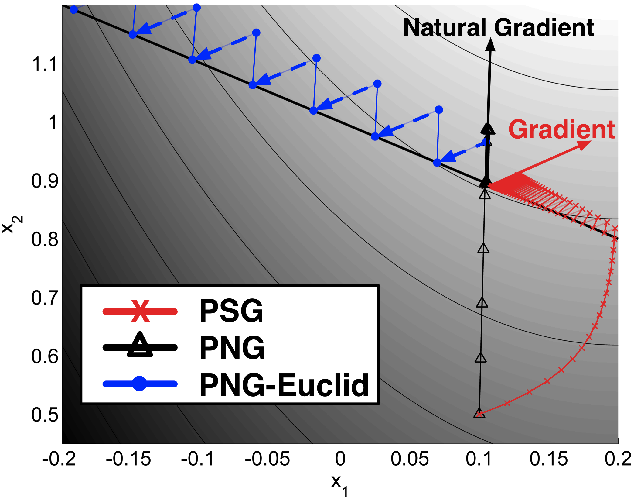
33 Natural Actor-Critic Algorithms
An MDP is a tuple , where is a set of states, is a set of actions, gives the probability density of the system entering state when action is taken in state , is the expected reward, , when action is taken in state , is the initial state distribution, and is a reward discount parameter. A parameterized policy, , is a conditional probability density function— is the probability density of action in state given a vector of policy parameters, .
Let be the discounted-reward objective or the average reward objective function with . Given an MDP, , and a parameterized policy, , the goal is to find policy parameters that maximize one of these objectives. When the action set is continuous, the search for globally optimal policy parameters becomes intractable, so policy search algorithms typically search for locally optimal policy parameters.
Natural actor-critics, first proposed by Kakade [97], are algorithms that estimate and ascend the natural gradient of , using the average Fisher information matrix as the metric tensor:
| (96) |
where is a policy and objective function-dependent distribution over the state set [98].
There are many natural actor-critics, including Natural policy gradient utilizing the Temporal Differences (NTD) algorithm [99], Natural Actor-Critic using LSTD-Q (NAC-LSTD) [100], Episodic Natural Actor-Critic (eNAC) [100], Natural Actor-Critic using Sarsa (NAC-Sarsa) [101], Incremental Natural Actor-Critic (INAC) [102], and Natural-Gradient Actor-Critic with Advantage Parameters (NGAC) [93]. All of them form an estimate, typically denoted , of the natural gradient of . That is, . They then perform the policy parameter update,
34 Projected Natural Actor-Critics
If we are given a closed convex set, , of admissible policy parameters (e.g., the stable region of gains for a PID controller), we may wish to ensure that the policy parameters remain within . The natural actor-critic algorithms described in the previous section do not provide such a guarantee. However, their policy parameter update equations, which are natural gradient ascent updates, can easily be modified to the projected natural gradient ascent update in (91) by projecting the parameters back onto using :
| (97) |
Many of the existing natural policy gradient algorithms, including NAC-LSTD, eNAC, NAC-Sarsa, and INAC, follow biased estimates of the natural policy gradient [103]. For our experiments, we must use an unbiased algorithm since the projection that we propose is compatible with the natural gradient, but not necessarily biased estimates thereof.
NAC-Sarsa and INAC are equivalent biased discounted-reward natural actor-critic algorithms with per-time-step time complexity linear in the number of features. The former was derived by replacing the LSTD-Q component of NAC-LSTD with Sarsa, while the latter is the discounted-reward version of NGAC. Both are similar to NTD, which is a biased average-reward algorithm. The unbiased discounted-reward form of NAC-Sarsa was recently derived [103]. References to NAC-Sarsa hereafter refer to this unbiased variant. In our case studies we use the projected natural actor-critic using Sarsa (PNAC-Sarsa), the projected version of the unbiased NAC-Sarsa algorithm.
Notice that the projection, , as defined in (86), is not merely the Euclidean projection back onto . For example, if is the set of that satisfy , for some fixed matrix and vector , then the projection, , of onto is a quadratic program,
| (98) |
In order to perform this projection, we require an estimate of the average Fisher information matrix, . If the natural actor-critic algorithm does not already include this (like NAC-LSTD and NAC-Sarsa do not), then an estimate can be generated by selecting , where is a positive scalar and is the identity matrix, and then updating the estimate with
| (99) |
where is a stepsize schedule [93]. Notice that we use and subscripts since many time steps of the MDP may pass between updates to the policy parameters.
35 Case Study: Functional Electrical Stimulation
In this case study, we searched for proportional-derivative (PD) gains to control a simulated human arm undergoing FES. We used the Dynamic Arm Simulator 1 (DAS1) [104], a detailed biomechanical simulation of a human arm undergoing functional electrical stimulation. In a previous study, a controller created using DAS1 performed well on an actual human subject undergoing FES, although it required some additional tuning in order to cope with biceps spasticity [85]. This suggests that it is a reasonably accurate model of an ideal arm.
The DAS1 model, depicted in Figure 2a, has state , where and are the desired joint angles, and the desired joint angle velocities are zero. The goal is to, during a two-second episode, move the arm from its random initial state to a randomly chosen stationary target. The arm is controlled by providing a stimulation in the interval to each of six muscles. The reward function used was similar to that of Jagodnik and van den Bogert [85], which punishes joint angle error and high muscle stimulation. We searched for locally optimal PD gains using PNAC-Sarsa where the policy was a PD controller with Gaussian noise added for exploration.
Although DAS1 does not model shoulder dislocation, we added safety constraints by limiting the -norm of certain pairs of gains. The constraints were selected to limit the forces applied to the humerus. These constraints can be expressed in the form , where is a matrix, is a vector, and are the PD gains (policy parameters). We compared the performance of three algorithms:
- 1.
NAC: NAC-Sarsa with no constraints on .
- 2.
PNAC: PNAC-Sarsa using the compatible projection, .
- 3.
PNAC-E: PNAC-Sarsa using the Euclidean projection.
Since we are not promoting the use of one natural actor-critic over another, we did not focus on finely tuning the natural actor-critic nor comparing the learning speeds of different natural actor-critics. Rather, we show the importance of the proper projection by allowing PNAC-Sarsa to run for a million episodes (far longer than required for convergence), after which we plot the mean sum of rewards during the last quarter million episodes. Each algorithm was run ten times, and the results averaged and plotted in Figure 2b. Notice that PNAC performs worse than the unconstrained NAC. This happens because NAC leaves the safe region of policy space during its search, and converges to a dangerous policy—one that reaches the goal quickly and with low total muscle force, but which can cause large, short, spikes in muscle forces surrounding the shoulder, which violates our safety constraints. We suspect that PNAC converges to a near-optimal policy within the region of policy space that we have designated as safe. PNAC-E converges to a policy that is worse than that found by PNAC because it uses an incompatible projection.

36 Case Study: uBot Balancing
In the previous case study, the optimal policy lay outside the designated safe region of policy space (this is common when a single failure is so costly that adding a penalty to the reward function for failure is impractical, since a single failure is unacceptable). We present a second case study in which the optimal policy lies within the designated safe region of policy space, but where an unconstrained search algorithm may enter the unsafe region during its search of policy space (at which point large negative rewards return it to the safe region).
The uBot-5, shown in Figure 20, is an 11-DoF mobile manipulator developed at the University of Massachusetts Amherst [20, 21]. During experiments, it often uses its arms to interact with the world. Here, we consider the problem faced by the controller tasked with keeping the robot balanced during such experiments. To allow for results that are easy to visualize in 2D, we use a PD controller that observes only the current body angle, its time derivative, and the target angle (always vertical). This results in the PD controller having only two gains (tunable policy parameters). We use a crude simulation of the uBot-5 with random upper-body movements, and search for the PD gains that minimize a weighted combination of the energy used and the mean angle error (distance from vertical).
We constructed a set of conservative estimates of the region of stable gains, with which the uBot-5 should never fall, and used PNAC-Sarsa and NAC-Sarsa to search for the optimal gains. Each training episode lasted 20 seconds, but was terminated early (with a large penalty) if the uBot-5 fell over. Figure 20 (middle) shows performance over 100 training episodes. Using NAC-Sarsa, the PD weights often left the conservative estimate of the safe region, which resulted in the uBot-5 falling over. Figure 20 (right) shows one trial where the uBot-5 fell over four times (circled in red). The resulting large punishments cause NAC-Sarsa to quickly return to the safe region of policy space. Using PNAC-Sarsa, the simulated uBot-5 never fell. Both algorithms converge to gains that reside within the safe region of policy space. We selected this example because it shows how, even if the optimal solution resides within the safe region of policy space (unlike the in the previous case study), unconstrained RL algorithms may traverse unsafe regions of policy space during their search.
37 Summary
We presented a class of algorithms, which we call projected natural actor-critics (PNACs). PNACs are the simple modification of existing natural actor-critic algorithms to include a projection of newly computed policy parameters back onto an allowed set of policy parameters (e.g., those of policies that are known to be safe). We argued that a principled projection is the one that results from viewing natural gradient descent, which is an unconstrained algorithm, as a special case of mirror descent, which is a constrained algorithm.
We show that the resulting projection is compatible with the natural gradient and gave a simple empirical example that shows why a compatible projection is important. This example also shows how an incompatible projection can result in natural gradient descent converging to a pessimal solution in situations where a compatible projection results in convergence to an optimal solution. We then applied a PNAC algorithm to a realistic constrained control problem with six-dimensional continuous states and actions. Our results support our claim that the use of an incompatible projection can result in convergence to inferior policies. Finally, we applied PNAC to a simulated robot and showed its substantial benefits over unconstrained natural actor-critic algorithms.
Chapter 6 True Stochastic Gradient Temporal Difference Learning Algorithms
We now turn to the solution of a longstanding puzzle: how to design a “true” gradient method for reinforcement learning? We address long-standing questions in reinforcement learning: (1) Are there any first-order reinforcement learning algorithms that can be viewed as “true” stochastic gradient methods? If there are, what are their objective functions and what are their convergence rates? (2) What is the general framework for avoiding biased sampling (instead of double-sampling, which is a stringent sampling requirement) in reinforcement learning? To this end, we introduce a novel primal-dual splitting framework for reinforcement learning, which shows that the GTD family of algorithms are true stochastic algorithms with respect to the primal-dual formulation of the objective functions such as NEU and MSPBE, which facilitates their convergence rate analysis and regularization. We also propose operator splitting as a unified framework to avoid bias sampling in reinforcement learning. We present an illustrative empirical study on simple canonical problems validating the effectiveness of the proposed algorithms compared with previous approaches.
38 Introduction
First-order temporal difference (TD) learning is a widely used class of techniques in reinforcement learning. Although least-squares based temporal difference approaches, such as LSTD [23], LSPE [24] and LSPI [25] perform well with moderate size problems, first-order temporal difference learning algorithms scale more gracefully to high dimensional problems. The initial class of TD methods was known to converge only when samples are drawn “on-policy”. This motivated the development of the gradient TD (GTD) family of methods [26]. A novel saddle-point framework for sparse regularized GTD was proposed recently [14]. However, there have been several questions regarding the current off-policy TD algorithms. (1) The first is the convergence rate of these algorithms. Although these algorithms are motivated from the gradient of an objective function such as MSPBE and NEU, they are not true stochastic gradient methods with respect to these objective functions, as pointed out in [27], which make the convergence rate and error bound analysis difficult, although asymptotic analysis has been carried out using the ODE approach. (2) The second concern is regarding acceleration. It is believed that TDC performs the best so far of the GTD family of algorithms. One may intuitively ask if there are any gradient TD algorithms that can outperform TDC. (3) The third concern is regarding compactness of the feasible set . The GTD family of algorithms all assume that the feasible set is unbounded, and if the feasible set is compact, there is no theoretical analysis and convergence guarantee. (4) The fourth question is on regularization: although the saddle point framework proposed in [14] provides an online regularization framework for the GTD family of algorithms, termed as RO-TD, it is based on the inverse problem formulation and is thus not quite explicit. One further question is whether there is a more straightforward algorithm, e.g, the regularization is directly based on the MSPBE and NEU objective functions.
Biased sampling is a well-known problem in reinforcement learning. Biased sampling is caused by the stochasticity of the policy wherein there are multiple possible successor states from the current state where the agent is. If it is a deterministic policy, then there will be no biased sampling problem. Biased sampling is often caused by the product of the TD errors, or the product of TD error and the gradient of TD error w.r.t the model parameter . There are two ways to avoid the biased sampling problem, which can be categorized into double sampling methods and two-time-scale stochastic approximation methods.
In this paper, we propose a novel approach to TD algorithm design in reinforcement learning, based on introducing the proximal splitting framework [28]. We show that the GTD family of algorithms are true stochastic gradient descent (SGD) methods, thus making their convergence rate analysis available. New accelerated off-policy algorithms are proposed and their comparative study with RO-TD is carried out to show the effectiveness of the proposed algorithms. We also show that primal-dual splitting is a unified first-order optimization framework to solve the biased sampling problem.
Here is a roadmap to the rest of the chapter. Section 2 reviews reinforcement learning and the basics of proximal splitting formulations and algorithms. Section 3 introduces a novel problem formulation which we investigate in this paper. Section 4 proposes a series of new algorithms, demonstrates the connection with the GTD algorithm family, and also presents accelerated algorithms. Section 5 presents theoretical analysis of the algorithms. Finally, empirical results are presented in Section 6 which validate the effectiveness of the proposed algorithmic framework. Abbreviated technical proofs of the main theoretical results are provided in a supplementary appendix.
39 Background
39.1 Markov Decision Process and Reinforcement Learning
In linear value function approximation, a value function is assumed to lie in the linear span of a basis function matrix of dimension , where is the number of linear independent features. Hence, . For the -th sample, (the -th row of ), (the -th row of ) are the feature vectors corresponding to , respectively. is the weight vector for -th sample in first-order TD learning methods, and is the temporal difference error. TD learning uses the following update rule , where is the stepsize. However, TD is only guaranteed to converge in the on-policy setting, although in many off-policy situations, it still has satisfactory performance [105]. To this end, Sutton et al. proposed a family of off-policy convergent algorithms including GTD, GTD2 and TD with gradient correction (TDC). GTD is a two-time-scale stochastic approximation approach which aims to minimize the norm of the expected TD update (NEU), which is defined as
| (100) |
TDC [26] aims to minimize the mean-square projected Bellman error (MSPBE) with a similar two-time-scale technique, which is defined as
| (101) |
where is a diagonal matrix whose entries are given by a positive probability distribution over states.
40 Problem Formulation
Biased sampling is a well-known problem in reinforcement learning. Biased sampling is caused by or , where is the feature vector for state in sample . Due to the stochastic nature of the policy, there may be many w.r.t the same , thus or cannot be consistently estimated via a single sample. This problem hinders the objective functions to be solved via stochastic gradient descent (SGD) algorithms. As pointed out in [27], although many algorithms are motivated by well-defined convex objective functions such as MSPBE and NEU, due to the biased sampling problem, the unbiased stochastic gradient is impossible to obtain, and thus the algorithms are not true SGD methods w.r.t. these objective functions. The biased sampling is often caused by the product of the TD errors, or the product of TD error and the derivative of TD error w.r.t. the parameter . There are two ways to avoid the biased sampling problem, which can be categorized into double sampling methods and stochastic approximation methods. Double sampling, which samples both and and thus requires computing and , is possible in batch reinforcement learning, but is usually impractical in online reinforcement learning. The other approach is stochastic approximation, which introduces a new variable to estimate the part containing , thus avoiding the product of and . Consider, for example, the NEU objective function in Section (100). Taking the gradient w.r.t. , we have
| (102) |
If the gradient can be written as a single expectation value, then it is straightforward to use a stochastic gradient method, however, here we have a product of two expectations, and due to the correlation between and , the sampled product is not an unbiased estimate of the gradient. In other words, and can be directly sampled, yet can not be directly sampled. To tackle this, the GTD algorithm uses the two-time-scale stochastic approximation method by introducing an auxiliary variable , and thus the method is not a true stochastic gradient method w.r.t. any more. This auxiliary variable technique is also used in [56].
The other problem for first-order reinforcement learning algorithms is that it is difficult to define the objective functions, which is also caused by the biased sampling problem. As pointed out in [27], although the GTD family of algorithms are derived from the gradient w.r.t. the objective functions such as MSPBE and NEU, because of the biased-sampling problem, these algorithms cannot be formulated directly as SGD methods w.r.t. these objective functions.
In sum, due to biased sampling, the RL objective functions cannot be solved via a stochastic gradient method, and it is also difficult to find objective functions of existing first-order reinforcement learning algorithms. Thus, there remains a large gap between first-order reinforcement learning algorithms and stochastic optimization, which we now show how to bridge.
41 Algorithm Design
In what follows, we build on the operator splitting methods introduced in Section 12.3, which should be reviewed before reading the section below.
41.1 NEU Objective Function
41.2 MSPBE Objective Function
Based on the definition of MSPBE in Section (100), we can reformulate MSPBE as
| (105) |
The gradient of MSPBE is correspondingly computed as
| (106) |
As opposed to computing the NEU gradient, computing Equation (106) involves computing the inverse matrix , which imposes extra difficulty. To this end, we propose another primal-dual splitting formulation with weighted Euclidean norm as follows,
| (107) |
where , and the dual variable is denoted as to differentiate it from used for the NEU objective function. Then we have
| (108) |
Note that the nonlinear convex , and thus the Legendre transform is . We can see that by using the primal-dual splitting formulation, computing the inverse matrix is avoided. Thus the update rule is as follows:
| (109) |
Note that if and , then we will have the GTD2 algorithm proposed in [26]. It is also worth noting that the TDC algorithm seems not to have an explicit proximal splitting representation, since it incorporates into the update of , a quasi-stationary condition which is commonly used in two-time-scale stochastic approximation approaches. An intuitive answer to the advantage of TDC over GTD2 is that the TDC update of can be considered as incorporating the prior knowledge into the update rule: for a stationary , if the optimal (termed as ) has a closed-form solution or is easy to compute, then incorporating this into the update rule tends to accelerate the algorithm’s convergence performance. For the GTD2 update in Equation (109), note that there is a sum of two terms where appears: which are . Replacing in the first term with , we have the update rule as follows
| (110) |
Note that if and , then we will have TDC algorithm proposed in [26]. Note that this technique does not have the same convergence guarantee as the original objective function. For example, if we use a similar trick on the GTD update with the optimal (termed as ) where , then we can have
| (111) |
which is the update rule of residual gradient [107], and is proven not to converge to NEU any more.99 9 It converges to mean-square TD error (MSTDE), as proven in [75].
42 Accelerated Gradient Temporal Difference Learning Algorithms
In this section we will discuss the acceleration of GTD2 and TDC. The acceleration of GTD is not discussed due to space consideration, which is similar to GTD2. A comprehensive overview of the convergence rate of different approaches to stochastic saddle-point problems is given in [108]. In this section we present accelerated algorithms based on the Stochastic Mirror-Prox (SMP) Algorithm [47, 109]. Algorithm 11, termed as GTD2-MP, is accelerated GTD2 with extragradient. Algorithm 12, termed as TDC-MP, is accelerated TDC with extragradient.
Let be some fixed policy of an MDP , be some fixed basis.
- 1.
- 2.
- 3.
- 1.
- 2.
- 3.
43 Theoretical Analysis
In this section, we discuss the convergence rate and error bound of GTD, GTD2 and GTD2-MP.
43.1 Convergence Rate
Proposition 1 The convergence rates of the GTD/GTD2 algorithms with primal average are , where , for GTD, and for GTD2, , is defined in the Appendix due to space limitations.
Now we consider the convergence rate of GTD2-MP.
Proposition 2 The convergence rate of the GTD2-MP algorithm is .
See supplementary materials for an abbreviated proof. Remark: The above propositions imply that when the noise level is low, the GTD2-MP algorithm is able to converge at the rate of , whereas the convergence rate of GTD2 is . However, when the noise level is high, both algorithms’ convergence rates reduce to .
43.2 Value Approximation Error Bound
Proposition 3: For GTD/GTD2, the prediction error of is bounded by ; For GTD2-MP, it is bounded by , where .
Proof: see Appendix.
43.3 Related Work
Here we will discuss previous related work. To the best of our knowledge, the closest related work is the RO-TD algorithm, which first introduced the convex-concave saddle-point framework to regularize the TDC family of algorithms. 1010 10 Although only regularized TDC was proposed in [14], the algorithm can be easily extended to regularized GTD and GTD2. The major difference is that RO-TD is motivated by the linear inverse problem formulation of TDC algorithm and uses its dual norm representation as the objective function, which does not explore the auxiliary variable . In contrast, by introducing the operator splitting framework, we demonstrate that the GTD family of algorithms can be nicely explained as a “true” SGD approach, where the auxiliary variable has a nice explanation.
Another interesting question is whether ADMM is suitable for the operator splitting algorithm here. Let’s take NEU for example. The ADMM formulation is as follows, where we assume for simplicity, and other scenarios can be derived similarly,
| (112) |
The update rule is as follows, where is the stepsize
| (113) |
At first glance the operator of and seem to be split, however, if we compute the closed-form update rule of , we can see that the update of includes , which involves both biased-sampling and computing the inverse matrix, thus regular ADMM does not seem to be practical for this first-order reinforcement learning setting. However, using the pre-conditioning technique introduced in [110], ADMM can be reduced to the primal-dual splitting method as pointed out in [58].
44 Experimental Study
44.1 Off-Policy Convergence: Baird Example
The Baird example is a well-known example where TD diverges and TDC converges. The stepsizes are set to be constants where as shown in Figure 21. From Figure 21, we can see that GTD2-MP and TDC-MP have a significant advantage over the GTD2 and TDC algorithms wherein both the MSPBE and the variance are substantially reduced.
44.2 Regularization Solution Path: Two-State Example
Now we consider the two-state MDP in [111]. The transition matrix and reward vector are and , and a one-feature basis . The objective function are , where is and . The objective functions are termed as -NEU and -MSPBE for short. In Figure 22, both -NEU and -MSPBE have well-defined solution paths w.r.t , whereas Lasso-TD may have multiple solutions if the -matrix condition is not satisfied [62].
44.3 On-Policy Performance: -State Random MDP
In this experiment we compare the on-policy performance of the four algorithms. We use the random generated MDP with states and actions in [112]. Each state is represented by a feature vector with features, where features are generated by sampling from a uniform distribution the -th feature is a constant. The stepsizes are set to be constants where as shown in Figure 23. The parameters of each algorithm are chosen via comparative studies similar to [112]. The result is shown in Figure 23. The results for each algorithm are averaged on runs, and the parameters of each algorithm are chosen via experiments. TDC shows high variance and chattering effect of MSPBE curve on this domain. Compared with GTD2, GTD2-M1P is able to reduce the MSPBE significantly. Compared with TDC, TDC-MP not only reduces the MSPBE, but also the variance and the ”chattering” effect.

45 Summary
This chapter shows that the GTD/GTD2 algorithms are true stochastic gradient methods w.r.t. the primal-dual formulation of their corresponding objective functions, which enables their convergence rate analysis and regularization. Second, it proposes operator splitting as a broad framework to solve the biased-sampling problem in reinforcement learning. Based on the unified primal-dual splitting framework, it also proposes accelerated algorithms with both rigorous theoretical analysis and illustrates their improved performance w.r.t. previous methods. Future research is ongoing to explore other operator splitting techniques beyond primal-dual splitting as well as incorporating random projections [113], and investigating kernelized algorithms [114, 115]. Finally, exploring the convergence rate of the TDC algorithm is also important and interesting.
Chapter 7 Variational Inequalities: The Emerging Frontier of Machine Learning
This paper describes a new framework for reinforcement learning based on primal dual spaces connected by a Legendre transform. The ensuing theory yields surprising and beautiful solutions to several important questions that have remained unresolved: (i) how to design reliable, convergent, and stable reinforcement learning algorithms (ii) how to guarantee that reinforcement learning satisfies pre-specified “safety” guarantees, and remains in a stable region of the parameter space (iv) how to design “off-policy” TD-learning algorithms in a reliable and stable manner, and finally, (iii) how to integrate the study of reinforcement learning into the rich theory of stochastic optimization. In this paper, we gave detailed answers to all these questions using the powerful framework of proximal operators. The single most important idea that emerges is the use of primal dual spaces connected through the use of a Legendre transform. This allows temporal-difference updates to occur in dual spaces, allowing a variety of important technical advantages. The Legendre transform, as we show, elegantly generalizes past algorithms for solving reinforcement learning problems, such as natural gradient methods, which we show relate closely to the previously unconnected framework of mirror descent methods. Equally importantly, proximal operator theory enables the systematic development of operator splitting methods that show how to safely and reliably decompose complex products of gradients that occur in recent variants of gradient-based temporal-difference learning. This key technical contribution makes it possible to finally show to design “true” stochastic gradient methods for reinforcement learning. Finally, Legendre transforms enable a variety of other benefits, including modeling sparsity and domain geometry. Our work builds extensively on recent work on the convergence of saddle-point algorithms, and on the theory of monotone operators in Hilbert spaces, both in optimization and for variational inequalities. The latter represents possibly the most exciting future research direction, and we give a more detailed description of this ongoing research thrust.
46 Variational Inequalities
Our discussion above has repeatedly revolved around the fringes of variational inequality theory. Methods like extragradient [8] and the mirror-prox algorithm were originally proposed to solve variational inequalities and related saddle point problems. We are currently engaged in redeveloping the proposed ideas more fully within the fabric of variational inequality (VI). Accordingly, we briefly describe the framework of VIs, and give the reader a brief tour of this fascinating extension of the basic underlying framework of optimization. We lack the space to do a thorough review. That is the topic of another monograph to be published at a later date, and several papers on this topic are already under way.
At the dawn of a new millennium, the Internet dominates our economic, intellectual and social lives. The concept of equilibrium plays a key role in understanding not only the Internet, but also other networked systems, such as human migration [116], evolutionary dynamics and the spread of infectious diseases [117], and social networks [118]. Equilibria are also a central idea in game theory [119, 120], economics [121], operations research [29], and many related areas. We are currently exploring two powerful mathematical tools for the study of equilibria – variational inequalities (VIs) and projected dynamical systems (PDS) [12, 122] – in developing a new machine learning framework for solving equilibrium problems in a rich and diverse range of practical applications. As Figure 24 illustrates, finite-dimensional VIs provide a mathematical framework that unifies many disparate equilibrium problems of significant importance, including (convex) optimization, equilibrium problems in economics, game theory and networks, linear and nonlinear complementarity problems, and solutions of systems of nonlinear equations.

Variational inequalities (VIs), in the infinite-dimensional setting, were originally proposed by Hartman and Stampacchia [10] in the mid-1960s in the context of solving partial differential equations in mechanics. Finite-dimensional VIs rose in popularity in the 1980s partly as a result of work by Dafermos [11]. who showed that the traffic network equilibrium problem could be formulated as a finite-dimensional VI. This advance inspired much follow-on research, showing that a variety of equilibrium problems in economics, game theory, sequential decision-making etc. could also be formulated as finite-dimensional VIs – the books by Nagurney [12] and Facchinei and Pang [13] provide a detailed introduction to the theory and applications of finite-dimensional VIs. Projected dynamical systems (PDS) [122] are a class of ordinary differential equations (ODEs) with a discontinuous right-hand side. Associated with every finite-dimensional VI is a PDS, whose stationary points are the solutions of the VI. While VIs provide a static analysis of equilibria, PDS enable a microscopic examination of the dynamic processes that lead to or away from stable equilibria. . There has been longstanding interest in AI in the development of gradient-based learning algorithms for finding Nash equilibria in multiplayer games, e.g. [123, 119, 124]. A gradient method for finding Nash equilibria can be formalized by a set of ordinary differential equations, whose phase space portrait solution reveals the dynamical process of convergence to an equilibrium point, or lack thereof. A key complication in this type of analysis is that the classical dynamical systems approach does not allow incorporating constraints on values of variables, which are omnipresent in equilibria problems, not only in games, but also in many other applications in economics, network flow, traffic modeling etc. In contrast, the right-hand side of a PDS is a discontinuous projection operator that allows enabling constraints to be modeled.
One of the original algorithms for solving finite-dimensional VIs is the extragradient method proposed by Korpelevich [125]. It has been applied to structured prediction models in machine learning by Taskar et al. [126]. Bruckner et al. [127] use a modified extragradient method for solving the spam filtering problem modeled as a prediction game. We are developing a new family of extragradient-like methods based on well-known numerical methods for solving ordinary differential equations, specifically the Runge Kutta method [128]. In optimization, the extragradient algorithm was generalized to the non-Euclidean case by combining it with the mirror-descent method [5], resulting in the so-called “mirrror-prox” algorithm [129, 130]. We have extended the mirror-prox method by combining it with Runge-Kutta methods for solving high-dimensional VI problems over the simplex and other spaces. We show the enhanced performance of Runge-Kutta extragradient methods on a range of benchmark variational inequalities drawn from standard problems in the optimization literature.
46.1 Definition
The formal definition of a VI as follows:1111 11 Variational problems can be defined more abstractly in Hilbert spaces. We confine our discussion to -dimensional Euclidean spaces.
Definition 46.1.
The finite-dimensional variational inequality problem VI(F,K) involves finding a vector such that
where is a given continuous function and is a given closed convex set, and is the standard inner product in .
Figure 25 provides a geometric interpretation of a variational inequality. 1212 12 In Figure 25, the normal cone at the vector of a convex set is defined as . The following general result characterizes when solutions to VIs exist:
Theorem 46.2.
Suppose is compact, and that is continuous. Then, there exists a solution to VI().
As Figure 25 shows, is a solution to if and only if the angle between the vectors and , for any vector , is less than or equal to . To build up some intuition, the reduction of a few well-known problems to a VI is now provided.
Theorem 46.3.
Let be a solution to the optimization problem of minimizing a continuously differentiable function , subject to , where is a closed and convex set. Then, is a solution to , such that .
Proof: Define . Since is minimized at , it follows that , that is solves the VI.
Theorem 46.4.
If is a convex function, and is the solution of , then minimizes .
Proof: Since is convex, it follows that any tangent lies below the function, that is . But, since solves the VI, it follows that is a lower bound on the value of everywhere, or that minimizes .
A rich class of problems called complementarity problems (CPs) also can be reduced to solving a VI. When the feasible set is a cone, meaning that if , then , then the VI becomes a CP.
Definition 46.5.
Given a cone , and a mapping , the complementarity problem CP(F,K) is to find an such that , the dual cone to , and . 1313 13 Given a cone , the dual cone is defined as .
A number of special cases of CPs are important. The nonlinear complementarity problem (NCP) is to find (the non-negative orthant) such that and . The solution to an NCP and the corresponding are the same, showing that NCPs reduce to VIs. In an NCP, whenever the mapping function is affine, that is , where is an matrix, then the corresponding NCP is called a linear complementarity problem (LCP) [131]. Recent work on learning sparse models using regularization has exploited the fact that the standard LASSO objective [132] of penalized regression can be reduced to solving an LCP [133]. This reduction to LCP has been used in recent work on sparse value function approximation as well in a method called LCP-TD [134]. A final crucial property of VIs is that they can be formulated as finding fixed points.
Theorem 46.6.
The vector is the solution of VI(F,K) if and only if, for any , is also a fixed point of the map , where is the projector onto convex set .
In terms of the geometric picture of a VI illustrated in Figure 25. this property means that the solution of a VI occurs at a vector where the vector field induced by on is normal to the boundary of and directed inwards, so that the projection of is the vector itself. This property forms the basis for the projection class of methods that solve for the fixed point.
46.2 Equilibrium Problems in Game Theory
The VI framework provides a mathematically elegant approach to model equilibrium problems in game theory [119, 120]. A Nash game consists of players, where player chooses a strategy belonging to a closed convex set . After executing the joint action, each player is penalized (or rewarded) by the amount , where is a continuously differentiable function. A set of strategies is said to be in equilibrium if no player can reduce the incurred penalty (or increase the incurred reward) by unilaterally deviating from the chosen strategy. If each is convex on the set , then the set of strategies is in equilibrium if and only if . In other words, needs to be a solution of the VI , where . Nash games are closely related to saddle point problems [129, 130, 135]. where we are given a function , and the objective is to find a solution such that
Here, is convex in for each fixed , and concave in for each fixed . Many equilibria problems in economics can be modeled using VIs [12].
47 Algorithms for Variational Inequalities
We briefly describe two algorithms for solving variational inequalities below: the projection method and the extragradient method. We conclude with a brief discussion of how these relate to reinforcement learning.
47.1 Projection-Based Algorithms for VIs
The basic projection-based method (Algorithm 1) for solving VIs is based on Theorem 46.6 introduced earlier.
INPUT: Given VI(F,K), and a symmetric positive definite matrix .
Here, is the projector onto convex set with respect to the natural norm induced by , where . It can be shown that the basic projection algorithm solves any for which the mapping is strongly monotone 1414 14 A mapping is strongly monotone if . and Lipschitz.1515 15 A mapping is Lipschitz if . A simple strategy is to set , where , and is the Lipschitz smoothness constant, and is the strong monotonicity constant. The basic projection-based algorithm has two critical limitations: it requires that the mapping be strongly monotone. If, for example, is the gradient map of a continuously differentiable function, strong monotonicity implies the function must be strongly convex. Second, setting the parameter requires knowing the Lipschitz smoothness and the strong monotonicity parameter . The extragradient method of Korpolevich [125] addresses some of these concerns, and is defined as Algorithm 2 below.
INPUT: Given VI(F,K), and a scalar .
Figure 26 shows a simple example where Algorithm 1 fails to converge, but Algorithm 2 does. If the initial point is chosen to be on the boundary of , using Algorithm 1, it stays on it and fails to converge to the solution of this VI (which is at the origin). If is chosen to be in the interior of , Algorithm 1 will move towards the boundary. In contrast, using Algorithm 2, the solution can be found for any starting point. The extragradient algoriithm derives its name from the property that it requires an “extra gradient” step (step 4 in Algorithm 2), unlike the basic projection algorithm given earlier as Algorithm 1. The principal advantage of the extragradient method is that it can be shown to converge under a considerably weaker condition on the mapping , which now has to be merely monotonic: . The earlier Lipschitz condition is still necessary for convergence.
The extragradient algorithm has been the topic of much attention in optimization since it was proposed, e.g., see [137, 138, 139, 140, 141, 142]. Khobotov [138] proved that the extragradient method converges under the weaker requirement of pseudo-monotone mappings, 1616 16 A mapping is pseudo-monotone if . when the learning rate is automatically adjusted based on a local measure of the Lipschitz constant. Iusem [137] proposed a variant whereby the current iterate was projected onto a hyperplane separating the current iterate from the final solution, and subsequently projected from the hyperplane onto the feasible set. Solodov and Svaiter [142] proposed another hyperplane method, whereby the current iterate is projected onto the intersection of the hyperplane and the feasible set. Finally, the extragradient method was generalized to the non-Euclidean case by combining it with the mirror-descent method [5], resulting in the so-called “mirrror-prox” algorithm [129].
47.2 Variational Inequaities and Reinforcement Learning
Variational inequalities also provide a useful framework for reinforcement learning [32, 1]. In this case, it can be shown that the mapping for the VI defined by reinforcement learning is affine and represents a (linear) complementarity problem. For this case, a number of special properties can be exploited in designing a faster more scalable class of algorithms. Recall from Theorem 46.6 that each VI(F,K) corresponds to solving a particular fixed point problem , which led to the projection algorithm (Algorithm 1). Generalizing this, consider solving for the fixed point of a projected equation [143, 144] for a functional mapping , where is the projector onto a low-dimensional convex subspace w.r.t. some positive definite matrix , so that
| (114) |
Here. is an matrix where , and the goal is to make the computation depend on , not . Note that if and only if
Following [143], note that this is a variational inequality of the form if we identify , and in the lower-dimensional space, . Hence, the projection algorithm takes on the form:
It is shown in [143] that if is a contraction mapping, then is strongly monotone. Hence, the above projection algorithm will converge to the solution of the VI for any given starting point . Now, the only problem is how to ensure the computation depends only on the size of the projected lower-dimensional space (i.e., , not ). To achieve this, let us assume that the mapping is affine, and that the constraint region is polyhedral. In this case, we can use the following identities:
and the projection algorithm for this affine case can be written as:
One way to solve this iteratively is to compute a progressively more accurate approximation and by sampling from the rows and columns of the matrix and vector , as follows:
where the row sampling generates the indices and the column sampling generates the transitions in such a way that the relative frequency of row index matches the diagonal element of the positive definite matrix . Given and , the solution can be found by , or by using an incremental method. Computation now only depends on the dimension of the lower-dimensional space, not on the original high-dimensional space. Gordon [144] proposes an alternative approach separating the projection of the current iterate on the low-dimensional subspace spanned by from its projection onto the feasible set. Both of these approaches [143, 144] have been only studied with the simple projection method (Algorithm 1), and can be generalized to a more powerful class of VI methods that we are currently developing.
Acknowledgements
We like to acknowledge the useful feedback of past and present members of the Autonomous Learning Laboratory at the University of Massachusetts, Amherst. Principal funding for this research was provided by the National Science Foundation under the grant NSF IIS-1216467. Past work by the first author has been funded by NSF grants IIS-0534999 and IIS-0803288.
Chapter 8 Appendix: Technical Proofs
48 Convergence Analysis of Saddle Point Temporal Difference Learning
Proof of Proposition 1
We give a descriptive proof here. We first present the monotone operator corresponding to the bilinear saddle-point problem and then extend it to stochastic approximation case with certain restrictive assumptions, and use the result in [47].
The monotone operator with saddle-point problem is a point-to-set operator
Where is the subgradient of over and is the subgradient of over . For the bilinear problem in Equation (54), the corresponding is
| (115) |
Now we verify that the problem (65) can be reduced to a standard bilinear minimax problem. To prove this we only need to prove in our RL problem is indeed a closed compact convex set. This is easy to verify as we can simply define where is large enough. In fact, the sparse regularization helps stay within this ball. Now we extend to the stochastic approximation case wherein the objective function is given by the stochastic oracle, and in our case, it is , where are defined in Equation (62), with Assumption 3 and further assuming that the noise for -th sample is i.i.d noise, then with the result in [109], we can prove that the RO-TD algorithm converges to the global minimizer of
Then we prove the error level of approximate saddle-point defined in (71) is . With the subgradient boundedness assumption and using the result in Proposition 1 in [78], this can be proved.
49 Convergence Analysis of True Gradient Temporal Difference Learning
Assumption 1 (MDP): The underlying Markov Reward Process (MRP) is finite and mixing, with stationary distribution . The training sequence is an i.i.d sequence.
Assumption 2 (Basis Function): The inverses
and exist.
This implies that is a full column rank matrix. Also, assume
the features have uniformly bounded second
moments, and .
Next we present the assumptions for the stochastic saddle point problem
formulation, which are similar to [108, 109].
Assumption 3 (Compactness): Assume for the primal-dual loss function,
| (116) |
the sets are closed compact sets.
Assumption 4 (): We assume that is a smooth convex function with Lipschitz continuous gradient, i.e., such that
| (117) |
Assumption 5 (): is a linear mapping which can be extended to Lipschitz continuous vector-valued mapping defined on a closed convex cone . Assuming to be -convex, i.e.,
where means that .
Assumption 6 (Stochastic Gradient): In the stochastic saddle point problem, we assume that there exists a stochastic oracle that is able to provide unbiased estimation with bounded variance such that
| (118) |
| (119) |
| (120) |
where , and are non-negative constants. We further define
| (121) |
49.1 Convergence Rate
Here we discuss the convergence rate of the proposed algorithms. First let us review the nonlinear primal form
| (122) |
The corresponding primal-dual formulation [57, 28, 58] of Equation (122) is Equation (40). Thus we have the general update rule as
| (123) |
Lemma 1 (Optimal Convergence Rate): The optimal convergence rate of 40 is .
Proof: Equation (122) can be easily converted to the following primal-dual formulation
| (124) |
Using the bounds proved in [145, 109, 108], the optimal convergence rate of stochastic saddle-point problem is .
The GTD/GTD2 algorithms can be considered as using Polyak’s algorithm without the primal average step. Hence, by adding the primal average step, GTD/GTD2 algorithms will become standard Polyak’s algorithms [146], and thus the convergence rates are according to [49]. So we have the following propositions.
Proposition 1 The convergence rates of GTD/GTD2 algorithms with primal average are , where , for GTD, and for GTD2, .
Now we consider the acceleration using the SMP algorithm, which incorporates the extragradient term. According to [109] which extends the SMP algorithm to solving saddle-point problems and variational inequality problems, the convergence rate is accelerated to . Consequently,
Proposition 2 The convergence rate of the GTD2-MP algorithm is .
49.2 Value Approximation Error Bound
One key question is how to give the error bound of given that of . Here we use the result in [111], which is similar to the one in [147].
Use the equality and , where the first equality is the Bellman equation, and the second is that lies within the spanning space of .
Proposition 3: For GTD/GTD2, the prediction error of is bounded by ; For GTD2-MP, it is bounded by , where .
Proof:
From Lemma 2, we have
| (128) |
Using the results in Proposition 1 and Proposition 2, we have for GTD and GTD2,
| (129) |
For GTD2-MP,
| (130) |
If we further assume a rich expressive hypothesis space , i.e., , , then for GTD and GTD2, we have
| (131) |
For GTD2-MP, we have
| (132) |
References
- [1] R. Sutton and A. G. Barto. Reinforcement Learning: An Introduction. MIT Press, 1998.
- [2] Richard S. Sutton, Hamid Reza Maei, Doina Precup, Shalabh Bhatnagar, David Silver, Csaba Szepesvári, and Eric Wiewiora. Fast gradient-descent methods for temporal-difference learning with linear function approximation. In In Proceedings of the 26th International Conference on Machine Learning, 2009a.
- [3] S. Boyd and L. Vandenberghe. Convex Optimization. Cambridge University Press, 2004.
- [4] L. Bregman. The relaxation method of finding the common point of convex sets and its application to the solution of problems in convex programming. USSR Computational Mathematics and Mathematical Physics, 7:200–217, 1967.
- [5] A. Nemirovksi and D. Yudin. Problem Complexity and Method Efficiency in Optimization. John Wiley Press, 1983.
- [6] A. Beck and M. Teboulle. Mirror descent and nonlinear projected subgradient methods for convex optimization. Operations Research Letters, Jan 2003a. URL http://www.sciencedirect.com/science/article/pii/S0167637702002316.
- [7] A. Nemirovski. Prox-method with rate of convergence O(1/t) for variational inequalities with Lipschitz continuous monotone operators and smooth convex-concave saddle point problems. SIAM Journal on Optimization, 15(1):229–251, 2005.
- [8] G. M. Korpelevich. The extragradient method for finding saddle points and other problems. 1976.
- [9] S. Bubeck. Theory of convex optimization for machine learning. Unpublished Manuscript.
- [10] P. Hartman and G. Stampacchia. On some nonlinear elliptic differential functional equations. Acta Mathematica, 115:271–310, 1966.
- [11] S. Dafermos. Traffic equilibria and variational inequalities. Transportation Science, 14:42–54, 1980.
- [12] A. Nagurney. Network Economics: A Variational Inequality Approach. Kluwer Academic Press, 1999.
- [13] F. Facchinei and Pang J. Finite-Dimensional Variational Inequalities and Complimentarity Problems. Springer, 2003.
- [14] B. Liu, S. Mahadevan, and J. Liu. Regularized off-policy TD-learning. In Advances in Neural Information Processing Systems 25, pages 845–853, 2012a.
- [15] A. Ben-Tal, T. Margalit, and A. Nemirovski. The ordered subsets mirror descent optimization method with applications to tomography. SIAM Journal of Optimization, Jan 2001. URL http://132.68.160.12/Labs/Opt/opt/Pap/SIAM_ppr_fin.pdf.
- [16] Claudio Gentile. The robustness of the p-norm algorithms. Mach. Learn., 53:265–299, December 2003a. ISSN 0885-6125. 10.1023/A:1026319107706. URL http://dl.acm.org/citation.cfm?id=948445.948447.
- [17] P. Combetes and J.C. Pesquel. Proximal splitting methods in signal processing. In Fixed-Point Algorithms for Inverse Problems in Science and Engineering. Springer, 2011.
- [18] J. Douglas and H. Rachford. On the numerical solution of heat conduction problems in two and three space variables. Transactions of the American Mathematical Society, 82:421–439, 1956.
- [19] S. Boyd, N. Parikh, E. Chu, B. Peleato, and J. Eckstein. Distributed optimization and statistical learning via the alternating direction method of multipliers. Foundations and Trends in Machine Learning, 3(1):1–122, 2010.
- [20] P. Deegan. Whole-Body Strategies for Mobility and Manipulation. PhD thesis, University of Massachusetts Amherst, 2010.
- [21] S. R. Kuindersma, E. Hannigan, D. Ruiken, and R. A. Grupen. Dexterous mobility with the uBot-5 mobile manipulator. In Proceedings of the 14th International Conference on Advanced Robotics, 2009.
- [22] S. Amari and S. Douglas. Why natural gradient? In Proceedings of the 1998 IEEE International Conference on Acoustics, Speech, and Signal Processing, volume 2, pages 1213–1216, 1998.
- [23] S. Bradtke and A. Barto. Linear least-squares algorithms for temporal difference learning. Machine Learning, 22:33–57, 1996.
- [24] A. Nedic and D. Bertsekas. Least-squares policy evaluation algorithms with linear function approximation. Discrete Event Systems Journal, 13, 2003.
- [25] M. Lagoudakis and R. Parr. Least-squares policy iteration. Journal of Machine Learning Research, 4:1107–1149, 2003.
- [26] R.S. Sutton, H.R. Maei, D. Precup, S. Bhatnagar, D. Silver, C. Szepesvári, and E. Wiewiora. Fast gradient-descent methods for temporal-difference learning with linear function approximation. In International Conference on Machine Learning, pages 993–1000, 2009b.
- [27] C. Szepesvári. Algorithms for reinforcement learning. Synthesis Lectures on Artificial Intelligence and Machine Learning, 4(1):1–103, 2010.
- [28] P. L Combettes and J. C Pesquet. Proximal splitting methods in signal processing. In Fixed-point algorithms for inverse problems in science and engineering, pages 185–212. 2011.
- [29] M. L. Puterman. Markov Decision Processes. Wiley Interscience, New York, USA, 1994.
- [30] R. S. Sutton. Learning to predict by the methods of temporal differences. Machine Learning, 3:9–44, 1988. URL citeseer.ist.psu.edu/sutton88learning.html.
- [31] C. Watkins. Learning from Delayed Rewards. PhD thesis, King’s College, Cambridge, England, 1989.
- [32] D. Bertsekas and J. Tsitsiklis. Neuro-Dynamic Programming. Athena Scientific, Belmont, Massachusetts, 1996.
- [33] S. Mahadevan. Learning representation and control in Markov Decision Processes: new frontiers. Foundations and Trends in Machine Learning, 1(4):403–565, 2009.
- [34] G. Lan. An optimal method for stochastic composite optimization. Mathematical Programming, 133(1-2):365–397, 2012.
- [35] A. Beck and M. Teboulle. Mirror descent and nonlinear projected subgradient methods for convex optimization. Operations Research Letters, 31:167–175, 2003b.
- [36] C. Gentile. The robustness of the p-norm algorithms. Machine Learning, 53(3):265–299, 2003b.
- [37] S. Shalev-Shwartz and A. Tewari. Stochastic methods for l1 regularized loss minimization. Journal of Machine Learning Research, pages 1865–1892, June 2011.
- [38] L. Xiao. Dual averaging methods for regularized stochastic learning and online optimization. The Journal of Machine Learning Research, 11:2543–2596, 2010.
- [39] J. Duchi, S. Shalev-Shwartz, Y. Singer, and A. Tewari. Composite objective mirror descent. In COLT, pages 14–26, 2010a.
- [40] J. Gao, T. Xu, L. Xiao, and X. He. A voted regularized dual averaging method for large-scale discriminative training in natural language processing. Technical report, Microsoft Research, 2013.
- [41] H. B. McMahan. Follow-the-regularized-leader and mirror descent: Equivalence theorems and l1 regularization. In International Conference on Artificial Intelligence and Statistics, pages 525–533, 2011.
- [42] J. Langford, L. Li, and T. Zhang. Sparse online learning via truncated gradient. The Journal of Machine Learning Research, 10:777–801, 2009.
- [43] S. Shalev-Shwartz and A. Tewari. Stochastic methods for l1 regularized loss minimization. In Proceedings of the 26th Annual International Conference on Machine Learning, pages 929–936, 2009.
- [44] S. Lee and S.J. Wright. Manifold identification in dual averaging for regularized stochastic online learning. The Journal of Machine Learning Research, pages 1705–1744, 2012.
- [45] P. Tseng. On accelerated proximal gradient methods for convex-concave optimization. submitted to SIAM Journal on Optimization, 2008.
- [46] R Rockafellar. Convex Analysis. Princeton University Press, 1970a.
- [47] A. Juditsky and A. Nemirovski. Optimization for Machine Learning, chapter First-Order Methods for Nonsmooth Convex Large-Scale Optimization. MIT Press, 2011a.
- [48] A. Ben-Tal and A. Nemirovski. Non-Euclidean restricted memory level method for large-scale convex optimization. Mathematical Programming, 102(3):407–456, 2005.
- [49] A. Nemirovski, A. Juditsky, G. Lan, and A. Shapiro. Robust stochastic approximation approach to stochastic programming. SIAM Journal on Optimization, 19:1574–1609, 2009a.
- [50] R. Rockafellar. Monotone operators and the proximal point algorithm. SIAM Journal of Optimization, 14(5):877–898, 1976a.
- [51] J. Moreau. Functions convexes duales et points proximaux dans un espace hilbertien. Reports of the Paris Academy of Sciences, Series A, 255:2897–2899, 1962.
- [52] J. Bioucas-Dias and M. Figueiredo. Alternating direction algorithms for constrained sparse regression: Application to hyperspectral unmixing.
- [53] R. T Rockafellar. Monotone operators and the proximal point algorithm. SIAM Journal on Control and Optimization, 14(5):877–898, 1976b.
- [54] N. Parikh and S. Boyd. Proximal algorithms. Foundations and Trends in optimization, 1(3):123–231, 2013.
- [55] J. Duchi and Y. Singer. Efficient learning using forward-backward splitting. In Proceedings of Advances in Neural Information Processing Systems 2009.
- [56] Z. Qin and W. Li. Sparse Reinforcement Learning via Convex Optimization. In Proceedings of the 31st International Conference on Machine Learning, 2014.
- [57] H. H Bauschke and P. L Combettes. Convex analysis and monotone operator theory in Hilbert spaces. Springer, 2011.
- [58] A. Chambolle and T. Pock. A first-order primal-dual algorithm for convex problems with applications to imaging. Journal of Mathematical Imaging and Vision, 40(1):120–145, 2011.
- [59] S. Amari. Natural gradient works efficiently in learning. Neural Computation, 10:251–276, 1998.
- [60] M. Ghavamzadeh, A. Lazaric, R. Munos, and M. Hoffman. Finite-Sample Analysis of Lasso-TD . In Proceedings of the 28th International Conference on Machine Learning, 2011.
- [61] S. Mahadevan. Representation policy iteration. In Proceedings of the 21th Annual Conference on Uncertainty in Artificial Intelligence (UAI-05), pages 372–37. AUAI Press, 2005.
- [62] J. Z. Kolter and A. Y. Ng. Regularization and feature selection in least-squares temporal difference learning. In Proceedings of the 26th annual international conference on machine learning, pages 521–528, 2009a.
- [63] J. Johns, C. Painter-Wakefield, and R. Parr. Linear complementarity for regularized policy evaluation and improvement. In Proceedings of the International Conference on Neural Information Processing Systems, 2010a.
- [64] J. Kivinen and M. K. Warmuth. Exponentiated gradient versus gradient descent for linear predictors. Information and Computation, 132, 1995.
- [65] N. Littlestone. Learning quickly when irrelevant attributes abound: A new linear-threshold algorithm. In Machine Learning, pages 285–318, 1988.
- [66] D. Precup and R. S. Sutton. Exponentiated gradient methods for reinforcement learning. In ICML, pages 272–277, 1997.
- [67] J. Duchi, E. Hazan, and Y. Singer. Adaptive subgradient methods for online learning and stochastic optimization. Journal of Machine Learning Research, 2011.
- [68] J. Zico Kolter and Andrew Y. Ng. Regularization and feature selection in least-squares temporal difference learning. In Proceedings of the 26th Annual International Conference on Machine Learning, ICML ’09, pages 521–528, New York, NY, USA, 2009b. ACM.
- [69] S. Mahadevan and M. Maggioni. Proto-Value Functions: A Laplacian framework for learning representation and control in Markov Decision Processes. Journal of Machine Learning Research, 8:2169–2231, 2007.
- [70] G. Konidaris, S. Osentoski, and PS Thomas. Value function approximation in reinforcement learning using the fourier basis. Computer Science Department Faculty Publication Series, page 101, 2008.
- [71] J. Si and Y. Wang. Online learning control by association and reinforcement. IEEE Transactions on Neural Networks, 12:264–276, 2001.
- [72] A Nemirovski, A Juditsky, G Lan, and A. Shapiro. Robust stochastic approximation approach to stochastic programming. SIAM Journal on Optimization, 14(4):1574–1609, 2009b.
- [73] Robert Schapire and Manfred K. Warmuth. On the worst-case analysis of temporal-difference learning algorithms. In Machine Learning, pages 266–274, 1994.
- [74] V. Borkar. Stochastic Approximation: A Dynamical Systems Viewpoint. Cambridge University Press, 2008.
- [75] H. R. Maei. Gradient temporal-difference learning algorithms. PhD thesis, University of Alberta, 2011.
- [76] T. Degris, M. White, and R. S. Sutton. Linear off-policy actor-critic. In International Conference on Machine Learning, 2012a.
- [77] Y. Nesterov. Gradient methods for minimizing composite objective function. In www.optimization-online.org, 2007a.
- [78] A. Nedic and A. Ozdaglar. Subgradient methods for saddle-point problems. Journal of optimization theory and applications, 142(1):205–228, 2009.
- [79] H.R. Maei and R.S. Sutton. GQ (): A general gradient algorithm for temporal-difference prediction learning with eligibility traces. In Proceedings of the Third Conference on Artificial General Intelligence, pages 91–96, 2010.
- [80] G. Konidaris, S. Osentoski, and P. S. Thomas. Value function approximation in reinforcement learning using the fourier basis. In Proceedings of the Twenty-Fifth Conference on Artificial Intelligence, 2011.
- [81] K. J. Åström and T. Hägglund. PID Controllers: Theory, Design, and Tuning. ISA: The Instrumentation, Systems, and Automation Society, 1995.
- [82] M. T. Söylemez, N. Munro, and H. Baki. Fast calculation of stabilizing PID controllers. Automatica, 39(1):121–126, 2003.
- [83] C. L. Lynch and M. R. Popovic. Functional electrical stimulation. In IEEE Control Systems Magazine, volume 28, pages 40–50.
- [84] E. K. Chadwick, D. Blana, A. J. van den Bogert, and R. F. Kirsch. A real-time 3-D musculoskeletal model for dynamic simulation of arm movements. In IEEE Transactions on Biomedical Engineering, volume 56, pages 941–948, 2009.
- [85] K. Jagodnik and A. van den Bogert. A proportional derivative FES controller for planar arm movement. In 12th Annual Conference International FES Society, Philadelphia, PA, 2007.
- [86] P. S. Thomas, M. S. Branicky, A. J. van den Bogert, and K. M. Jagodnik. Application of the actor-critic architecture to functional electrical stimulation control of a human arm. In Proceedings of the Twenty-First Innovative Applications of Artificial Intelligence, 2009.
- [87] T. J. Perkins and A. G. Barto. Lyapunov design for safe reinforcement learning. Journal of Machine Learning Research, 3:803–832, 2003.
- [88] H. Bendrahim and J. A. Franklin. Biped dynamic walking using reinforcement learning. Robotics and Autonomous Systems, 22:283–302, 1997.
- [89] A. Arapostathis, R. Kumar, and S. P. Hsu. Control of markov chains with safety bounds. In IEEE Transactions on Automation Science and Engineering, volume 2, pages 333–343, October 2005.
- [90] E. Arvelo and N. C. Martins. Control design for Markov chains under safety constraints: A convex approach. CoRR, abs/1209.2883, 2012.
- [91] P. Geibel and F. Wysotzki. Risk-sensitive reinforcement learning applied to control under constraints. Journal of Artificial Intelligence Research 24, pages 81–108, 2005.
- [92] S. Kuindersma, R. Grupen, and A. G. Barto. Variational bayesian optimization for runtime risk-sensitive control. In Robotics: Science and Systems VIII, 2012.
- [93] S. Bhatnagar, R. S. Sutton, M. Ghavamzadeh, and M. Lee. Natural actor-critic algorithms. Automatica, 45(11):2471–2482, 2009.
- [94] J. Duchi, E. Hazan, and Y. Singer. Adaptive subgradient methods for online learning and stochastic optimization. Technical Report UCB/EECS-2010-24, Electrical Engineering and Computer Sciences, University of California at Berkeley, March 2010b.
- [95] R. Tyrell Rockafellar. Convex Analysis. Princeton University Press, Princeton, New Jersey, 1970b.
- [96] J. Nocedal and S. Wright. Numerical Optimization. Springer, second edition, 2006.
- [97] S. Kakade. A natural policy gradient. In Advances in Neural Information Processing Systems, volume 14, pages 1531–1538, 2002.
- [98] R. S. Sutton, D. McAllester, S. Singh, and Y. Mansour. Policy gradient methods for reinforcement learning with function approximation. In Advances in Neural Information Processing Systems 12, pages 1057–1063, 2000.
- [99] T. Morimura, E. Uchibe, and K. Doya. Utilizing the natural gradient in temporal difference reinforcement learning with eligibility traces. In International Symposium on Information Geometry and its Application, 2005.
- [100] J. Peters and S. Schaal. Natural actor-critic. Neurocomputing, 71:1180–1190, 2008.
- [101] P. S. Thomas and A. G. Barto. Motor primitive discovery. In Procedings of the IEEE Conference on Development and Learning and EPigenetic Robotics, 2012.
- [102] T. Degris, P. M. Pilarski, and R. S. Sutton. Model-free reinforcement learning with continuous action in practice. In Proceedings of the 2012 American Control Conference, 2012b.
- [103] P. S. Thomas. Bias in natural actor-critic algorithms. Technical Report UM-CS-2012-018, Department of Computer Science, University of Massachusetts at Amherst, 2012.
- [104] D. Blana, R. F. Kirsch, and E. K. Chadwick. Combined feedforward and feedback control of a redundant, nonlinear, dynamic musculoskeletal system. Medical and Biological Engineering and Computing, 47:533–542, 2009.
- [105] J. Zico Kolter. The Fixed Points of Off-Policy TD. In Advances in Neural Information Processing Systems 24, pages 2169–2177, 2011.
- [106] R. S. Sutton, C. Szepesvari, and H. R. Maei. A convergent o(n) algorithm for off-policy temporal-difference learning with linear function approximation. In Neural Information Processing Systems, pages 1609–1616, 2008.
- [107] L. C. Baird. Residual algorithms: Reinforcement learning with function approximation. In International Conference on Machine Learning, pages 30–37, 1995.
- [108] Y. Chen, G. Lan, and Y. Ouyang. Optimal primal-dual methods for a class of saddle point problems. arXiv preprint arXiv:1309.5548, 2013.
- [109] A. Juditsky, A.S. Nemirovskii, and C. Tauvel. Solving variational inequalities with stochastic mirror-prox algorithm. Arxiv preprint arXiv:0809.0815, 2008.
- [110] E. Esser, X. Zhang, and T. F Chan. A general framework for a class of first order primal-dual algorithms for convex optimization in imaging science. SIAM Journal on Imaging Sciences, 3(4):1015–1046, 2010.
- [111] M. Geist, B. Scherrer, A. Lazaric, and M. Ghavamzadeh. A Dantzig Selector Approach to Temporal Difference Learning. In International Conference on Machine Learning, 2012.
- [112] C. Dann, G. Neumann, and J. Peters. Policy evaluation with temporal differences: A survey and comparison. Journal of Machine Learning Research, 15:809–883, 2014.
- [113] M. Ghavamzadeh, A. Lazaric, O. A. Maillard, and R. Munos. LSTD with Random Projections. In Proceedings of the International Conference on Neural Information Processing Systems, 2010.
- [114] A. MS Barreto, D. Precup, and J. Pineau. Practical kernel-based reinforcement learning. 2013.
- [115] G. Taylor and R. Parr. Kernelized value function approximation for reinforcement learning. In Proceedings of the 26th Annual International Conference on Machine Learning, pages 1017–1024. ACM, 2009.
- [116] A. Nagurney. Migration equilibrium and variational inequalities. Economics Letters, 31:109–112, 1989.
- [117] M. Novak. Evolutionary Dynamics: Exploring the Equations of Life. Harvard Belknap Press, 2006.
- [118] D. Easley and J. Kleinberg. Networks, Crowds, and Markets: Reasoning About a Highly Connected World. Cambridge University Press, 2010.
- [119] D. Fudenberg and D. Levine. The Theory of Learning in Games. MIT Press, 1999.
- [120] N. Nisan, T. Roughgarden, E. Tardos, and V. Vazirani. Algorithmic Game Theory. Cambridge University Press, 2007.
- [121] P. Samuelson and W. Nordhaus. Economics. McGraw Hill Press, 2009.
- [122] A. Nagurney and D. Zhang. Projected Dynamical Systems and Variational Inequalities with Applications. Kluwer Academic Press, 1996.
- [123] M. Bowling and M. Veloso. Multiagent learning with a variable learning rate. Artificial Intelligence, 136:215–250, 2002.
- [124] S. Singh, M. Kearns, and Y. Mansour. Nash convergence of gradient dynamics in general-sum games. In Proceedings of the Uncertainty in AI conference, 2000.
- [125] G. Korpelevich. The extragradient method for finding saddle points and other problems. Matekon, 13:35–49, 1977.
- [126] B. Taskar, S. Lacoste-Julien, and Michael Jordan. Structured prediction, dual extragradient and bregman projections. Matekon, 7:627–1653, 2008.
- [127] M. Bruckner, C. Kanzow, and T. Scheffer. Static prediction games for adversarial learning problems. Journal of Machine Learning Research, 13:2617–2654, 2012.
- [128] W. Press, S. Tuekolsky, W. Vettering, and B. Flannery. Numerical Recipes in C. Cambridge University Press, 1992.
- [129] A. Juditsky and A. Nemirovski. First order methods for nonsmooth convex large-scale optimization, i: General purpose methods. In Optimization in Machine Learning. MIT Press, 2011b.
- [130] A. Juditsky and A. Nemirovski. First order methods for nonsmooth convex large-scale optimization, ii: Utilizing problem structure. In Optimization in Machine Learning. MIT Press, 2011c.
- [131] K. Murty. Linear Complementarity, Linear and Nonlinear Programming. Heldermann Verlag, 1988.
- [132] R. Tibshirani. Regression shrinkage and selection via the lasso. Journal of the Royal Statistical Society. Series B, Jan 1996.
- [133] J. Kim and H. Park. Fast active-set-type algorithms for L1-regularized linear regression. In Proceedings of the Conference on AI and Statistics, pages 397–404, 2010.
- [134] J. Johns, C. Painter-Wakefield, and R. Parr. Linear complementarity for regularized policy evaluation and improvement. In Proceedings of Advances in Neural Information Processing Systems, 23, 2010b.
- [135] B. Liu, S. Mahadevan, and J. Liu. Regularized off-policy TD-learning. In Proceedings of the International Conference on Neural Information Processing Systems (NIPS), 2012b.
- [136] D. Bertsekas and J. Tsitsiklis. Parallel and Distributed Computation: Numerical Methods. Athena Scientific, 1997.
- [137] A. Iusem and B. Svaiter. A variant of Korpelevich’s method for variational inequalities with a new search strategy. Optimization, 42:309–321, 1997.
- [138] E. Khobotov. Modification of the extragradient method for solving variational inequalities of certain optimization problems. USSR Computational Mathematics and Mathematical Physics, 27:120–127, 1987.
- [139] P. Marcotte. Application of Khobotov’s algorithm to variational inequalities and network equilibrium problems. INFORM, 29, 1991.
- [140] J. Peng and J. Yao. A new hybrid extragradient method for generalized mixed equilibrium problems, fixed point problems, and variational inequality problems. Taiwanese Journal of Mathematics, 12:1401–1432, 2008.
- [141] Y. Nesterov. Dual extrapolation and its application to solving variational inequalities and related problems. Mathematical Programming Series B., 109:319–344, 2007b.
- [142] M. Solodov and B. Svaiter. A new projection method for variational inequality problems. SIAM Journal of Control and Optimization, 37(3):756–776, 1999.
- [143] D. Bertsekas. Projected equations, variational inequalities, and temporal difference methods. Technical Report LIDS-P-2808, MIT, March 2009.
- [144] G. Gordon. Galerkin methods for complementarity problems and variational inequalities. Arxiv, June 2013.
- [145] Y. Nesterov. Introductory lectures on convex optimization: A basic course, volume 87. 2004.
- [146] B. T Polyak and A. B Juditsky. Acceleration of stochastic approximation by averaging. SIAM Journal on Control and Optimization, 30(4):838–855, 1992.
- [147] H. Yu and D. P. Bertsekas. New error bounds for approximations from projected linear equations. Technical Report C-2008-43, Dept. Computer Science, Univ. of Helsinki, 2008.