We present the complete family of solutions of 3D gravity ( $\Lambda<0$ ) with two asymptotically AdS exterior regions. The solutions are constructed from data at the two boundaries, which correspond to two independent and arbitrary stress tensors $T_{R},\bar{T}_{R}$ , and $T_{L},\bar{T}_{L}$ . The two exteriors are smoothly joined on to an interior region through a regular horizon. We find CFT duals of these geometries which are entangled states of two CFT’s. We compute correlators between general operators at the two boundaries and find perfect agreement between CFT and bulk calculations. We calculate and match the CFT entanglement entropy (EE) with the holographic EE which involves geodesics passing through the wormhole. We also compute a holographic, non-equilibrium entropy for the CFT using properties of the regular horizon. The construction of the bulk solutions here uses an exact version of Brown-Henneaux type diffeomorphisms which are asymptotically nontrivial and transform the CFT states by two independent unitary operators on the two sides. Our solutions provide an infinite family of explicit examples of the ER=EPR relation of Maldacena and Susskind [1].

1 Introduction and Summary

It has been a matter of lively debate whether the standard description of a large black hole with a smooth horizon is quantum mechanically consistent, and is, in fact, consistent with AdS/CFT. While the firewall hypothesis [2, 3] ⁴⁴ 4 See also [4]. argues against the validity of the standard description, Maldacena and Susskind [1] have suggested that the region inside the horizon is a geometric representation of quantum mechanical entanglement. Both the above proposals, and related issues, are discussed in a number of papers; for a partial list, related to the discussion in this paper, see [2, 3, 5, 6, 7, 8, 9, 10, 11, 12]. The proposal of [1], summarized by the symbolic equation ER = EPR, ⁵⁵ 5 Einstein-Rosen (wormhole) = Einstein-Podolsky-Rosen (entangled state). is illustrated by the eternal black hole geometry which is dual to the thermofield state [13].⁶⁶ 6 See [14] for an AdS/CFT check on the dynamical entanglement entropy which involves the wormhole region, and [15] for generalization to include angular momentum and charge. It has been argued in several papers (see, e.g., [7, 12]) that although the proposal holds for this illustrative case, it does not hold in general. One of the objectives of the present work is to explicitly construct a general class of two-sided geometries ⁷⁷ 7 By two-sided, we mean geometries which have two asymptotically AdS regions. which represent entangled CFT’s.

A useful approach to construct the geometric dual to a CFT state is by using a Fefferman-Graham (FG) expansion, with boundary data provided by the CFT state. To begin with, let us consider the case of a single CFT. Since we are primarily interested in the metric, let us focus, for simplicity, on states in which only the stress tensor is excited. The dual geometry would then be given by the solution to the appropriate Einstein equations subject to the boundary data provided by the stress tensor. This approach has been particularly fruitful in the context of the AdS₃/CFT₂ duality where the Fefferman-Graham expansion has been shown, for pure gravity, to terminate [16] , yielding the following exact metric ⁸⁸ 8 In (1), $x_{\pm}=t\pm x$ , with $x\in{\mathbb{R}}$ . For $L,\bar{L}$ constant, this corresponds to the BTZ black string.

\displaystyle ds^{2}=\frac{dz^{2}}{z^{2}}-dx_{+}dx_{-}\left(\frac{1}{z^{2}}+z^{2}\frac{L(x_{+}){\bar{L}}(x_{-})}{16}\right)+\frac{1}{4}\left(L(x_{+})dx_{+}^{2}+{\bar{L}}(x_{-})dx_{-}^{2}\right)

(1)

The boundary data ( $z\to 0$ ) is represented by the following holographic stress tensors (we choose $-\Lambda=1/\ell^{2}=1$ )

\displaystyle 8\pi G_{3}T_{++}(x_{+})=\frac{L(x_{+})}{4},\,8\pi G_{3}T_{--}(x_{-})=\frac{{\bar{L}}(x_{-})}{4}

(2)

The above metric becomes singular at the horizon

z=z_{0}\equiv 2\left(L(x_{+}){\bar{L}}(x_{-})\right)^{-1/4},

(3)

and therefore the metric (1), describes only an exterior geometry. ⁹⁹ 9 The inverse metric $g^{MN}$ blows up at the horizon, as in case of Schwarzschild geometry. However, unlike there, here the other region $z>z_{0}$ does not represent the region behind the horizon; rather it gives a second coordinatization of the exterior region again. In this paper, we will use a different set of coordinate systems to probe the interior and a second exterior region.

How does one carry out such a construction with two boundaries, with two sets of boundary data? Indeed, it is not even clear, a priori, whether simultaneously specifying two independent pieces of boundary data can always lead to a consistent solution in the bulk (this question has been raised in several recent papers, e.g. see [6]). A possible approach to this problem is suggested by the fact that the eternal BTZ solution, which contains (1) with constant stress tensors, admits a maximal extension with two exteriors, which are joined to an interior region across a smooth horizon. The maximal extension is constructed by transforming, e.g., to various Eddington-Finkelstein (EF) coordinate patches (described in Appendix A). A naive generalization of such a procedure in case of variable $L,{\bar{L}}$ , of transforming the metric (1) to EF type coordinates, does not seem to work since it leads to a complex metric in the interior region ¹⁰¹⁰ 10 Such a coordinate transformation has been discussed in [17] in an asymptotic series near the boundary.. A second approach could be to solve Einstein’s equations, by using the constant $L,{\bar{L}}$ (eternal BTZ) solution as a starting point and, incorporate the effect of variable $L,{\bar{L}}$ perturbatively, either in a derivative expansion or an amplitude expansion. While this method may indeed work, at the face of it, it is far from clear how the variation in $L,{\bar{L}}$ can be chosen to be different at the two boundaries.

In this paper, we will use the method of solution generating diffeomorphisms (SGD). In gauge theory terms, these are asymptotically nontrivial gauge transformations which correspond to global charge rotations; the use of these objects was introduced in [18, 19, 20], and used crucially by Brown and Henneaux[21] to generate ‘Virasoro charges’ through asymptotically nontrivial SGDs that reduced at the AdS boundary to conformal transformations. (We discuss these in more detail in Section 2). Brown and Henneaux had discussed only the asymptotic form of the SGDs. We apply two independent, exact Brown-Henneaux SGDs ¹¹¹¹ 11 It has been shown by Roberts [22] that the exterior metric (1) can be obtained by an exact Brown-Henneaux type diffeomorphism applied to the Poincare metric. See Appendix D for a discussion on this and a different, new, transformation which is closer to the ones we use in this paper. to different coordinate patches of the eternal BTZ geometry, yielding a black hole spacetime with two completely general stress tensors on the two boundaries. In other words, our strategy for solving the boundary value problem can be summarized as: given arbitrary boundary data in terms of stress tensors $T_{R},\bar{T}_{R}$ , and $T_{L},\bar{T}_{L}$ , we (i) find the two specific sets of conformal transformations (which we are going to call $G_{+},G_{-}$ and $H_{+},H_{-}$ ) which, when acting on a constant stress tensor, gives rise to these stress tensors, (ii) find the SGD’s which reduce to these conformal transformations and (iii) apply the SGD’s to the eternal BTZ metric.

This solves the boundary value problem we posed above.

The results in this paper are organized as follows:

(1) The new solutions: In Section 2 we describe the explicit solution generating diffeomorphisms (SGDs) and construct the resulting two-sided black hole geometries. The diffeomorphisms reduce to conformal transformations at each boundary, parameterized by functions $G_{\pm}$ on the right and $H_{\pm}$ on the left. The SGD parameterized by $G_{\pm}$ is applied to the Eddington-Finkelstein coordinate chart EF1 (which covers the right exterior and the black hole interior, see Figure 12) and to EF4 (right exterior + white hole interior), whereas the SGD parameterized by $H_{\pm}$ is applied to the Eddington-Finkelstein coordinate chart EF2 (left exterior + black hole interior) and to EF3 (left exterior + white hole interior). To cover the entire spacetime we also use a Kruskal chart K5 which covers an open neighbourhood of the bifurcate Killing horizon; here we leave the original Kruskal metric unaltered. The effect of the above SGDs is that we have a description of different metric tensors in different charts. In Section 2.3 we show that all these can be pieced together to give a single (pseudo-)Riemannian manifold; we prove this by showing that in the pairwise overlap of any two charts $N_{1}\cap N_{2}$ the different metrics constructed above differ only by a trivial diffeomorphism (see the definition 2.5.1); the full metric, specified with the help of the various charts, is schematically represented in Figure 3. An important manifestation of the asymptotic nontriviality of the SGDs is to move and warp the infra-red regulator surface (see Figure 2); the change in the boundary properties, as found in later sections, can be directly attributed to this.

The new spacetime so constructed inherits the original causal structure, with the event horizon, the bifurcation surface, and the two exterior and interior regions (see also footnotes 13 and 35). The horizon is, therefore, regular by construction. In the new EF coordinates (the tilded coordinates) the horizon consists of smoothly undulating surfaces (see Fig 4).

(2) The CFT duals: In section 3 we use the observation that the SGDs reduce asymptotically to conformal transformations to assert that the CFT duals to our geometries are given by unitary transformations $U_{L}\otimes U_{R}$ to the thermofield double state. Since the unitary transformations implement conformal transformations, AdS/CFT implies that CFT correlators in the transformed state are holographically computed by the new spacetime geometry. We posit this as a test of the proposed AdS/CFT correspondence.

(3) The AdS/CFT checks: In section 4 we carry out this test for the stress tensor. We compute the holographic stress tensor [23, 24] in the new geometry and show that it exactly matches with the expectation value of the conformally transformed (including the Schwarzian derivative) stress tensor in the thermofield double state. In section 5 we compare AdS and CFT results for both $\langle O_{L}O_{R}\rangle$ and $\langle O_{R}O_{R}\rangle$ types of correlators. The holographic two-point function is found by computing geodesic lengths in the new geometries and we find that it correctly matches with the two-point function of transformed operators. This can be regarded as an evidence for the ER=EPR relation in the presence of probes.

(4) Entanglement entropy: As a further check, in section 6 we apply the above result for two-point functions to show that the entanglement entropy EE in CFT matches the holographic EE [25, 26] including when the Ryu-Takayanagi geodesic passes through the wormhole. This constitutes a direct proof of the ER=EPR conjecture for the entire class of geometries constructed in this paper. We work out the dynamical entanglement entropy in an example (see fig 5).

(5) Holographic entropy from horizon: In section 7, we make crucial use of the existence of smooth horizons on both sides to compute a holographic entropy along the lines of [27]. We are able to compute the entropy in the CFT by using the Cardy formula and an adiabatic limit (which allows the use of the ‘instantaneous’ energy eigenvalues to compute degeneracies); the holographic entropy agrees with this. The entropy turns out to be divergenceless, reflecting the dissipationless nature of 2D CFT. There is, however, a nontrivial local flow of entropy (see fig 6).

(6) ER=EPR: In Section 8 we discuss some implications of our solutions vis-a-vis the ER=EPR relation of Maldacena and Susskind [1]. Our solutions establish an infinite family of quantum states entangling two CFTs which are represented in the bulk by wormhole geometries. We show, in particular, that out of a given set of quantum states we consider, all characterized by the same energy, there are states with low entanglement entropies, which nevertheless are still represented by wormhole geometries; this is in keeping with the picture of geometric entanglement suggested in [1].

2 The solutions

In this section we obtain the new solutions by carrying out the procedure outlined in the Introduction. As explained in Section A, for constant $L,{\bar{L}}$ , the metric (1) represents a BTZ black hole of constant mass and angular momentum (83). In that case, one can construct EF coordinates (see Section A) to extend the spacetime to include the region behind the horizon and a second exterior. We will, in fact, use five charts to cover the extended geometry (see Fig 12).

Refer to caption — Figure 1: The (green parts of) the five figures on the right depict the five coordinate charts used in this paper to cover the eternal BTZ solution.¹³¹³ 13 This is the entire geometry for the non-spinning BTZ; for spinning BTZ solutions, we do not attempt to cover the region beyond the inner horizon, since in this paper we are interested in the asymptotic properties in the two exteriors mentioned above. See also footnote 35.The coordinate chart K5 is needed to cover the “bifurcation surface” where the past and future horizons meet (it is a point in the Penrose diagram). The leftmost diagram (in blue) represents the coordinate chart used in (1). Each of the coordinate charts is shown, for facility of comparison, within a Penrose diagram where the parts not within the chart are shown in gray.

2.1 The eternal BTZ geometry

We will now briefly review some properties of the eternal BTZ geometry. The maximal extension of the eternal BTZ geometry, starting from (1) is described in detail in Section A. We will briefly reproduce some of the formulae relevant to the coordinate system (“EF1”) describing the right exterior and the interior. The EF1 coordinates are obtained from the coordinates of (1) by the transformations

	$\displaystyle\frac{z}{z_{0}}$	$\displaystyle=\sqrt{\frac{1}{\lambda_{0}}\left(\lambda-\sqrt{\lambda^{2}-\lambda_{0}^{2}}\right)}$		(4)
	$\displaystyle x_{+}$	$\displaystyle=v-\frac{1}{2\sqrt{L}}\ln\left(\frac{\lambda-\lambda_{0}}{\lambda+\lambda_{0}}\right),\;x_{-}=w-\frac{1}{2\sqrt{{\bar{L}}}}\ln\left(\frac{\lambda-\lambda_{0}}{\lambda+\lambda_{0}}\right)$

The metric, in these coordinates, becomes

\displaystyle ds^{2}=\frac{d\lambda^{2}}{4(\lambda+\lambda_{0})^{2}}+\frac{L}{4}dv^{2}+\frac{{\bar{L}}}{4}dw^{2}-\lambda\ dvdw+\frac{\sqrt{L}}{2(\lambda+\lambda_{0})}dvd\lambda+\frac{\sqrt{\overline{L}}}{2(\lambda+\lambda_{0})}dwd\lambda

(5)

The event horizon $\lambda_{H}$ , the inner horizon $\lambda_{i}$ , and the singularity $\lambda_{s}$ are at

\displaystyle\lambda_{H}

\displaystyle=\lambda_{0}\equiv\frac{\sqrt{L{\bar{L}}}}{2},\;\lambda_{i}=-\lambda_{0},\;\lambda_{s}=-\frac{1}{4}(L+{\bar{L}})

(6)

Note that for BTZ black holes without angular momentum ${\bar{L}}=L$ and $\lambda_{i}=\lambda_{s}$ . The location of the event horizon corresponds to (3).

In order to regulate IR divergences coming from $\lambda\to\infty$ , we define a cut-off surface $\Sigma_{B}$ at a constant large $\lambda=\lambda_{ir}$ ; the metric (5) on $\Sigma_{B}$ turns out to be

\lambda=\lambda_{ir}=1/\epsilon^{2}\Rightarrow ds^{2}|_{\Sigma_{B}}=-(1/\epsilon^{2})\ dv\ dw(1+O(\epsilon^{2}))

(7)

By the usual AdS/CFT correspondence the leading term defines the boundary metric (see Section C)

ds^{2}_{bdry}=-dv\ dw

(8)

The subleading term in the metric corresponds to the normalizable metric fluctuation, which gives the expectation value of the stress tensor; this is the holographic stress tensor [23], and is given here by

\displaystyle 8\pi G_{3}T_{vv}(x_{+})=\frac{L}{4},\,8\pi G_{3}T_{ww}(x_{-})=\frac{{\bar{L}}}{4}

(9)

It is easy to see that we will get the same boundary metric and stress tensor from an analysis of the coordinate chart EF4. It is also straightforward to derive similar results for the left exterior (which represent a state with the same mass and angular momentum) using EF2 and EF3.

2.2 Solution generating diffeomorphisms (SGD)

We will now proceed to construct new solutions with arbitrary boundary data at the two boundaries (represented by two arbitrary holographic stress tensors $T_{R,\mu\nu}(x)$ and $T_{L,\mu\nu}(x)$ ) by applying the method of solution generating diffeomorphisms to the above geometry, as explained in the introduction.

The solution generating diffeomorphisms can be described as follows. Suppose we start with a certain metric $g_{MN}(x)dx^{M}dx^{N}$ ¹⁴¹⁴ 14 Notation: $x^{M}=\{\lambda,x^{\mu}\}$ , $x^{\mu}=\{v,w\}$ . in a certain coordinate chart ${\cal U}_{P}$ containing a point P. The new metric $\tilde{g}_{MN}$ , in this coordinate chart, is given in terms of a diffeomorphism (active coordinate transformation) $f:{\tilde{x}}^{M}={\tilde{x}}^{M}(x)$ , by the definition

g\to\tilde{g}\equiv f^{*}g:\quad\tilde{g}_{MN}(\tilde{x})\equiv\frac{\partial x^{P}}{\partial{\tilde{x}}^{M}}\frac{\partial x^{Q}}{\partial{\tilde{x}}^{N}}g_{PQ}(x)

(10)

In the above, $f^{*}g$ is a standard mathematical notation for the pullback of the metric $g$ under the diffeomorphism $f$ . For diffeomorphisms differing infinitesimally from the identity map: $\tilde{x}^{M}=x^{M}-\xi^{M}(x)$ , we, of course, have the familiar relation

\delta g_{MN}(x)=D_{M}\xi_{N}+D_{N}\xi_{M}

(11)

Normally, a diffeomorphism is considered giving rise to a physically indistinguishable solution; this, however, is not true when the diffeomorphism is non-trivial at infinity (this is explained in more detail in Section 2.5).

As explained in Section A, we use five charts to cover the entire eternal BTZ geometry (see Fig 12). These charts are labelled as EF1, EF2, EF3, EF4 and K5. We use a nontrivial diffeomorphism in each of EF1, EF2, EF3 and EF4, which overlap with the boundary and the identity transformation in the Kruskal patch K5.

2.2.1 The metric in the coordinate chart EF1

The diffeomorphism in the EF1 coordinate chart is given by

\lambda=\frac{{\tilde{\lambda}}}{G_{+}^{\prime}({\tilde{v}})G_{-}^{\prime}({\tilde{w}})},\;v=G_{+}({\tilde{v}}),\;w=G_{-}({\tilde{w}})

(12)

The new metric $\tilde{g}_{MN}$ , written in terms of ${\tilde{x}}^{M}=({\tilde{\lambda}},{\tilde{v}},{\tilde{w}})$ , is

	$\displaystyle\tilde{g}_{MN}(\tilde{x})d{\tilde{x}}^{M}d{\tilde{x}}^{N}\equiv ds^{2}$	$\displaystyle=\frac{1}{B^{2}}\left[d{\tilde{\lambda}}^{2}+A_{+}^{2}d{\tilde{v}}^{2}+A_{-}^{2}d{\tilde{w}}^{2}+2A_{+}d{\tilde{v}}d{\tilde{\lambda}}+2A_{-}d{\tilde{w}}d{\tilde{\lambda}}\right.$
		$\displaystyle\kern-30.0pt-\left.{\tilde{\lambda}}\bigg(B^{2}+2\bigg(A_{+}\frac{G^{\prime\prime}_{-}({\tilde{w}})}{G_{-}^{\prime}({\tilde{w}})}+A_{-}\frac{G_{+}^{\prime\prime}({\tilde{v}})}{G_{+}^{\prime}({\tilde{v}})}+{\tilde{\lambda}}\frac{G_{+}^{\prime\prime}({\tilde{v}})G_{-}^{\prime\prime}({\tilde{w}})}{G_{+}^{\prime}({\tilde{v}})G_{-}^{\prime}({\tilde{w}})}\bigg)\bigg)d{\tilde{v}}d{\tilde{w}}\right]$		(13)

where

\displaystyle A_{+}=\sqrt{L}G_{+}^{\prime}({\tilde{v}})({\tilde{\lambda}}+{\tilde{\lambda}}_{0})-{\tilde{\lambda}}\frac{G_{+}^{\prime\prime}({\tilde{v}})}{G_{+}^{\prime}({\tilde{v}})},\;A_{-}=\sqrt{{\bar{L}}}G_{-}^{\prime}({\tilde{w}})({\tilde{\lambda}}+{\tilde{\lambda}}_{0})-{\tilde{\lambda}}\frac{G_{-}^{\prime\prime}({\tilde{w}})}{G_{-}^{\prime}({\tilde{w}})},\;B=2({\tilde{\lambda}}+{\tilde{\lambda}}_{0})

For infinitesimal transformations $G_{\pm}(x)\equiv x+\epsilon_{\pm}(x)$ , this amounts to an asymptotically nontrivial diffeomorphism $\xi^{M}$ (see (11))¹⁵¹⁵ 15 The subscript in $\xi_{1}^{M}$ refers to the chart EF1.

\xi_{1}^{v}=\epsilon_{+}(v),\;\xi_{1}^{w}=\epsilon_{-}(w),\;\xi_{1}^{\lambda}=-\lambda\left(\epsilon_{+}^{\prime}(v)+\epsilon_{-}^{\prime}(w)\right)

(14)

The behaviour of the metric (13) at a constant large $\lambda$ surface is given by

ds^{2}=-{\tilde{\lambda}}\ d{\tilde{v}}d{\tilde{w}}\ (1+O(1/{\tilde{\lambda}}))

(15)

This, by following arguments similar to the previous case (see Section 2.1), identifies the IR cutoff surface as

{\tilde{\lambda}}_{ir}=(1/\epsilon^{2})

(16)

and the boundary metric as

\displaystyle ds^{2}_{bdry}

\displaystyle=-d{\tilde{v}}d{\tilde{w}}\

(17)

The subleading term in (15), as explored in Section 4, gives the holographic stress tensor. We will see there that the subleading term depends on the SGD functions $G_{\pm}$ ; this feature is what makes the SGD’s asymptotically nontrivial (see Section 2.5 for a more detailed discussion on this).

In terms of the old $\lambda$ -coordinate, the surface (16) is

\lambda=1/(\epsilon^{2}G_{+}^{\prime}({\tilde{v}})G_{-}^{\prime}({\tilde{w}}))

(18)

Note that this surface is different from (7), and is nontrivially warped, as in Figure 2. This is another manifestation of the asymptotic non-triviality of the diffeomorphism (12), which is responsible for nontrivial transformation of bulk quantities, such as geodesic lengths.

We note that the leading large ${\tilde{\lambda}}$ behaviour of (13) is that of AdS₃

ds^{2}=\frac{d{\tilde{\lambda}}^{2}}{4{\tilde{\lambda}}^{2}}-{\tilde{\lambda}}\ d{\tilde{v}}\ d{\tilde{w}}+...

(19)

As mentioned before, and will be explored in detail in Section 4, the subleading terms, represented by the ellipsis $...$ , are nontrivially different from that of AdS₃.

2.2.2 The metric in the coordinate chart EF2

The diffeomorphism (SGD) used in the coordinate chart EF2 (see Fig 12), which is independent of the one above used in EF1, is given by

\lambda_{1}=\frac{{\tilde{\lambda}}_{1}}{H_{+}^{\prime}({\tilde{u}})H_{-}^{\prime}({\tilde{\omega}})},\;u=H_{+}({\tilde{u}}),\;\omega=H_{-}({\tilde{v}})

(20)

which leads to the metric

	$\displaystyle ds^{2}$	$\displaystyle=\frac{1}{B^{2}}\left[d{\tilde{\lambda}}_{1}^{2}+A_{+}^{2}d{\tilde{u}}^{2}+A_{-}^{2}d{\tilde{\omega}}^{2}-2A_{+}d{\tilde{u}}d{\tilde{\lambda}}_{1}-2A_{-}d{\tilde{\omega}}d{\tilde{\lambda}}_{1}\right.$
		$\displaystyle-\left.{\tilde{\lambda}}_{1}\bigg(B^{2}-2\bigg(A_{+}\frac{H_{-}^{\prime\prime}({\tilde{\omega}})}{H_{-}^{\prime}({\tilde{\omega}})}+A_{-}\frac{H_{+}^{\prime\prime}({\tilde{u}})}{H_{+}^{\prime}({\tilde{u}})}-{\tilde{\lambda}}_{1}\frac{H_{+}^{\prime\prime}({\tilde{u}})H_{-}^{\prime\prime}({\tilde{\omega}})}{H_{+}^{\prime}({\tilde{u}})H_{-}^{\prime}({\tilde{\omega}})}\bigg)\bigg)d{\tilde{\omega}}d{\tilde{u}}\right]$		(21)

where

\displaystyle A_{+}=\sqrt{L}H_{+}^{\prime}({\tilde{u}})({\tilde{\lambda}}_{1}+{\tilde{\lambda}}_{0})+{\tilde{\lambda}}_{1}\frac{H_{+}^{\prime\prime}({\tilde{u}})}{H_{+}^{\prime}({\tilde{u}})},\;A_{-}=\sqrt{{\bar{L}}}H_{-}^{\prime}({\tilde{\omega}})({\tilde{\lambda}}_{1}+{\tilde{\lambda}}_{0})+{\tilde{\lambda}}_{1}\frac{H_{-}^{\prime\prime}({\tilde{\omega}})}{H_{-}^{\prime}({\tilde{\omega}})},\;B=2({\tilde{\lambda}}_{1}+{\tilde{\lambda}}_{0})

For infinitesimal transformations $H_{\pm}(x)=x+\varepsilon_{\pm}(x)$ , this implies a diffeomorphism $\xi_{2}^{M}$ where

\xi_{2}^{u}=-\varepsilon_{+}(u),\;\xi_{2}^{\omega}=-\varepsilon_{-}(\omega),\;\xi_{2}^{\lambda}=-\lambda\left(\varepsilon_{+}^{\prime}(u)+\varepsilon_{-}^{\prime}(\omega)\right)

(22)

Note, once again, the asymptotic nontriviality of the above diffeomorphism.

2.3 The full metric

In a manner similar to the above, we apply the SGD characterized by $G_{\pm}$ on EF4 (which shares the right exterior with EF1, see Appendix A.1): and the SGD characterized by $H_{\pm}$ on EF3 (which shares the left exterior with EF2):

$\displaystyle\hbox{EF4}:\kern 10.0pt$	$\displaystyle\lambda=\frac{{\tilde{\lambda}}}{G_{+}^{\prime}({\tilde{u}}_{1})G_{-}^{\prime}({\tilde{\omega}}_{1})},\;u_{1}=G_{+}({\tilde{u}}_{1}),\;\omega_{1}=G_{-}({\tilde{\omega}}_{1})$
	$\displaystyle\kern 20.0pt\hbox{infinitesimally}~~\left(\xi_{4}^{\lambda},\xi_{4}^{u_{1}},\xi_{4}^{\omega_{1}}\right)=\left(-\lambda(\epsilon_{+}^{\prime}(u_{1})+\epsilon_{-}^{\prime}(\omega_{1})),\epsilon_{+}(u_{1}),\epsilon_{-}(\omega_{1})\right)$
$\displaystyle\hbox{EF3}:\kern 10.0pt$	$\displaystyle\lambda=\frac{{\tilde{\lambda}}_{1}}{H_{+}^{\prime}({\tilde{v}}_{1})H_{-}^{\prime}({\tilde{w}}_{1})},\;v_{1}=H_{+}({\tilde{v}}_{1}),\;w_{1}=H_{-}({\tilde{w}}_{1})$
	$\displaystyle\kern 20.0pt\hbox{infinitesimally}~~\left(\xi_{4}^{\lambda},\xi_{4}^{v_{1}},\xi_{4}^{w_{1}}\right)=\left(-\lambda(\varepsilon_{+}^{\prime}(v_{1})+\varepsilon_{-}^{\prime}(w_{1})),\varepsilon_{+}(v_{1}),\varepsilon_{-}(w_{1})\right)$	(23)

The infinitesimal transformations are similar to those in eqs. (14) and (22). As mentioned above, we use the identity diffeomorphism of Kruskal patch K5 (with $\xi_{5}^{M}=0$ ). The expressions for the metric in various coordinate charts are given in (13), (21), (114), (115) and (104).

We will now show that the five different metrics in the five coordinate charts define a single metric in the entire spacetime. To see this, note that although the SGD’s applied on the five charts are different, (equivalently, for infinitesimal transformations, the diffeomorphisms $\xi_{i}^{M}$ in the five charts differ from each other), they satisfy the following sufficient criteria:

(i)

At both the right (and left) exterior boundary, the diffeomorphisms coincide. For example, in case of the right exterior (see (100)), as $\lambda\to\infty$ , $u_{1}\to v$ , $\omega_{1}\to w$ . Hence ${\tilde{u}}_{1}=G_{+}^{-1}(u_{1})\to G_{+}^{-1}(v)={\tilde{v}}$ . In other words, for infinitesimal transformations $\xi_{4}^{M}(P)\to\xi_{1}^{M}(P)$ for a given point $P$ with $\lambda\to\infty$ . This implies that the metric (13) coincides at the right boundary with the similar metric(114) obtained by applying the $G_{\pm}$ transformations on the coordinate chart EF4. Similarly, the metric (21) obtained by the $H_{\pm}$ transformations in EF2 and the similar metric (115) obtained by the $H_{\pm}$ transformations in EF3 coincide at the left exterior boundary.
(ii)

Away from the boundary, the metrics obtained in the various EF coordinate charts differ from each other only by trivial diffeomorphisms which become the identity transformation at infinity. Since the physical content of each of these metrics is represented only by the boundary data, the above point (i) ensures that all the different metrics represent the same single spacetime metric in different charts (see Figure 3).
(iii)

It is clear that the SGDs lead to a smooth metric in each chart, provided $G_{\pm}(x),H_{\pm}(x)$ are differentiable and invertible functions. In the rest of the paper, we will only consider such functions. It can be verified that such a class of functions is sufficiently general to generate (through transformations such as (42)) any pair of physically sensible holographic stress tensors at both boundaries.

2.3.1 Analogy with the Dirac monopole

It is important to note that our new solutions can only be specified in terms of a different metric in different coordinate charts which are equivalent to each other. This is analogous to case of the Dirac monopole: the gauge field $A_{\mu}$ for a static U(1) magnetic monopole of charge $q_{m}$ at the origin needs to be specified separately on two separate coordinate charts:

\displaystyle F=q_{m}\sin\theta\ d\theta\ d\phi:\;A_{N}=q_{m}(1-\cos\theta)\ d\phi,\;A_{S}=q_{m}(-1-\cos\theta)\ d\phi

(24)

Here ${\mathbb{R}}^{3}-\{0\}$ is viewed as ${\mathbb{R}}\times S^{2}$ where $S^{2}$ is described by two coordinate charts $N_{N}$ and $N_{S}$ (such as obtained by a stereographic projection on to the plane) which include all points of $S^{2}$ minus the south and north pole respectively. $A_{N}^{\theta}$ vanishes (and is hence regular) at the north pole $\theta=0$ , but develops a string singularity at the south pole $\theta=\pi$ (for each $r>0$ ). Similarly, $A_{S}$ is regular at the south pole, but has a string singularity at the north pole. The important point to note is that in spite of appearances, $A_{N}$ and $A_{S}$ describe the same gauge field in the region of overlap $N_{N}\cap N_{S}$ . This is because in this region, $A_{N}=A_{S}+d\chi$ where $\chi=2q_{m}d\phi$ represents a pure gauge transformation for appropriately quantized $q_{m}$ (Dirac quantization condition).

In the present case the metric (13) written in EF1, although non-singular on the future horizon, is singular on the past horizon for general $G_{\pm}$ . In order to describe the metric in a neighbourhood of the past horizon, we must switch to the metric in EF4. Similarly, in order to describe the diffeomorphism at the bifurcation surface, we must use the metric (104) in the K5 coordinate chart.

2.3.2 Summary of this subsection:

The metrics (13), (21), (114), (115) and (104), valid in the coordinate charts EF1, EF2, EF3, EF4 and K5 respectively, define a spacetime with a regular metric. The metrics are asymptotically AdS₃ at both the right and left boundaries; the subleading terms in the metric are determined by the solution generating diffeomorphisms $G_{\pm},H_{\pm}$ and can be chosen to fit boundary data specified by arbitrary holographic stress tensors. A schematic representation of our solution is presented in Figure 3.

2.4 Horizon

In Section 2.2 we viewed the SGDs as a coordinate transformation. Alternatively, however, we can also view the diffeomorphism as an active movement of points: $x^{M}\to{\tilde{x}}^{M}$ $=x^{M}+\xi^{M}$ . In this viewpoint, the future horizon $\lambda=\lambda_{H}=\lambda_{0}$ (see (6)) on the right moves to

\displaystyle{\tilde{\lambda}}_{H}=G_{+}^{\prime}({\tilde{v}})\ G_{-}^{\prime}({\tilde{w}})\lambda_{0},\;{\tilde{\lambda}}_{1,H}=H_{+}^{\prime}({\tilde{u}})\ H_{-}^{\prime}({\tilde{\omega}})\lambda_{0}

(25)

Similar statements can be made in the other coordinate charts. The horizons represented this way are smooth but undulating (see figure 4).

The geometry of warped horizons in [28, 27] was used to yield a holographic prescription for computing local entropy current of a fluid. In Section 7 we use a similar technology to compute a holographic entropy in our case.

2.5 On the nontriviality of solution generating diffeomorphisms

It is natural to wonder how a metric such as (13) provides a new solution since it is obtained by a diffeomorphism from (5); however, the fact that the diffeomorphism (12) is asymptotically nontrivial makes the new solution physically distinct. Thus, in (12) ${\tilde{\lambda}}$ remains different from $\lambda$ in the asymptotic region. Indeed, as we will see, the first subleading term in the metric (13) carries nontrivial data about a holographic stress tensor (42) on the right boundary.

Asymptotically AdS₃ diffeomorphisms were first discussed by Brown and Henneaux [21] who showed that such transformation led to an additional surface contribution to conserved charges of the system. These observations were preceded by a general discussion of such surface charges in the context of gauge theories and gravity in [18, 19, 20]. These authors identified asymptotically non-vanishing pure gauge transformations as global charge rotations.

In the current AdS/CFT context, the surface charges are encapsulated by the holographic stress tensors on the two boundaries. As we will see shortly, they change nontrivially under the solution generating diffeomorphisms (SGD’s). In fact, the SGD’s reduce to conformal transformations on the boundary. As a result, the ‘global charge rotations’ mentioned above correspond to a conformal transformation of the stress tensor. The important point is that starting from a given constant stress tensor on each boundary, the two independent SGD’s can generate two independent and completely general stress tensors by this method.

We should note that the diffeomorphisms define a new theory in which the appropriate choice of the IR cutoff surface is (16). In this description, the horizon becomes an undulating surface as in Fig 4. An equivalent (‘active’) viewpoint is to describe the new geometry in terms of the old coordinates (5), but to change the IR-cutoff surface from (7) to (16). In either case, the holographic stress tensor changes.

We conclude this section with the following definition of a nontrivial diffeomorphism, which has been implicit in much of the above discussion.

2.5.1 Definition

A local diffeomorphism which does not extend to either boundary (left or right), or a diffeomorphism which extends to a boundary but asymptotically approaches the identity diffeomorphism there, is called a ‘trivial’ diffeomorphism. Contrarily, a diffeomorphism which extends to a boundary where it does not approach the identity diffeomorphism, is called ‘nontrivial’. Quantitatively, a nontrivial diffeomorphism ( $f$ ) is one under which the holographic stress tensor computed from the existing metric $g$ at the boundary is different from that computed from the pulled back metric $f^{*}g$ .

3 The Dual Conformal Field Theory

As we saw above, the SGD’s reduce to conformal transformations at the boundary. We will construct the CFT-dual to the new solutions using the above idea.

Note that the eternal BTZ black hole geometry, described by (5) and (93), corresponds to the following thermofield double state [13, 14, 26, 15]

|\psi_{0}\rangle=Z(\beta_{+},\beta_{-})^{-1/2}\sum_{n}\exp[-\beta_{+}E_{+,n}/2-\beta_{-}E_{-,n}/2]|n\rangle|n\rangle

(26)

The states $|n\rangle\in{\cal H}$ denote all simultaneous eigenstates of $H_{\pm}=(H\pm J)/2$ with eigenvalues $E_{\pm,n}$ . $|\psi_{0}\rangle$ here is a pure state in ${\cal H}\otimes{\cal H}$ obtained by the ‘purification’ of the thermal state (27). ¹⁶¹⁶ 16 For definiteness, we will sometimes call the two Hilbert spaces ${\cal H}_{L}$ and ${\cal H}_{R}$ , where $L,R$ represent ‘left’ and ‘right’, corresponding to the two exterior boundaries of the eternal BTZ. Indeed, $L,R$ also have an alternative meaning. The left/right boundary of the eternal BTZ geometry maps to the left/right Rindler wedge of the boundary of Poincare coordinates, respectively.

Z(\beta_{+},\beta_{-})=\text{Tr}\rho_{\beta_{+},\beta_{-}}\hskip 28.45274pt\mbox{with}\kern 20.0pt\rho_{\beta_{+},\beta_{-}}=\exp[-\beta_{+}H_{+}-\beta_{-}H_{-}]=\exp[-\beta(H+\Omega J)]

(27)

represents the grand canonical ensemble in ${\cal H}$ with inverse temperature $\beta$ and angular velocity $\Omega$ (which can be viewed as the thermodynamic conjugate to the angular momentum $J$ ). Also $\beta_{\pm}=\beta(1\pm\Omega)$ . ¹⁷¹⁷ 17 The thermal state $\rho_{\beta_{+},\beta_{-}}$ (see (27)) implies a field theory geometry where the light cone directions have periods $\beta_{\pm}$ .

Note that $|\psi_{0}\rangle$ is a pure state in ${\cal H}\otimes{\cal H}$ , and is a ‘purification’ of the thermal state (27). The non-spinning BTZ: The CFT dual for the more familiar case of non-spinning eternal BTZ black hole ( $\Omega=0=J$ ) is the standard thermofield double:

|\psi_{0,0}\rangle=Z(\beta)^{-1/2}\sum_{n}\exp[-\beta E_{n}/2]|n\rangle|n\rangle

(28)

where $|n\rangle$ now denotes all eigenstates of $H$ . ¹⁸¹⁸ 18 An entanglement entropy for this state was calculated in [14] and matched with a bulk geodesic calculation. This was generalized to the spinning eternal BTZ black hole in [15]

CFT duals of our solutions

Following the arguments above (26), we claim that the CFT-duals to the new solutions described in Section 2.3 are described by the following pure states in ${\cal H}\otimes{\cal H}$ :

\displaystyle|\psi\rangle=U_{L}U_{R}|\psi_{0}\rangle=Z(\beta_{+},\beta_{-})^{-1/2}\sum_{n}\exp[-\beta_{+}E_{+,n}/2-\beta_{-}E_{-,n}/2]U_{L}|n\rangle U_{R}|n\rangle

(29)

where $U_{R}$ is the unitary transformation which implements the conformal transformations on the CFT on the right boundary (characterized by $G_{\pm}$ ), and $U_{L}$ is the unitary transformation which implements the conformal transformations on the CFT on the left boundary (characterized by $H_{\pm}$ ). See Appendix E for an explicit construction of a unitary transformations $U_{R}$ .

In the following sections, we will provide many checks for this proposal. However, first we shall discuss how to compute various correlators in the above state (29).

3.1 Correlators

Let us first consider correlators in the standard thermofield double state (26). It is known that correlators of one-sided CFT observables, say $O_{R}$ , satisfy an AdS/CFT relation of the form ¹⁹¹⁹ 19 We will mostly use unprimed labels, $P_{1},P_{2},...$ for points on the spacetime of the ‘right’ CFT, and primed labels, $P^{\prime}_{1},P^{\prime}_{2},...$ for the space of the ‘left’ CFT.

\langle\psi_{0}|O_{R}(P_{1})O_{R}(P_{2})...O_{R}(P_{n})|\psi_{0}\rangle\equiv\text{Tr}\left(\rho_{\beta_{+},\beta_{-}}O_{R}(P_{1})O_{R}(P_{2})...O_{R}(P_{n})\right)=G_{\rm bulk}({\bf P}_{1},{\bf P}_{2},...{\bf P}_{n})

(30)

where the bulk correlator $G_{bulk}$ is computed from the (right exterior region of) a dual black hole geometry with temperature $T=1/\beta$ and angular velocity $\Omega$ . Two-sided correlators, similarly, satisfy a relation like

\langle\psi_{0}|O_{R}(P_{1})O_{R}(P_{2})...O_{R}(P_{m})O_{L}(P^{\prime}_{1})...O_{L}(P^{\prime}_{n})|\psi_{0}\rangle=G_{\rm bulk}({\bf P}_{1},{\bf P}_{2},...{\bf P}_{m};{\bf P}^{\prime}_{1},...,{\bf P}^{\prime}_{n})

(31)

where the bulk correlator on the RHS is computed from the two-sided geometry of the eternal BTZ black hole [13, 14, 26, 15], represented in this paper by (5) and (93). The bold-faced label ${\bf P}$ above represents an image of the field theory point $P$ on a cut-off surface in the bulk under the usual AdS/CFT map. E.g. in the coordinates of (5), the map is given by

P\mapsto{\bf P}\equiv(\lambda=\lambda_{ir}=1/\epsilon^{2},P)

(32)

where $\epsilon$ is the UV cut-off in the CFT, cf. (7)). There is a similar map for the left boundary.
In particular, the holographic correspondence for the two point functions of scalar operators can be written simply as [29]:

	$\displaystyle\langle\psi_{0}\|O_{R}(P)O_{R}(Q)\|\psi_{0}\rangle$	$\displaystyle=\text{Tr}(\rho_{\beta_{+},\beta_{-}}O_{R}(P)O_{R}(Q))=\exp[-2hL({\bf P},{\bf Q})]$
	$\displaystyle\langle\psi_{0}\|O_{R}(P)O_{L}(Q^{\prime})\|\psi_{0}\rangle$	$\displaystyle=\exp[-2hL({\bf P},{\bf Q}^{\prime})]$		(33)

where $L({\bf P},{\bf Q})$ is the length of the extremal geodesic connecting ${\bf P}$ and ${\bf Q}$ (similarly with $L({\bf P},{\bf Q}^{\prime})$ ).
It is easy to see that correlators in the new, transformed, state $|\psi\rangle$ (29) can be understood as correlators of transformed operators in the old state $|\psi_{0}\rangle$ , i.e.

\displaystyle\langle\psi|O_{R}(P_{1})...O_{R}(P_{m})O_{L}(P^{\prime}_{1})...O_{L}(P^{\prime}_{n})|\psi\rangle=\langle\psi_{0}|\tilde{O}_{R}(P_{1})...\tilde{O}_{R}(P_{m})\tilde{O}_{L}(P^{\prime}_{1})...\tilde{O}_{L}(P^{\prime}_{n})|\psi_{0}\rangle

(34)

where

\displaystyle\tilde{O}_{R}(P)\equiv U^{\dagger}_{R}O_{R}(P)U_{R},\kern 20.0pt\tilde{O}_{L}(P^{\prime})\equiv U^{\dagger}_{L}O_{L}(P^{\prime})U_{L}

(35)

For a primary field $O_{R}$ with conformal dimensions $(h,\bar{h})$ , the conformally transformed operator satisfies the relation

\tilde{O}_{R}(\tilde{v},\tilde{w})=O_{R}(v,w)\left(\frac{dv}{d{\tilde{v}}}\right)^{h}\left(\frac{dw}{d{\tilde{w}}}\right)^{\bar{h}}

(36)

3.2 Strategy for checking AdS/CFT

To check the claim that the states (29) are CFT-duals to the new bulk geometries found in Section 2.3, we need to show a relation of the form (cf. (31))

\displaystyle\langle\psi_{0}|\tilde{O}_{R}(P_{1})...\tilde{O}_{R}(P_{m})\tilde{O}_{L}(P^{\prime}_{1})...\tilde{O}_{L}(P^{\prime}_{n})|\psi_{0}\rangle=\tilde{G}_{\rm bulk}(\tilde{\bf P}_{1},\tilde{\bf P}_{2},...\tilde{\bf P}_{m};\tilde{\bf P}^{\prime}_{1},...,\tilde{\bf P}^{\prime}_{n})

(37)

where the RHS is computed in the new geometries. Here $\tilde{\bf P}$ represents the image of the CFT point $P$ , under AdS/CFT, on the cut-off surface (16) in the new geometry. In the language of (13), the map is

P\mapsto\tilde{\bf P}=({\tilde{\lambda}}={\tilde{\lambda}}_{ir}=1/\epsilon^{2},P)

(38)

Two-point correlators: In the particular case of two-point functions

	$\displaystyle\langle\psi_{0}\|\tilde{O}_{R}(P)\tilde{O}_{R}(Q)\|\psi_{0}\rangle$	$\displaystyle=\text{Tr}(\rho_{\beta_{+},\beta_{-}}\tilde{O}_{R}(P)\tilde{O}_{R}(Q))=\exp[-2h\tilde{L}(\tilde{\bf P},\tilde{\bf Q})]$
	$\displaystyle\langle\psi_{0}\|\tilde{O}_{R}(P)\tilde{O}_{L}(Q^{\prime})\|\psi_{0}\rangle$	$\displaystyle=\exp[-2h\tilde{L}(\tilde{\bf P},\tilde{\bf Q}^{\prime})]$		(39)

where $\tilde{L}(\tilde{\bf P},\tilde{\bf Q})$ is the length of the extremal geodesic connecting $P$ and $Q$ in the new geometry (similarly with $\tilde{L}(\tilde{\bf P},\tilde{\bf Q}^{\prime})$ ). The discerning reader may justifiably wonder how a geodesic length in the new geometry can be different from that in the original, eternal BTZ black hole geometry, since the former is obtained by a diffeomorphism from the latter; the point is that the bulk points $\tilde{\bf P}$ , given by (38) are not the same as the bulk points ${\bf P}$ given by (32). For example, a geodesic with endpoints at a fixed IR cut-off ${\tilde{\lambda}}=1/\epsilon^{2}$ (both on the right exterior) corresponds, in the eternal BTZ black hole, to a geodesic with two end-points at (18) $\lambda=1/(\epsilon^{2}G_{+}^{\prime}({\tilde{v}})G_{-}^{\prime}({\tilde{w}}))$ . As we will see below, it is this shift which ensures the equality in (39). This is one more instance of how our geometries are nontrivially different from the original BTZ solution although they are obtained by diffeomorphisms (see Section 2.5 for more detail).

4 Holographic Stress Tensor

In this section we will discuss our first observable $O$ : the stress tensor. We will first consider the stress tensor of the boundary theory on the right. The generalization to the stress tensor on the left is trivial. The equation (37) now implies that we should demand the following equality

\displaystyle\langle\psi|T_{vv}(P)|\psi\rangle\equiv\text{Tr}\left(\rho_{\beta_{+},\beta_{-}}U_{R}^{\dagger}T_{vv}(P)U_{R}\right)=\tilde{T}_{{\rm bulk},{\tilde{v}}{\tilde{v}}}(\tilde{\bf P})

(40)

and a similar equation for the right-moving stress tensor $T_{ww}(w)$ .

Bulk

The RHS of this equation is simply the holographic stress tensor, computed in the new geometry (13). We use the definition of holographic stress tensor in [23, 24]:²⁰²⁰ 20 We drop the subscript bulk from the bulk stress tensor, as it should be obvious from the context whether we are talking about the CFT stress tensor or the holographic stress tensor.

8\pi G_{3}T_{\mu\nu}=\lim_{\epsilon\to 0}\left(K_{\mu\nu}-Kh_{\mu\nu}-h_{\mu\nu}\right)

(41)

where $h_{\mu\nu}$ is the induced metric on the cut-off surface $\Sigma:{\tilde{\lambda}}={\tilde{\lambda}}_{ir}=1/\epsilon^{2}$ , chosen in accordance with (38) which is the natural one in the new geometry (note that it is different from the cut-off surface implied by (32)). $K_{\mu\nu}$ and $K$ are respectively the extrinsic curvature and its trace on $\Sigma$ . It is straightforward to do the explicit calculation; we find that

	$\displaystyle 8\pi G_{3}T_{{\tilde{v}}{\tilde{v}}}$	$\displaystyle=\frac{L}{4}G_{+}^{\prime}({\tilde{v}})^{2}+\frac{3G_{+}^{\prime\prime}({\tilde{v}})^{2}-2G_{+}^{\prime}({\tilde{v}})G_{+}^{\prime\prime\prime}({\tilde{v}})}{4G_{+}^{\prime}({\tilde{v}})^{2}},$
	$\displaystyle 8\pi G_{3}T_{{\tilde{w}}{\tilde{w}}}$	$\displaystyle=\frac{{\bar{L}}}{4}G_{-}^{\prime}({\tilde{w}})^{2}+\frac{3G_{-}^{\prime\prime}({\tilde{w}})^{2}-2G_{-}^{\prime}({\tilde{w}})G_{-}^{\prime\prime\prime}({\tilde{w}})}{4G_{-}^{\prime}({\tilde{w}})^{2}}$		(42)

This clearly looks like a conformal transformation of the original stress tensor (9). We will explicitly verify below that it agrees with the CFT calculation. The generalization to $T_{ww}$ and to the stress tensors of the second CFT is straightforward.This clearly has the form of a conformal transformation of the original stress tensor (9). We will explicitly verify below in the CFT that it indeed is precisely a conformal transformation, as demanded by (40). The generalization of (42) to the stress tensors $T_{{\tilde{u}}{\tilde{u}}},T_{{\tilde{\omega}}{\tilde{\omega}}}$ of the second CFT is straightforward.

In this paper, we will sometimes use the notation $T_{R},\bar{T}_{R}$ for $T_{{\tilde{v}}{\tilde{v}}},T_{{\tilde{w}},{\tilde{w}}}$ , and $T_{L},\bar{T}_{L}$ ²¹²¹ 21 $T_{R},\bar{T}_{R}$ represent the left-moving and right-moving stress tensors on the Right CFT; similarly for $T_{L},\bar{T}_{L}$ . for $T_{{\tilde{u}}{\tilde{u}}},T_{{\tilde{\omega}}{\tilde{\omega}}}$ respectively. It is clear that by appropriately choosing the functions $G_{\pm}$ and $H_{\pm}$ , any set of boundary stress tensors $T_{R,L},\bar{T}_{R,L}$ can be generated. This is how our solutions described in Section 2.3 solve the boundary value problem mentioned in the Introduction.

CFT

The unitary transformation in the LHS of (40), implements, by definition, the following conformal transformation (see Appendix E for more details) on the quantum operator

U_{R}^{\dagger}T_{vv}(P)U_{R}=\bigg(\frac{\partial{\tilde{v}}}{\partial v}\bigg)^{-2}[T_{{\tilde{v}}{\tilde{v}}}({\tilde{v}})-\frac{c}{12}S(v,{\tilde{v}})]

(43)

From (12), the relevant conformal transformation here is $v=G_{+}({\tilde{v}})$ . Using this, the definition (122) of the Schwarzian derivative $S(v,{\tilde{v}})$ , and the identification [21]

G_{3}=3/(2c),

(44)

we find that (43) exactly agrees with (42).

This proves the AdS-CFT equality (40) for the stress tensor.

5 General two-point correlators

In this section we will discuss general two-point correlators, both from the bulk and CFT viewpoints following the steps outlined in Section 3.1.

5.1 Boundary-to-Boundary Geodesics

As mentioned in (33), the holographic calculation of a two-point correlator reduces to computing the geodesic length between the corresponding boundary points. We will first calculate correlators in the thermofield double state (26), which involves computing geodesics in the eternal BTZ geometry (5).

In the eternal BTZ geometry

RL geodesic: Let us consider a geodesic running from a point $\mathbb{P}(1/\epsilon^{2}_{R},v,w)$ on the right boundary to a point $\mathbb{Q^{\prime}}=(1/\epsilon^{2}_{L},u,\omega)$ on the left boundary.²²²² 22 For the calculation at hand we need to put $\epsilon_{L}=\epsilon_{R}=\epsilon$ ; however, we keep the two cutoffs independent for later convenience. As shown in Section A.3 (see [14]) both the right exterior ( $\subset$ EF1) and the left exterior ( $\subset$ EF2) can be mapped to a single coordinate chart in Poincare coordinates. Let the Poincare coordinates for ${\bf P}$ and ${\bf Q^{\prime}}$ , be $(X_{+R},X_{-R},\zeta_{R})$ and $(X_{+L},X_{-L},\zeta_{L})$ respectively. By using the coordinate transformations given in (112) and (113), we find, upto the first subleading order in $\epsilon_{R}$ and $\epsilon_{L}$ ,

	$\displaystyle X_{+R}=e^{\sqrt{L}v},\quad X_{-R}=-e^{-\sqrt{L}w}+L\epsilon_{R}^{2}e^{-\sqrt{L}w},\quad\zeta_{R}^{2}=L\epsilon_{R}^{2}\,e^{\sqrt{L}(v-w)}$		(45)
	$\displaystyle X_{+L}=-e^{\sqrt{L}u}+L\epsilon_{L}^{2}e^{\sqrt{L}u},\quad X_{-L}=e^{-\sqrt{L}\omega},\quad\zeta_{L}^{2}=L\epsilon_{L}^{2}\,e^{\sqrt{L}(u-\omega)}\$

with $L=\bar{L}$ .²³²³ 23 For simplicity, we present the calculation here for $L={\bar{L}}$ ; the generalization to the spinning BTZ is straightforward. The geodesic in Poincare coordinates is given by

\displaystyle X_{+}=A\tanh\tau+C,\quad X_{-}=B\tanh\tau+D,\quad\zeta=\frac{\sqrt{-AB}}{\cosh\tau}\

where $\tau$ is the affine parameter, which takes the values $\tau_{R}$ and $\tau_{L}$ at ${\bf P}$ and ${\bf Q^{\prime}}$ respectively. The constants $A,B,C,D,\tau_{L}$ and $\tau_{R}$ are fixed by the endpoint coordinates given above. In the limit $\epsilon_{R},\epsilon_{L}\rightarrow 0$ , we obtain

	$\displaystyle\tau_{R}$	$\displaystyle=$	$\displaystyle\log\Big[\frac{e^{-(\sqrt{L}v+\sqrt{L}\omega)/2}}{\sqrt{2}}\sqrt{\frac{(e^{\sqrt{L}v}+e^{\sqrt{L}u})(e^{\sqrt{L}w}+e^{\sqrt{L}\omega})}{\lambda_{0}\epsilon_{R}^{2}}}\Big]$
	$\displaystyle\tau_{L}$	$\displaystyle=$	$\displaystyle-\log\Big[\frac{e^{-\sqrt{L}(u+w)/2}}{\sqrt{2}}\sqrt{\frac{(e^{\sqrt{L}v}+e^{\sqrt{L}u})(e^{\sqrt{L}w}+e^{\sqrt{L}\omega})}{\lambda_{0}\epsilon_{L}^{2}}}\Big]\$

where $\lambda_{0}=L/2$ (see (6)). The geodesic length is now simply given by the affine parameter length

\displaystyle L(\mathbb{P},\mathbb{Q^{\prime}})=\tau_{R}-\tau_{L}=\log\left[\frac{4\cosh[\sqrt{L}(v-u)/2]\cosh[\sqrt{L}(w-\omega)/2]}{L\epsilon_{R}\epsilon_{L}}\right]\

(46)

For comparison with CFT correlators in the thermofield double, we will put, in the above expression, $\epsilon_{L}=\epsilon_{R}=\epsilon$ , where $\epsilon$ is the (real space) UV cut-off in the CFT.

RR geodesic: If we take the two boundary points on the same exterior region, say on the right, $\mathbb{P_{1}}(1/\epsilon_{1}^{2},v_{1},w_{1})$ and $\mathbb{P_{2}}(1/\epsilon_{2}^{2},v_{2},w_{2})$ , then the corresponding Poincare coordinates are (using (112))

	$\displaystyle X_{+1}=e^{\sqrt{L}v_{1}},$		$\displaystyle\quad X_{-1}=-e^{-\sqrt{L}w_{1}}+L\epsilon_{1}^{2}e^{-\sqrt{L}w_{1}},\quad\zeta_{1}^{2}=L\epsilon_{1}^{2}\,e^{\sqrt{L}(v_{1}-w_{1})}$		(47)
	$\displaystyle X_{+2}=e^{\sqrt{L}v_{2}},$		$\displaystyle\quad X_{-2}=-e^{-\sqrt{L}w_{2}}+L\epsilon_{2}^{2}e^{-\sqrt{L}w_{2}},\quad\zeta_{2}^{2}=L\epsilon_{2}^{2}\,e^{\sqrt{L}(v_{2}-w_{2})}\$

Following steps similar to above, we have, in the $\epsilon_{1},\epsilon_{2}\rightarrow 0$ limit,

	$\displaystyle\tau_{1}$	$\displaystyle=$	$\displaystyle\log\Big[\frac{e^{-(v_{1}+w_{2})/2}}{\sqrt{2}}\sqrt{\frac{(e^{v_{1}}-e^{v_{2}})(-e^{w_{1}}+e^{w_{2}})}{\lambda_{0}\epsilon_{1}^{2}}}\Big]$
	$\displaystyle\tau_{2}$	$\displaystyle=$	$\displaystyle-\log\Big[\frac{e^{-(v_{1}+w_{1})/2}}{\sqrt{2}}\sqrt{\frac{(-e^{v_{1}}+e^{v_{2}})(e^{w_{1}}-e^{w_{2}})}{\lambda_{0}\epsilon_{2}^{2}}}\Big]\$

The geodesic length is then

\displaystyle L(\mathbb{P_{1}},\mathbb{P_{2}})=\tau_{+1}-\tau_{+2}=\log\left[\frac{4\,\sinh[(v_{1}-v_{2})/2]\sinh[(w_{1}-w_{2})/2]}{L\epsilon_{1}\epsilon_{2}}\right]\

(48)

For comparison with CFT, we will put $\epsilon_{1}=\epsilon_{2}=\epsilon$ .

In the new geometries

As explained in Section 2, the IR boundary in the new solutions, obtained by the SGDs, is given by the equation (16) or equivalently by (18), and analogous equations on the left. This is encapsulated by the CFT-to-bulk map (38). In case of the RL geodesic, the CFT endpoints $(P,Q^{\prime})$ now translate to new boundary points $({\bf{\tilde{P}},{\tilde{Q}^{\prime}}})$ with the following new values of the old $(\lambda$ , $\lambda_{1})$ coordinates:

\lambda\equiv\frac{1}{\epsilon_{R}^{2}}=\frac{1}{\epsilon^{2}G^{\prime}_{+}(\tilde{v})G^{\prime}_{-}(\tilde{w})},\;\quad\lambda_{1}\equiv\frac{1}{\epsilon_{L}^{2}}=\frac{1}{\epsilon^{2}H^{\prime}_{+}(\tilde{u})H^{\prime}_{-}(\tilde{\omega})}\;

(49)

which just has the effect of conformally transforming the boundary coordinates// $\epsilon_{R}=\epsilon\to\epsilon_{R}=\epsilon\sqrt{G^{\prime}_{+}(\tilde{v})G^{\prime}_{-}(\tilde{w})}$ , $\epsilon_{L}=\epsilon\to\epsilon_{L}=\epsilon\sqrt{H^{\prime}_{+}(\tilde{u})H^{\prime}_{-}(\tilde{\omega})}$ . Using these new values of $\epsilon_{L,R}$ , we get

\displaystyle L(\mathbb{\tilde{P}},\mathbb{\tilde{Q}^{\prime}})

\displaystyle=

\displaystyle\log\left[\frac{4\cosh[\sqrt{L}(G_{+}(\tilde{v})-H_{+}(\tilde{u}))/2]}{\sqrt{L}\epsilon\sqrt{G^{\prime}_{+}(\tilde{v})H^{\prime}_{+}(\tilde{u})}}\frac{\cosh[\sqrt{L}(G_{-}(\tilde{w})-H_{-}(\tilde{\omega}))/2]}{\sqrt{L}\epsilon\sqrt{G^{\prime}_{-}(\tilde{w})H^{\prime}_{-}(\tilde{\omega})}}\right]\

(50)

Similarly,

\displaystyle L(\mathbb{\tilde{P}_{1}},\mathbb{\tilde{P}_{2}})

\displaystyle=

\displaystyle\log\left[\frac{4\sinh[\sqrt{L}(G_{+}(\tilde{v}_{1})-G_{+}(\tilde{v}_{2}))/2]}{\sqrt{L}\epsilon\sqrt{G^{\prime}_{+}(\tilde{v}_{1})G^{\prime}_{+}(\tilde{v}_{2})}}\frac{\sinh[\sqrt{L}(G_{-}(\tilde{w}_{1})-G_{-}(\tilde{w}_{2}))/2]}{\sqrt{L}\epsilon\sqrt{G^{\prime}_{-}(\tilde{w}_{1})G^{\prime}_{-}(\tilde{w}_{2})}}\right]

5.2 General two-point correlators from CFT

In the thermofield double state

RL correlator: For the eternal BTZ string, the coordinate transformations from the EF to Poincare (see Appendix A.3) reduce, at the boundary, to a conformal transformation from the Rindler to Minkowski coordinates, so that the boundary of the right (left) exterior maps to the right (left) Rindler wedge [14]. It is expedient to compute the CFT correlations first in the Minkowski plane, and then conformally transform the result to Rindler coordinates. Using this method of [14], we get the following result

	$\displaystyle\langle\psi_{0}\|O(X_{+R},X_{-R})\,O(X_{+L},X_{-L})\|\psi_{0}\rangle$	$\displaystyle=$	$\displaystyle\frac{(\sqrt{L}e^{\sqrt{L}v})^{h}(\sqrt{L}e^{-\sqrt{L}w})^{\bar{h}}(-\sqrt{L}e^{\sqrt{L}u})^{h}(-\sqrt{L}e^{-\sqrt{L}\omega})^{\bar{h}}}{(\frac{e^{\sqrt{L}v}+e^{\sqrt{L}u}}{\epsilon})^{2h}(\frac{-e^{-\sqrt{L}w}-e^{-\sqrt{L}\omega}}{\epsilon})^{2\bar{h}}}$
		$\displaystyle=$	$\displaystyle\Big(\frac{4\cosh\,[\sqrt{L}(v-u)/2]\,\cosh\,[\sqrt{L}(w-\omega)/2]}{L\epsilon^{2}}\Big)^{-2h}\$

where the operator $O$ is assumed to have dimensions $(h,\bar{h})$ and we have used a real space field theory cut-off $\epsilon$ . We have related the temperature of the CFT to $L(={\bar{L}})$ by the equation $\sqrt{L}=2\pi/\beta$ . // It is easy to see that this correlator satisfies the relation (33)

\displaystyle\langle\psi_{0}|O(X_{+R},X_{-R})\,O(X_{+L},X_{-L})|\psi_{0}\rangle=e^{-2hL(\mathbb{P},\mathbb{Q})}\

(52)

where in the expression on the right hand side for the geodesic length (46), we use $\epsilon_{R}=\epsilon_{L}=\epsilon$ as explained before.

RR correlator: By following steps similar to the above, the two-point correlator between the points (47) is given by

	$\displaystyle\langle\psi_{0}\|\mathcal{O}(X_{+1},X_{-1})\,\mathcal{O}(X_{+2},X_{-2})\|\psi_{0}\rangle$	$\displaystyle=$	$\displaystyle\frac{(\sqrt{L}e^{\sqrt{L}v_{1}})^{h}(\sqrt{L}e^{-\sqrt{L}w_{1}})^{\bar{h}}(\sqrt{L}e^{\sqrt{L}v_{2}})^{h}(\sqrt{L}e^{-\sqrt{L}w_{2}})^{\bar{h}}}{(\frac{(e^{\sqrt{L}v_{1}}-e^{\sqrt{L}v_{2}}}{\epsilon})^{2h}(\frac{-e^{-\sqrt{L}w_{1}}+e^{-\sqrt{L}w_{2}}}{\epsilon})^{2\bar{h}}}$
		$\displaystyle=$	$\displaystyle\Big(\frac{4\sinh\,[\sqrt{L}(v_{1}-v_{2})/2]\,\sinh\,[\sqrt{L}(w_{1}-w_{2})/2]}{L\epsilon^{2}}\Big)^{-2h}\$

It follows, therefore, that

\displaystyle\langle\psi_{0}|\mathcal{O}(X_{+1},X_{-1})\,\mathcal{O}(X_{+2},X_{-2})|\psi_{0}\rangle

\displaystyle=

\displaystyle e^{-2hL(\mathbb{P_{1}},\mathbb{P_{2}})}\

(53)

where, again, the geodesic length on the right hand side is read off from (50) with $\epsilon_{1}=\epsilon_{2}=\epsilon$ .

In the new states

As explained in (34), correlators in the state $|\psi\rangle$ (29) can be computed by using a conformal transformation (36) of the operators. The new correlator is, therefore, found from the old one (5.2) by a conformal transformation of the boundary coordinates and an inclusion of the Jacobian factors. The latter has, in fact, the effect of the replacement $\epsilon^{2}\to\epsilon^{2}\sqrt{G^{\prime}_{+}(\tilde{v})G^{\prime}_{-}(\tilde{w})H^{\prime}_{+}(\tilde{u})H^{\prime}_{-}(\tilde{\omega})}$ . With these ingredients, it is straightforward to verify that (39) is satisfied. Similar arguments apply to RR and LL correlators.

6 Entanglement entropy

We define an entangling region $A=A_{R}\cup A_{L}$ , where $A_{R}$ is a half line $(v-w)/2>x_{R}$ on the right boundary at ‘time’ $(v+w)/2=t_{R}$ and $A_{L}$ is a half line $(u-\omega)/2>x_{L}$ of the left boundary at ‘time’ $(u+\omega)/2=t_{L}$ . The boundary of the region $A$ consists of a point $P(v_{\partial A},w_{\partial A})$ on the right and a point $Q^{\prime}(u_{\partial A},\omega_{\partial A})$ on the left, with coordinates

	$\displaystyle P:\kern 10.0ptv_{\partial A}$	$\displaystyle=$	$\displaystyle t_{R}+x_{R},\quad w_{\partial A}=t_{R}-x_{R}$		(54)
	$\displaystyle Q^{\prime}:\kern 10.0ptu_{\partial A}$	$\displaystyle=$	$\displaystyle t_{L}+x_{L},\quad\omega_{\partial A}=t_{L}-x_{L}\$

Bulk calculations

In the BTZ geometry

We calculate the entanglement entropy $S_{A}$ of the region A using the holographic entanglement formula of [25, 26]. The HEE is given in terms of the geodesic length $L({\bf P,Q^{\prime}})$ . The geodesic length, as calculated in (46), is

\displaystyle L(\mathbb{P},\mathbb{Q^{\prime}})=\log\left[\frac{4\cosh[\sqrt{L}(v_{\partial A}-u_{\partial A})/2]\cosh[\sqrt{L}(w_{\partial A}-\omega_{\partial A})/2]}{M\epsilon^{2}}\right]

The HEE is then given by $S_{A}=L(\mathbb{P},\mathbb{Q^{\prime}})/4G_{3}$ . Using (44), we get

\displaystyle S_{A}=\frac{c}{6}\log\left[\frac{4\cosh[\sqrt{L}((t_{R}+x_{R})-(t_{L}+x_{L}))/2]\cosh[\sqrt{L}((t_{R}-x_{R})-(t_{L}-x_{L}))/2]}{M\epsilon^{2}}\right]\

(56)

Note that for $x_{R}=x_{L}=0$ and $t=t_{R}=-t_{L}$ (which correspond to a non-trivial time evolution in the geometry) the HEE (56) reduces to

\displaystyle S_{A}=\frac{c}{3}\log\left[\cosh\,\frac{2\pi t}{\beta}\Big]+\frac{c}{3}\log\Big[\frac{\beta/\pi}{\epsilon}\right]\

(57)

which reproduces the result for the HEE in [14].²⁴²⁴ 24 The UV cutoff in [14] is half of the cutoff, $\epsilon$ used here.

In the new geometries

The HEE corresponding to the conformally transformed state (29) is given by the length $L({\bf\tilde{P},\tilde{Q}^{\prime}})$ connecting the end-points $P$ and $Q^{\prime}$ in the new geometries described in Section 2.3. Working on lines similar to the derivation of (48), the HEE is given by

	$\displaystyle S_{A}$	$\displaystyle=$	$\displaystyle\frac{c}{6}\log\Big[\frac{4\cosh[\sqrt{L}(G_{+}(\tilde{t}_{R}+\tilde{x}_{R})-H_{+}(\tilde{t}_{L}+\tilde{x}_{L}))/2]}{\sqrt{L}\epsilon\sqrt{G^{\prime}_{+}(\tilde{t}_{R}+\tilde{x}_{R})H^{\prime}_{+}(\tilde{t}_{L}+\tilde{x}_{L})}}$		(58)
			$\displaystyle\quad\quad\quad\quad\frac{\cosh[\sqrt{L}(G_{-}(\tilde{t}_{R}-\tilde{x}_{R})-H_{-}(\tilde{t}_{L}-\tilde{x}_{L}))/2]}{\sqrt{L}\epsilon\sqrt{G^{\prime}_{-}(\tilde{t}_{R}-\tilde{x}_{R})H^{\prime}_{-}(\tilde{t}_{L}-\tilde{x}_{L})}}\Big]\$		(58)

CFT calculations

In the thermofield double state

The technique of calculating the entanglement entropy in the thermofield double state is well-known [30]. The Renyi entanglement entropy $S_{A}^{(n)}$ of the region A (54) is given by the trace of the $n^{th}$ power of the reduced density matrix $\rho^{n}_{A}$ . The latter can be shown to be a Euclidean path integral on an $n$ -sheeted Riemann cylinder. This can then be calculated in terms of the two point correlator, on a complex plane, of certain twist fields $\mathcal{O}$ , with conformal dimensions

\displaystyle h=\frac{c}{24}(n-1/n),\quad\bar{h}=\frac{c}{24}(n-1/n)

inserted at the end-points $(P,Q^{\prime})$ of A. The two-point correlator is given by a calculation similar to that in the previous section. Thus,

	$\displaystyle S_{A}^{(n)}$	$\displaystyle=$	$\displaystyle\langle\mathcal{O}_{R}(v_{\partial A},w_{\partial A})\,\mathcal{O}_{L}(u_{\partial A},\omega_{\partial A})\rangle$
		$\displaystyle=$	$\displaystyle\frac{(\sqrt{L})^{2h+2\bar{h}}}{(4\cosh[\sqrt{L}((t_{R}+x_{R})-(t_{L}+x_{L}))/2]/\epsilon)^{2h}(\cosh[\sqrt{L}((t_{R}-x_{R})-(t_{L}-x_{L}))/2]/\epsilon)^{2\bar{h}}}\$

The entanglement entropy $S_{A}=-\partial_{n}S_{A}^{(n)}|_{n=1}$ is

\displaystyle S_{A}=\frac{c}{6}\log\left[\frac{4\cosh[\sqrt{L}((t_{R}+x_{R})-(t_{L}+x_{L}))/2]\cosh[\sqrt{L}((t_{R}-x_{R})-(t_{L}-x_{L}))/2]}{L\epsilon^{2}}\right]\

(60)

This proves that the CFT entanglement entropy and holographic entanglement entropy(56) are equal.

In the new states

The EE of the region A, computed in the new state (29), is given in terms of the conformally transformed two-point function described in (34). The conformally transformed points are given by

	$\displaystyle v_{\partial A}=G_{+}(\tilde{v}_{\partial A})=G_{+}(\tilde{t}_{R}+\tilde{x}_{R}),$		$\displaystyle\quad w=G_{-}(\tilde{w}_{\partial A})=G_{-}(\tilde{t}_{R}-\tilde{x}_{R})$
	$\displaystyle u_{\partial A}=H_{+}(\tilde{u}_{\partial A})=H_{+}(\tilde{t}_{L}+\tilde{x}_{L}),$		$\displaystyle\quad\omega=H_{-}(\tilde{\omega}_{\partial A})=H_{-}(\tilde{t}_{L}-\tilde{x}_{L})\$

It follows that the entanglement entropy is

	$\displaystyle S_{A,CFT}$	$\displaystyle=$	$\displaystyle\frac{c}{6}\log\Big[\frac{4\cosh[\sqrt{L}(G_{+}(\tilde{t}_{R}+\tilde{x}_{R})-H_{+}(\tilde{t}_{L}+\tilde{x}_{L}))/2]}{\epsilon\sqrt{L}\sqrt{G^{\prime}_{+}(\tilde{t}_{R}+\tilde{x}_{R})H^{\prime}_{+}(\tilde{t}_{L}+\tilde{x}_{L})}}$		(61)
			$\displaystyle\quad\quad\quad\quad\frac{\cosh[\sqrt{L}(G_{-}(\tilde{t}_{R}-\tilde{x}_{R})-H_{-}(\tilde{t}_{L}-\tilde{x}_{L}))/2]}{\epsilon\sqrt{L}\sqrt{G^{\prime}_{-}(\tilde{t}_{R}-\tilde{x}_{R})H^{\prime}_{-}(\tilde{t}_{L}-\tilde{x}_{L})}}\Big]\$		(61)

which matches with the HEE (58).

6.1 Dynamical entanglement entropy in a specific new geometry

We now compute the entanglement entropy in an illustrative geometry specified by a particular choice of the functions $G_{\pm}$ and $H_{\pm}$ . In this example, we take

\displaystyle x_{R}=0,\quad t_{R}=t,\quad x_{L}=0,\quad t_{L}=-t\

For simplicity, we consider $G_{\pm}$ and $H_{\pm}$ which satisfy

\displaystyle G_{+}(x)\equiv G_{-}(x)\equiv G(x),\quad H_{+}(x)\equiv H_{-}(x)\equiv H(x)\

With the transformations given above, we have

\displaystyle\tilde{x}_{R}=0,\quad\tilde{v}_{\partial A}=\tilde{w}_{\partial A}=\tilde{t}_{R}=\tilde{t},\quad\quad\tilde{x}_{L}=0,\quad\tilde{u}_{\partial A}=\tilde{\omega}_{\partial A}=\tilde{t}_{L}=-\tilde{t}\

(62)

The expression for the HEE (58) then reduces to

\displaystyle S_{A}=\frac{c}{3}\log\left[\frac{2\cosh[\sqrt{L}(G(\tilde{t})+H_{1}(\tilde{t}))/2]}{\epsilon\sqrt{L}\sqrt{G^{\prime}(\tilde{t})H^{\prime}_{1}(\tilde{t})}}\right]\

(63)

where we have defined the notation $-H(-\tilde{t})=H_{1}(\tilde{t})$ .

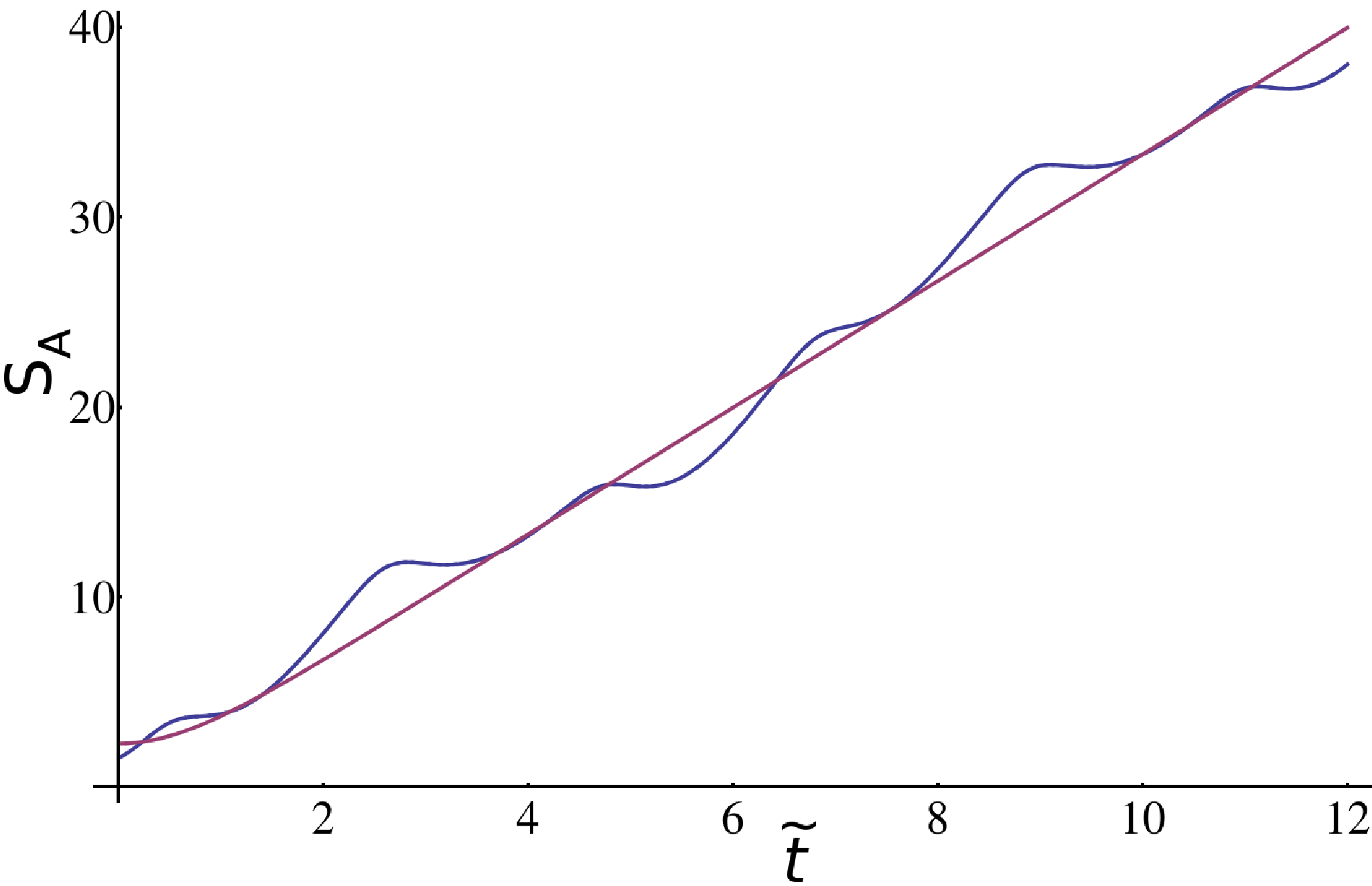
7 Entropy

As discussed in previous sections, our solutions of Section 2.3 are characterized by a smooth, albeit undulating, horizon (see Figure 4). This allows us, following [27], to define a holographic entropy current. We will first review the equilibrium situation (static black string), and then describe the calculation for the general, time-dependent solution. We will include a comparison with CFT calculations in both cases.

7.1 Equilibrium

Bulk calculation:

In case $L={\bar{L}}=$ constant, our solutions represent BTZ black strings (5) with a horizon at $\lambda=\lambda_{0}$ . The horizon ${\cal H}$ is a two-dimensional null surface, described by the metric

ds^{2}|_{{\cal H}}\equiv H_{\mu\nu}dx^{\mu}dx^{\nu}=\left(\sqrt{L}dv/2-\sqrt{{\bar{L}}}dw/2\right)^{2}

(64)

Since the normal to ${\cal H}$ at any point, given by $n^{M}=\partial^{M}\lambda(M=\{\lambda,v,w\})$ , also lies on ${\cal H}$ , ${\cal H}$ possesses a natural coordinate system $(\tau,\alpha)$ where $\alpha$ labels the one-parameter family of null geodesics, and $\tau$ measures the affine distance along the geodesics. In such a coordinate system, we get, by construction

ds^{2}|_{{\cal H}}=gd\alpha^{2}

(65)

The area 1-form and the entropy current on the horizon are defined by the equations [27] ²⁵²⁵ 25 Our convention for $\epsilon_{\mu\nu}$ is $\epsilon_{vw}=-1$ .,

\displaystyle a\equiv 4G_{3}\epsilon_{\mu\nu}J_{S}^{\mu}dx^{\nu}=\sqrt{g}d\alpha,

(66)

By inspection, from (64) and (65), we find the following expressions for the area-form and the entropy current

	$\displaystyle a$	$\displaystyle=\sqrt{L}dv/2-\sqrt{{\bar{L}}}dw/2$
	$\displaystyle J_{s}^{v}$	$\displaystyle=\frac{1}{8G_{3}}\sqrt{{\bar{L}}},\;J_{S}^{w}=\frac{1}{8G_{3}}\sqrt{L}$		(67)

The holographic entropy current on the boundary ${\cal B}$ is obtained by using a map $f:{\cal B}\to{\cal H}$ and pulling back the area-form (or alternatively the entropy current $J_{S,\mu}$ ) from the horizon to the boundary. It turns out ²⁶²⁶ 26 The map $f$ is defined by shooting ‘radial’ null geodesics inwards from the boundary, and is found to be of the form $f:(\lambda_{ir},v,w)\mapsto$ $(\lambda_{ir},v+C_{1},w+C_{2})$ . that the natural pull back retains the form of the area-form or entropy current, namely the expressions (67) still hold at the boundary.

To find the entropy density, we define the boundary coordinates $t=(v+w)/2,x=(v-w)/2$ (see Section 6), (so that (8) has the canonical form $-dt^{2}+dx^{2}$ ). With this the entropy density becomes

s\equiv J_{S}^{T}=\frac{1}{8G_{3}}\left(\sqrt{L}+\sqrt{{\bar{L}}}\right)

(68)

CFT calculation:

The entropy density from the Cardy formula is ²⁷²⁷ 27 Recall that both $T_{vv},T_{ww}$ are constant in this case. The more familiar form of (69), for a circular spatial direction of length $2\pi$ , is obtained by putting $S=2\pi s$ , $L_{0}=2\pi T_{vv}$ , and $\bar{L}_{0}=2\pi T_{ww}$ , which gives $S=2\pi(\sqrt{cL_{0}/6}+\sqrt{c{\bar{L}}_{0}/6}).$

s=\sqrt{c\pi T_{vv}/3}+\sqrt{c\pi T_{ww}/3}

(69)

Using the identification (44) and (9), we can easily see that the two expressions (68) and (69) exactly match.

7.2 New metrics: non-equilibrium entropy

Bulk calculation:

We will now follow a similar procedure as above, for the general solution in Section 2.3. We find that (in coordinate chart EF1)

ds^{2}|_{\mathcal{H}}=\frac{1}{4}d\alpha^{2}=\frac{1}{4}(\sqrt{L}G_{+}^{\prime}({\tilde{v}})d{\tilde{v}}-\sqrt{{\bar{L}}}G_{-}^{\prime}({\tilde{w}})d{\tilde{w}})^{2}

(70)

leading to the following area one form on the horizon

a=\frac{1}{2}\sqrt{L}G_{+}^{\prime}({\tilde{v}})d{\tilde{v}}-\frac{1}{2}\sqrt{{\bar{L}}}G_{-}^{\prime}({\tilde{w}})d{\tilde{w}}

(71)

Note that this could alternatively be obtained from the area form in (67) by a diffeomorphism. The resulting expression for the entropy current, following the steps above, is

{\tilde{J}}_{s}^{{\tilde{v}}}=\frac{1}{8G_{3}}\sqrt{{\bar{L}}}G^{\prime}_{-}({\tilde{w}}),\;{\tilde{J}}_{S}^{{\tilde{w}}}=\frac{1}{8G_{3}}\sqrt{L}G^{\prime}_{+}({\tilde{v}})

(72)

Let us define, as before, the spacetime coordinates as $\tilde{x},\tilde{t}$ with $(\tilde{v},\tilde{w})$ = $\tilde{t}\pm\tilde{x}$ . The entropy density is then given by

\tilde{s}={\tilde{J}}_{S}^{\tilde{t}}=\frac{1}{4G_{3}}\bigg(\frac{1}{2}\sqrt{L}G_{+}^{\prime}({\tilde{v}})+\frac{1}{2}\sqrt{\bar{L}}G_{-}^{\prime}({\tilde{w}})\bigg)

(73)

Note that the entropy current is divergenceless

\partial_{\mu}{{\tilde{J}}}^{\mu}_{S}=\partial_{{\tilde{v}}}{{\tilde{J}}}^{{\tilde{v}}}_{S}+\partial_{{\tilde{w}}}{\tilde{J}}^{{\tilde{w}}}_{S}=0

(74)

This has two implications:

1.

No dissipation: We have entropy transfers between different regions with no net entropy loss or production (see Figure 6).

Figure 6: The undulating horizon of Figure 2 leads to the non-trivial entropy current (73). In this figure, we plot the entropy density $\tilde{s}$ as a function of ${\tilde{v}},{\tilde{w}}$ for the right CFT. Note that although the entropy density fluctuates, the entropy flow here is such that there is no net entropy production (or destruction) (see Eq. (74)).

Total entropy is not changed by the conformal transformation: The other implication is that the integrated entropy over a space-like (or null) slice $\Sigma$

\tilde{S}=\int_{\Sigma}\epsilon_{\mu\nu}J_{S}^{\mu}d\sigma^{\nu}

(75)

is independent of the choice of the slice. In particular, choosing the slice to be $\Sigma_{0}:t=v+w=0$ , we get

	$\displaystyle\tilde{S}$	$\displaystyle=\frac{1}{8G_{3}}\ \int_{\Sigma_{0}}\left(\sqrt{L}G^{\prime}_{+}({\tilde{v}})d{\tilde{v}}-\sqrt{{\bar{L}}}G_{-}^{\prime}({\tilde{w}})d{\tilde{w}}\right)=\frac{1}{8G_{3}}\ \int_{\Sigma_{0}}\left(\sqrt{L}dv-\sqrt{{\bar{L}}}dw\right)$		(76)
		$\displaystyle=\frac{1}{8G_{3}}\ \int dx\left(\sqrt{L}+\sqrt{{\bar{L}}}\right)=\int dx\ s=S$		(77)

Hence although the entropy density is clearly transformed, the total entropy is not changed by the conformal transformation.

CFT calculation:

In a non-equilibrium situation, there is no natural notion of an entropy. However under the adiabatic approximation, the instantaneous eigenstates of a time-dependent Hamiltonian are a fair representation of the actual time-dependent wave functions. The consequent energy level density can thus be used to define an approximate time-dependent entropy. Generalizing this principle to slow time and space variations, and applying this to the stress tensor, one expects a space-time dependent version of (69), namely

\tilde{s}=\sqrt{\frac{\pi c}{3}\tilde{T}_{{\tilde{v}}{\tilde{v}}}}+\sqrt{\frac{\pi c}{3}\tilde{T}_{{\tilde{w}}{\tilde{w}}}}

(78)

where the stress tensors are given by (42). Since we have made the adiabatic approximation, we expect the above formula to be valid only up to the leading order of space and time derivatives. Under this approximation, we have

\displaystyle 8\pi G_{3}T_{{\tilde{v}}{\tilde{v}}}

\displaystyle=\frac{L}{4}G_{+}^{\prime}({\tilde{v}})^{2},\quad 8\pi G_{3}T_{{\tilde{w}}{\tilde{w}}}=\frac{{\bar{L}}}{4}G_{-}^{\prime}({\tilde{w}})^{2}

(79)

which exactly agrees with the holographic entropy density in (73). ²⁸²⁸ 28 Note that throughout this paper, we have not used the adiabatic approximation anywhere else. Thus, it is unsatisfactory to use this approximation here. It is, in fact, tempting to believe that the entropy density in (73), and not that in (78), actually gives the CFT entropy in general; however, this requires more investigation.

Total entropy for ${\cal H}_{R}$ is unchanged by the conformal transformation:

Under the conformal transformation (35), the reduced density matrix $\rho_{R}$ is changed by a unitary transformation:

\rho_{R}=\text{Tr}_{{\cal H}_{L}}|\psi\rangle\langle\psi|=U_{R}\,\rho_{0,R}\,U_{R}^{\dagger},\kern 10.0pt\rho_{0,R}=\text{Tr}_{{\cal H}_{L}}|\psi_{0}\rangle\langle\psi_{0}|

(80)

The total entropy of the system after the transformation is given by the von Neumann entropy $\tilde{S}=-\text{Tr}\rho_{R}\ln\rho_{R}$ which, therefore, is equal to the entropy before; it is unchanged by the unitary transformation.

8 Conclusion and open questions

In this paper we have solved the boundary value problem for 3D gravity (with $\Lambda<0$ ) with independent boundary data on two asymptotically AdS₃ exterior geometries. The boundary data, specified in the form of arbitrary holographic stress tensors, yields spacetimes with wormholes, i.e. with exterior regions connected across smooth horizons. The explicit metrics are constructed by the technique of solution generating diffeomorphisms (SGD) from the eternal BTZ black string. By using the fact that the SGD’s reduce to conformal transformations at both boundaries, we claim that the dual CFT states are specific time-dependent entangled states which are conformal transformations of the standard thermofield double. We compute various correlators and a dynamical entanglement entropy, in the bulk and in the CFT, to provide evidence for the duality. We also arrive at an expression for a non-equilibrium entropy function from the area-form on the horizon of these geometries.

Our work has implications for a number of other issues. We briefly discuss two of them below; a detailed study of these is left to future work.

8.1 ER=EPR

As mentioned above, our work constructs an infinite family of AdS-CFT dual pairs in which quantum states entangling two CFTs are holographically dual to spacetimes containing a wormhole region which connects the two exteriors. Both the quantum states and the wormhole geometries are explicitly constructed (see eqns. (29) and (13,21)). Our examples generalize the construction in [13, 14, 15]²⁹²⁹ 29 See [1, 5, 10] (for other remarks on unitary transformations of the thermofield double and related geometries see [5, 7, 10, 11, 12]) and provide an infinite family of examples of the relation ER=EPR, proposed in [1]. Since this relation has been extensively discussed and debated in the literature ([5, 10, 11, 12]), we would like to make some specific points pertaining to some of these discussions.

RR correlators vs RL correlators

It has been argued in [12],[5] and [10] that for typical entangled states connecting two CFTs, $\cal{H}_{R}$ and $\cal{H}_{L}$ , correlators involving operators on the left and the right are suppressed relative to those involving operators all on the right. In particular, according to [12], correlators of the form $\langle O_{R}O_{L}\rangle$ are of the order $e^{-S}\langle O_{R}O_{R}\rangle$ , where $S$ is the entropy of the right sided Hilbert space.

In Section 5 we have computed general two-point functions, both of the kind $\langle O_{R}(P)O_{R}(Q)\rangle$ and $\langle O_{R}(P)O_{L}(Q^{\prime})\rangle$ .³⁰³⁰ 30 We use unprimed labels for operators on the right and primed labels for those on the left. In case of the eternal BTZ (dual to the standard thermofield double), an inspection of (46) and (48) suggests that as the boundary point ${\bf P}$ goes off to infinity, the $\cosh$ and $\sinh$ factors tend to be equal, thus $L({\bf P},{\bf Q})\approx L({\bf P},{\bf Q}^{\prime})$ , thus there is no extra suppression in the two-sided correlator $\langle O_{R}\,O_{L}\rangle$ . Of course, such a statement, regarding the standard thermofield double, has been regarded as somewhat of a special nature.

We are therefore naturally led to ask: what happens in case of the new solutions found in this paper? The geodesic lengths $L({\bf P},{\bf Q})$ and $L({\bf P},{\bf Q}^{\prime})$ are now given by (50) and (). Once again, if the point P goes off towards the boundary of the Poincare plane, ${\tilde{v}}\to\infty$ . Hence $G_{+}({\tilde{v}})\to\infty$ (since $G_{+}$ is a monotonically increasing function). Hence, both the geodesic lengths approach each other. Thus, we do not see any peculiar additional suppression, even for our general entangled state, arising when the second point of the correlation function is moved from the right to the left CFT.

On the genericity of our family of examples

We start with the following Lemma.

Lemma: Any state $\in{\cal H}\otimes{\cal H}$ ,

|\Psi\rangle=\sum_{i,j}C_{ij}|i\rangle|j\rangle,\kern 5.0ptC_{ij}\in{\mathbb{C}},

(81)

can be expressed in the form

|\Psi\rangle=\sum_{i,j,n}e^{-\lambda_{n}}U_{L,in}U_{R,jn}|n\rangle|n\rangle

(82)

where $U_{R},U_{L}$ are two unitary operators and $\lambda_{n}\geq 0$ .

Proof: Using the canonical map ${\cal H}\otimes{\cal H}$ $\to{\cal H}\otimes{\cal H}^{*}$ , we can regard the above state $|\Psi\rangle$ as an operator ${\bf\Psi}$ in ${\cal H}$ , with matrix elements $C_{ij}$ . Using the singular value decomposition theorem on a general complex matrix, we can write $C=U_{L}DU_{R}^{\dagger}$ where $D$ is a diagonal matrix with real, non-negative entries. By denoting $D$ as diag[ $e^{-\lambda_{n}}$ ], we get (82).

The state (82) can be regarded as a thermofield double with Hamiltonian $H=$ $\sum_{n}\lambda_{n}/\beta$ $|n\rangle\langle n|$ transformed by unitary operators $U_{L}$ on the left and by $U_{R}$ on the right. Thus, the above Lemma suggests that the most general entangled state (81) can be written as a unitary transformation of some thermofield double state. Now, note that the state (82) is of the same general form as that of (29) discussed in this paper. Are our states (29) the most general entangled states then?

The answer is no, since the $U_{L,R}$ we use are made of Virasoro generators (see Appendix E), and are not the most general unitaries of (82). However, in spite of this restriction, it is clear that the states (29) do form a fairly general class. Furthermore, if the states (82) are states in which only the stress tensor is excited, then indeed these states are all contained in our class of states (29). ³¹³¹ 31 If a CFT dual to pure gravity were to exist, then our states (29) in such a theory would indeed be the most general state of the form (81). However, such a unitary theory is unlikely to exist [32, 33], although chiral gravity theories which are dual to CFTs with only the Virasoro operator have been suggested (see, e.g. [34]). We would like to thank Justin David for illuminating discussions on this point.

Weakly entangled states

To assess the genericity of our states, we ask a different question now: do our set of states (29), which are all explicitly dual to wormholes, include those with a very small entanglement entropy $S$ for a given energy $E$ ?³²³² 32 This question was suggested to us by Sandip Trivedi. The answer to this question turns out to be yes. As we have noted in the remarks around (77) and (80), the entropy $S$ , which is actually the entanglement entropy of the right Hilbert space, is the same for all our states. However, the same manipulations as in (77) shows that the energy of these states are not the same; indeed by choosing the derivatives $G_{\pm}^{\prime}$ to be large, we can make the energy of the transformed state to be much larger than that of the standard thermofield double. Stated in another way, for states of a given energy, our set of states includes states with entanglement entropy much less than that of the thermofield double. This is consistent with the proposal of [1] that even a small entanglement is described by a wormhole geometry.

8.2 Generalizations and open questions

It would be interesting to rephrase the results in this paper in terms of the $SL(2,R)\times SL(2,R)$ Chern-Simons formulation [35] of three-dimensional gravity. By the arguments in [35], all diffeomorphisms (together with appropriate local Lorentz rotations) can be understood as gauge transformations of the Chern-Simons theory. The Chern-Simons formulation has been extended to the gauge group $SL(N,R)$ $\times$ $SL(N,R)$ to describe higher spin theories [16, 36]. It would be interesting to see whether the nontrivial gauge transformations in our paper generalizes to these higher gauge groups, and hence to higher spin theories. A possible application of our methods in this case would be to compute HEE by the prescriptions in [37] and [38] in the nontrivial higher spin geometries³³³³ 33 We thank Rajesh Gopakumar for a discussion on this issue.. We hope to come back to this issue shortly.

The solutions presented in this paper are generated by SGDs which can be regarded as forming a group ( $\widetilde{\rm Vir}$ $\times$ $\widetilde{\rm Vir}$ )_L $\times$ ( $\widetilde{\rm Vir}$ $\times$ $\widetilde{\rm Vir}$ )_R. Here the first $\widetilde{\rm Vir}$ denotes a group of SGDs which is parametrized by the function $G_{+}$ , and so on. As we emphasized in (80), the reduced density matrix on the right $\rho_{R}$ undergoes a unitary transformation under this group of transformations, leaving the entropy unaltered. The family of pure states (29) considered in this paper can, therefore, be considered as an infinite family of purifications of the class of density matrices $\rho_{R}$ ; it would be interesting to see if these can be regarded as ‘micro-states’ which can ‘explain’ the entropy of $\rho_{R}$ . We hope to return to this issue shortly.

It would also be interesting to use our work to explicitly study various types of holographic quantum quenches involving quantum states entangling two CFTs.³⁴³⁴ 34 For a single CFT, a similar computation was done in, e.g., [22, 39]. It would be of particular interest to study limiting cases of our solutions which correspond to shock-wave geometries.

Acknowledgement

We would like to thank Atish Dabholkar, Justin David, Avinash Dhar, Rajesh Gopakumar, Juan Maldacena, Shiraz Minwalla, Suvrat Raju, Ashoke Sen, Lenny Susskind, Sandip Trivedi, Tomonori Ugajin and Spenta Wadia for many useful discussions during the course of this work. R.S. would like to thank Sachin Jain, Nilay Kundu and V. Umesh for discussions. We are grateful to Justin David, Avinash Dhar, Rajesh Gopakumar, Juan Maldacena, Lenny Susskind and Spenta Wadia for important feedbacks on the manuscript.

Appendix

Appendix A Coordinate systems for the eternal BTZ geometry

As we explained in the Introduction, the metric (1) describes only the region exterior to the black hole horizon (3). As is well-known, for constant ( $L,{\bar{L}}$ ), (1) describes a standard BTZ black hole with mass $M$ and angular momentum $J$ given by

L=8G_{3}(M+J),\;{\bar{L}}=8G_{3}(M-J)

(83)

In this section we will describe various coordinate systems for this case. In particular, we will describe the five coordinate charts of Figure 12 which cover our spacetime.

A.1 Eddington-Finkelstein coordinates

EF1 (Right Exterior + Black Hole Interior)

For a black hole with constant mass and angular momentum, it is straightforward to find a coordinate transformation from the ( $z,x_{+},x_{-}$ ) coordinates to a set of Eddington Finkelstein coordinates which we denote by EF1 ( $\lambda,v,y$ )

x_{+}=v-\frac{1}{2\sqrt{L}}\log\bigg(\frac{\lambda-\lambda_{0}}{\lambda+\lambda_{0}}\bigg),\hskip 5.69046ptx_{-}=y+\sqrt{\frac{L}{{\bar{L}}}}v-\frac{1}{2\sqrt{{\bar{L}}}}\log\bigg(\frac{\lambda^{2}-\lambda_{0}^{2}}{4{\bar{L}}}\bigg)

(84)

z=\sqrt{\frac{2}{\lambda_{0}^{2}}\bigg(\lambda-\sqrt{\lambda^{2}-\lambda_{0}^{2}}\bigg)}

(85)

Under these transformations, we obtain the following metric

\displaystyle ds^{2}=-\frac{2}{{\bar{L}}}\lambda_{0}(\lambda-\lambda_{0})dv^{2}+\frac{1}{\sqrt{{\bar{L}}}}dvd\lambda+\frac{{\bar{L}}}{4}dy^{2}-(\lambda-\lambda_{0})dvdy

(86)

The horizon (3) of the metric (1) is now located at $\lambda_{0}=\sqrt{L{\bar{L}}}/2$ . The metric is obviously smooth and describes the black hole interior.³⁵³⁵ 35 It develops a coordinate singularity at the inner horizon $\lambda=-\lambda_{0}$ ; we do not discuss interpolation beyond the inner horizon in this paper, although it can be easily done. In any case, there are strong reasons to believe that generically, the inner horizon and the associated exotic feature of infinitely repeating universes are unstable against even infinitesimal perturbations. To achieve a symmetry between the boundary coordinates, we find it convenient to make one further coordinate transformation from $y$ to $w$

y=w-\sqrt{\frac{L}{{\bar{L}}}}v+\frac{1}{\sqrt{{\bar{L}}}}\log\bigg(\frac{\lambda+\lambda_{0}}{2\sqrt{{\bar{L}}}}\bigg)

(87)

In these new coordinates ( $\lambda,v,w$ ), the metric becomes

\displaystyle ds^{2}=\frac{d\lambda^{2}}{4(\lambda+\lambda_{0})^{2}}+\frac{L}{4}dv^{2}+\frac{{\bar{L}}}{4}dw^{2}-\lambda dvdw+\frac{\sqrt{L}}{2(\lambda+\lambda_{0})}dvd\lambda+\frac{\sqrt{{\bar{L}}}}{2(\lambda+\lambda_{0})}dwd\lambda,

(88)

which is clearly symmetric between the ‘boundary coordinates’ $v$ and $w$ .

EF2 (Left Exterior + Black Hole Interior)

We can invent a second set of coordinate transformations starting from the metric in the ( $z,x_{+},x_{-}$ ) coordinates which would describe the left exterior region of the black hole along with the interior. This transformation is the following

x_{+}=u+\frac{1}{2\sqrt{L}}\log\bigg(\frac{\lambda_{1}-\lambda_{0}}{\lambda_{1}+\lambda_{0}}\bigg),\hskip 5.69046ptx_{-}=y_{1}+\sqrt{\frac{L}{{\bar{L}}}}u+\frac{1}{2\sqrt{{\bar{L}}}}\log\bigg(\frac{\lambda_{1}^{2}-\lambda_{0}^{2}}{4{\bar{L}}}\bigg)

(89)

z=\sqrt{\frac{2}{\lambda_{0}^{2}}\bigg(\lambda_{1}-\sqrt{\lambda_{1}^{2}-\lambda_{0}^{2}}\bigg)}

(90)

The Eddington-Finkelstein metric obtained via this transformation is

\displaystyle ds^{2}=-\frac{2}{{\bar{L}}}\lambda_{0}(\lambda_{1}-\lambda_{0})du^{2}-\frac{1}{\sqrt{\bar{L}}}dud\lambda_{1}+\frac{{\bar{L}}}{4}dy_{1}^{2}-(\lambda_{1}-\lambda_{0})dudy_{1}

(91)

As before, we make a further coordinate transformation $y_{1}$ to $\omega$

y_{1}=\omega-\sqrt{\frac{L}{{\bar{L}}}}u-\frac{1}{\sqrt{{\bar{L}}}}\log\bigg(\frac{\lambda_{1}+\lambda_{0}}{2\sqrt{{\bar{L}}}}\bigg)

(92)

to obtain the following metric in the ( $\lambda_{1},u,\omega$ ) coordinates

\displaystyle ds^{2}=\frac{d\lambda_{1}^{2}}{4(\lambda_{1}+\lambda_{0})^{2}}+\frac{L}{4}du^{2}+\frac{{\bar{L}}}{4}d\omega^{2}-\lambda_{1}dud\omega-\frac{\sqrt{{\bar{L}}}}{2(\lambda_{1}+\lambda_{0})}d\omega d\lambda_{1}-\frac{\sqrt{L}}{2(\lambda_{1}+\lambda_{0})}dud\lambda_{1}

(93)

EF3 (Left Exterior + White Hole Interior)

Starting from $(z,x_{+},x_{-})$ coordinates, we do the following transformations

x_{+}=v_{1}-\frac{1}{2\sqrt{L}}\log\bigg(\frac{\lambda_{1}-\lambda_{0}}{\lambda_{1}+\lambda_{0}}\bigg),\hskip 5.69046ptx_{-}=w_{1}-\frac{1}{2\sqrt{{\bar{L}}}}\log\bigg(\frac{\lambda_{1}-\lambda_{0}}{\lambda_{1}+\lambda_{0}}\bigg)

(94)

z=\sqrt{\frac{2}{\lambda_{0}^{2}}\bigg(\lambda_{1}-\sqrt{\lambda_{1}^{2}-\lambda_{0}^{2}}\bigg)}

(95)

The metric obtained is

ds^{2}=\frac{d\lambda_{1}^{2}}{4(\lambda_{1}+\lambda_{0})^{2}}+\frac{L}{4}dv_{1}^{2}+\frac{{\bar{L}}}{4}dw_{1}^{2}-\lambda_{1}dv_{1}dw_{1}+\frac{\sqrt{L}}{2(\lambda_{1}+\lambda_{0})}dv_{1}d\lambda_{1}+\frac{\sqrt{{\bar{L}}}}{2(\lambda_{1}+\lambda_{0})}dw_{1}d\lambda_{1}

(96)

This metric covers the left exterior and the white hole interior.

EF4(Right Exterior + White Hole Interior)

Starting from $(z,x_{+},x_{-})$ coordinates, we do the following transformations

x_{+}=u_{1}+\frac{1}{2\sqrt{L}}\log\bigg(\frac{\lambda-\lambda_{0}}{\lambda+\lambda_{0}}\bigg),\hskip 5.69046ptx_{-}=\omega_{1}+\frac{1}{2\sqrt{{\bar{L}}}}\log\bigg(\frac{\lambda-\lambda_{0}}{\lambda+\lambda_{0}}\bigg)

(97)

z=\sqrt{\frac{2}{\lambda_{0}^{2}}\bigg(\lambda-\sqrt{\lambda^{2}-\lambda_{0}^{2}}\bigg)}\\

(98)

The metric obtained is

ds^{2}=\frac{d\lambda^{2}}{4(\lambda+\lambda_{0})^{2}}+\frac{L}{4}du_{1}^{2}+\frac{{\bar{L}}}{4}d\omega_{1}^{2}-\lambda du_{1}d\omega_{1}-\frac{\sqrt{L}}{2(\lambda+\lambda_{0})}du_{1}d\lambda-\frac{\sqrt{{\bar{L}}}}{2(\lambda+\lambda_{0})}d\omega_{1}d\lambda

(99)

This metric covers the right exterior and the white hole interior.

Regions of Overlap

Right Exterior

The ‘Right Exterior’ region is described by both the EF1 $(\lambda,v,w)$ and EF4 $(\lambda,u_{1},\omega_{1})$ coordinates. These are related by the following smooth coordinate transformations

v=u_{1}+\frac{1}{\sqrt{L}}\log\bigg(\frac{\lambda-\lambda_{0}}{\lambda+\lambda_{0}}\bigg)\hskip 28.45274ptw=\omega_{1}+\frac{1}{\sqrt{{\bar{L}}}}\log\bigg(\frac{\lambda-\lambda_{0}}{\lambda+\lambda_{0}}\bigg)

(100)

Black Hole Interior

The ‘Black Hole Interior’ region is described by both the EF1 $(\lambda,v,w)$ and EF2 $(\lambda_{1},u,\omega)$ coordinates, which are related by the following smooth coordinate transformations

v=u+\frac{1}{\sqrt{L}}\log\bigg(\frac{\lambda_{0}-\lambda_{1}}{\lambda_{0}+\lambda_{1}}\bigg),\hskip 28.45274ptw=\omega+\frac{1}{\sqrt{{\bar{L}}}}\log\bigg(\frac{\lambda_{0}-\lambda_{1}}{\lambda_{0}+\lambda_{1}}\bigg),\quad\lambda_{1}=\lambda

(101)

Left Exterior

The ‘Left Exterior’ region is described by both the EF2 $(\lambda_{1},u,\omega)$ and EF3 $(\lambda_{1},v_{1},\omega_{1})$ coordinates, which are related by the following smooth coordinate transformations:

v_{1}=u+\frac{1}{\sqrt{L}}\log\bigg(\frac{\lambda_{1}-\lambda_{0}}{\lambda_{1}+\lambda_{0}}\bigg)\hskip 28.45274ptw_{1}=\omega+\frac{1}{\sqrt{{\bar{L}}}}\log\bigg(\frac{\lambda_{1}-\lambda_{0}}{\lambda_{1}+\lambda_{0}}\bigg)

(102)

White Hole Interior

The ‘White Hole Interior’ finds a description in both the EF3 $(\lambda_{1},v_{1},\omega_{1})$ and EF4 $(\lambda,u_{1},\omega_{1})$ coordinates, which are related by the following smooth coordinate transformations:

v_{1}=u_{1}+\frac{1}{\sqrt{L}}\log\bigg(\frac{\lambda_{0}-\lambda}{\lambda_{0}+\lambda}\bigg),\hskip 28.45274ptw_{1}=\omega_{1}+\frac{1}{\sqrt{{\bar{L}}}}\log\bigg(\frac{\lambda_{0}-\lambda_{1}}{\lambda_{0}+\lambda_{1}}\bigg),\quad\lambda=\lambda_{1}

(103)

A.2 Kruskal coordinates

The union of all the above coordinate patches, together with a neighbourhood (indicated by K5 in Fig 12) of the bifurcation surface (the meeting point of the past and future horizons in the Penrose diagram) can be described by a set of Kruskal coordinates, in which the metric reads

ds^{2}=-\frac{1}{2\lambda_{0}}dUdV+\frac{1}{\sqrt{L}}UdVdy+\frac{{\bar{L}}}{4}dy^{2}

(104)

The coordinate transformation between various EF coordinates and the Kruskal coordinates are given below.

1. Right exterior + Black Hole Interior : EF1 to Kruskal

The transformation from EF1 to the $(U,V,y)$ coordinates is

U=-\exp(-\sqrt{L}v)(\lambda-\lambda_{0}),\hskip 5.69046ptV=\exp(\sqrt{L}v),\hskip 5.69046pty=w-\sqrt{\frac{L}{{\bar{L}}}}v+\frac{1}{\sqrt{{\bar{L}}}}\log\bigg(\frac{\lambda+\lambda_{0}}{2\sqrt{{\bar{L}}}}\bigg)

(105)

In the ‘Right Exterior’ region, $\lambda>\lambda_{0}$ , while in the ‘Black Hole Interior’, $\lambda<\lambda_{0}$ . The above transformations give us the metric (104) in both the regions.

2. Left Exterior + Black Hole Interior : EF2 to Kruskal

The transformation from EF2 to $(U,V,y)$ coordinates is

U=\exp(-\sqrt{L}u)(\lambda_{1}+\lambda_{0}),\hskip 5.69046ptV=-\exp(\sqrt{L}u)\frac{\lambda_{1}-\lambda_{0}}{\lambda_{1}+\lambda_{0}},\hskip 5.69046pty=\omega-\sqrt{\frac{L}{{\bar{L}}}}u+\frac{1}{\sqrt{{\bar{L}}}}\log(\lambda_{1}+\lambda_{0})

(106)

with,

y_{1}=y-\frac{2}{\sqrt{{\bar{L}}}}\log\bigg(\frac{\lambda_{1}+\lambda_{0}}{2\sqrt{{\bar{L}}}}\bigg)

(107)

In the ‘Black Hole Interior’ $\lambda_{1}<\lambda_{0}$ , while in the ‘Left Exterior’ region $\lambda_{1}>\lambda_{0}$ . These coordinate transformations give us the metric (104) in both the regions.

3. Left Exterior + White Hole Interior : EF3 to Kruskal

The transformations from EF3 to the $(U,V,y)$ coordinates is

U=\exp(-\sqrt{L}v_{1})(\lambda_{1}-\lambda_{0}),\hskip 5.69046ptV=-\exp(\sqrt{L}v_{1}),\hskip 5.69046pty=w_{1}-\sqrt{\frac{L}{{\bar{L}}}}v_{1}+\frac{1}{\sqrt{{\bar{L}}}}\log\bigg(\frac{\lambda_{1}+\lambda_{0}}{2\sqrt{{\bar{L}}}}\bigg)

(108)

In the ‘Left Exterior’ region $\lambda_{1}>\lambda_{0}$ , while in the ‘White Hole Interior’, $\lambda_{1}<\lambda_{0}$ . These transformations give us the metric (104) in both the regions.

4. Right Exterior + White Hole Interior : EF4 to Kruskal

The transformation from EF4 to the $(U,V,y)$ coordinates is

U=-\exp(-\sqrt{L}u_{1})(\lambda+\lambda_{0}),\hskip 5.69046ptV=\exp(\sqrt{L}u_{1})\frac{\lambda-\lambda_{0}}{\lambda+\lambda_{0}},\hskip 5.69046pty=\omega_{1}-\sqrt{\frac{L}{{\bar{L}}}}u_{1}+\frac{1}{\sqrt{{\bar{L}}}}\log(\lambda+\lambda_{0})

(109)

with,

y_{1}=y-\frac{2}{\sqrt{{\bar{L}}}}\log\bigg(\frac{\lambda_{1}+\lambda_{0}}{2\sqrt{{\bar{L}}}}\bigg)

(110)

In the ‘White Hole Interior’ $\lambda<\lambda_{0}$ , while in the ‘Right Exterior’ region $\lambda>\lambda_{0}$ . The above transformations give us the metric (104) in both the regions.

A.3 Poincare

In this section we show how the EF1, EF2 coordinates can, in fact, be obtained from Poincare coordinates $\zeta,X_{\pm}=X_{0}\pm X_{1}$ , in terms of which the metric is written as

ds^{2}=\frac{1}{\zeta^{2}}(d\zeta^{2}-dX_{+}dX_{-})

(111)

We will choose $L={\bar{L}}$ for simplicity, so $\lambda_{0}=L/2$ .

The coordinate transformation from $X_{\pm},\zeta$ to the EF1 coordinates is given by

\displaystyle v

\displaystyle=

\displaystyle\frac{\log(X_{+})}{\sqrt{L}},\;w=-\frac{1}{\sqrt{L}}\log\left(\frac{-X_{+}X_{-}+\zeta^{2}}{X_{+}}\right),\;\frac{\lambda}{\lambda_{0}}=\frac{-2X_{+}X_{-}+\zeta^{2}}{\zeta^{2}}\

(112)

whereas the coordinate transformation from $X_{\pm},\zeta$ to the EF2 coordinates is given by

\displaystyle u

\displaystyle=

\displaystyle\frac{1}{\sqrt{L}}\log\left(\frac{-X_{+}X_{-}+\zeta^{2}}{X_{-}}\right),\;\omega=-\frac{\log(X_{-})}{\sqrt{L}},\;\frac{\lambda_{1}}{\lambda_{0}}=\frac{-2X_{+}X_{-}+\zeta^{2}}{\zeta^{2}}\

(113)

There are similar coordinate transformations between the other charts EF3/4 and Poincare.³⁶³⁶ 36 As explained in [14] , it is possible to describe the BTZ black string in terms of a single Poincare chart. The BTZ black hole is a quotient of AdS₃, which in appropriate coordinates [40] corresponds to the periodic identification of the spatial direction; the BTZ string discussed in this paper is obtained by decompactifying the spatial circle, which gives back AdS₃.

Appendix B The new metrics in the charts EF3 and EF4

	$\displaystyle\hbox{EF3:}~~ds^{2}$	$\displaystyle=\frac{1}{B^{2}}\left[d{\tilde{\lambda}}_{1}^{2}+A_{+}^{2}d{\tilde{v}}_{1}^{2}+A_{-}^{2}d{\tilde{w}}_{1}^{2}+2A_{+}d{\tilde{u}}_{1}d{\tilde{\lambda}}_{1}+2A_{-}d{\tilde{w}}_{1}d{\tilde{\lambda}}_{1}\right.$
		$\displaystyle-\left.{\tilde{\lambda}}_{1}\bigg(B^{2}+2\bigg(A_{+}\frac{H_{-}^{\prime\prime}({\tilde{w}}_{1})}{H_{-}^{\prime}({\tilde{w}}_{1})}+A_{-}\frac{H_{+}^{\prime\prime}({\tilde{v}}_{1})}{H_{+}^{\prime}({\tilde{v}}_{1})}+{\tilde{\lambda}}\frac{H_{+}^{\prime\prime}({\tilde{v}}_{1})H_{-}^{\prime\prime}({\tilde{w}}_{1})}{H_{+}^{\prime}({\tilde{v}}_{1})H_{-}^{\prime}({\tilde{w}}_{1})}\bigg)\bigg)d{\tilde{w}}_{1}d{\tilde{v}}_{1}\right]$		(114)

where

\displaystyle A_{+}=\sqrt{L}H_{+}^{\prime}({\tilde{v}}_{1})({\tilde{\lambda}}_{1}+{\tilde{\lambda}}_{10})-{\tilde{\lambda}}_{1}\frac{H_{+}^{\prime\prime}({\tilde{v}}_{1})}{H_{+}^{\prime}({\tilde{v}}_{1})},\;A_{-}=\sqrt{{\bar{L}}}H_{-}^{\prime}({\tilde{w}}_{1})({\tilde{\lambda}}_{1}+{\tilde{\lambda}}_{10})-{\tilde{\lambda}}_{1}\frac{H_{-}^{\prime\prime}({\tilde{w}}_{1})}{H_{-}^{\prime}({\tilde{w}}_{1})},\;B=2({\tilde{\lambda}}_{1}+{\tilde{\lambda}}_{10})

	$\displaystyle\hbox{EF4}:~~ds^{2}$	$\displaystyle=\frac{1}{B^{2}}\left[d{\tilde{\lambda}}^{2}+A_{+}^{2}d{\tilde{u}}_{1}^{2}+A_{-}^{2}d{\tilde{\omega}}_{1}^{2}-2A_{+}d{\tilde{u}}_{1}d{\tilde{\lambda}}-2A_{-}d{\tilde{\omega}}_{1}d{\tilde{\lambda}}\right.$
		$\displaystyle-\left.{\tilde{\lambda}}\bigg(B^{2}-2\bigg(A_{+}\frac{G_{-}^{\prime\prime}({\tilde{\omega}}_{1})}{G_{-}^{\prime}({\tilde{\omega}}_{1})}+A_{-}\frac{G_{+}^{\prime\prime}({\tilde{u}}_{1})}{G_{+}^{\prime}({\tilde{u}}_{1})}-{\tilde{\lambda}}\frac{G_{+}^{\prime\prime}({\tilde{u}}_{1})G_{-}^{\prime\prime}({\tilde{\omega}}_{1})}{G_{+}^{\prime}({\tilde{u}}_{1})G_{-}^{\prime}({\tilde{\omega}}_{1})}\bigg)\bigg)d{\tilde{\omega}}_{1}d{\tilde{u}}_{1}\right]$		(115)

where

\displaystyle A_{+}=\sqrt{L}G_{+}^{\prime}({\tilde{u}}_{1})({\tilde{\lambda}}+{\tilde{\lambda}}_{0})+{\tilde{\lambda}}\frac{G_{+}^{\prime\prime}({\tilde{u}}_{1})}{G_{+}^{\prime}({\tilde{u}}_{1})},\;A_{-}=\sqrt{{\bar{L}}}G_{-}^{\prime}({\tilde{\omega}}_{1})({\tilde{\lambda}}+{\tilde{\lambda}}_{0})+{\tilde{\lambda}}\frac{G_{-}^{\prime\prime}({\tilde{\omega}}_{1})}{G_{-}^{\prime}({\tilde{\omega}}_{1})},\;B=2({\tilde{\lambda}}+{\tilde{\lambda}}_{0})

Appendix C UV/IR cutoffs in EF coordinates

From AdS/CFT it is well-known that in a Fefferman-Graham coordinate system such as in (1), an IR cutoff surface $z=\epsilon$ in the asymptotically AdS spacetime corresponds to a UV cutoff $\epsilon$ in the CFT. We wish to express the IR cutoff in the geometry in terms of the EF coordinates. By using the relation

z=\sqrt{\frac{2}{\lambda_{0}^{2}}\bigg(\lambda-\sqrt{\lambda^{2}-\lambda_{0}^{2}}\bigg)}

(116)

we clearly see that $z=\epsilon$ for $\epsilon$ small, corresponds to $\lambda=1/\epsilon^{2}$ .

Appendix D An alternative to Banados’ metric

In a beautiful paper [22], Roberts showed that the Banados metric (1) can be obtained from the Poincare metric (111) by a Brown-Henneaux type diffeomorphism (an ‘SGD’ in the language of our paper), given by

	$\displaystyle X_{\pm}$	$\displaystyle=$	$\displaystyle f_{\pm}(x_{\pm})+\frac{2z^{2}f_{\pm}^{\prime}(x_{\pm})^{2}f_{\mp}^{\prime\prime}(x_{\mp})}{8f_{\pm}^{\prime}(x_{\pm})f_{\mp}^{\prime}(x_{\mp})-z^{2}f_{\pm}^{\prime\prime}(x_{\pm})f_{\mp}^{\prime\prime}(x_{\mp})}$
	$\displaystyle\vskip 142.26378pt\zeta$	$\displaystyle=$	$\displaystyle z\ \frac{\left(4f_{+}^{\prime}(x_{+})f_{-}^{\prime}(x_{-})\right)^{\frac{3}{2}}}{8f_{+}^{\prime}(x_{+})f_{-}^{\prime}(x_{-})-z^{2}f_{+}^{\prime\prime}(x_{+})f_{-}^{\prime\prime}(x_{-})}$		(117)

It was shown in [22] that the above diffeomorphism reduces to a conformal transformation on the boundary, with the the following asymptotic form (as z $\rightarrow$ 0)

	$\displaystyle X_{\pm}$	$\displaystyle=$	$\displaystyle f_{\pm}(x_{\pm})+O(z^{2})\vskip 426.79134pt$
	$\displaystyle\zeta$	$\displaystyle=$	$\displaystyle z\sqrt{f_{+}^{\prime}(x_{+})f_{-}^{\prime}(x_{-})}+O(z^{3})$		(118)

It was also shown in this paper that $L(x_{+}),{\bar{L}}(x_{-})$ appearing in (1) can be obtained from the zero stress tensor through the conformal transformation $f_{\pm}$ .

A different choice of gauge: The SGD (117) used by Roberts seems fairly involved compared to the ones we use in this paper, e.g. (12). Can we obtain the metric (1) by a simpler SGD similar to ours, which nevertheless has the same conformal asymptotic form (118)? The answer turns out to be yes. Indeed the simplest way of inventing such a transformation is to take the asymptotic form (118) and gauge fix all the higher order terms in $z$ to 0. We then have a new, exact transformation of the form

X_{\pm}=f_{\pm}(x_{\pm}),\hskip 28.45274pt\zeta=z\sqrt{f_{+}^{\prime}(x_{+})f_{-}^{\prime}(x_{-})}

(119)

Note the similarity with our SGDs, say (12) (recall that $z\sim 1/\sqrt{\lambda}$ near the boundary). (119) transforms the Poincare metric to

	$\displaystyle ds^{2}=$	$\displaystyle\frac{dz^{2}}{z^{2}}+\frac{f_{+}^{\prime\prime}(x_{+})}{zf_{+}^{\prime}(x_{+})}dx_{+}dz+\frac{f_{-}^{\prime\prime}(x_{-})}{zf_{-}^{\prime}(x_{-})}dx_{-}dz+\frac{1}{4}\left(\frac{f_{+}^{\prime\prime}(x_{+})^{2}}{f_{+}^{\prime}(x_{+})^{2}}dx_{+}^{2}+\frac{f_{-}^{\prime\prime}(x_{-})^{2}}{f_{-}^{\prime}(x_{-})^{2}}dx_{-}^{2}\right)$
		$\displaystyle-\left(\frac{2}{z^{2}}-\frac{f_{+}^{\prime\prime}(x_{+})f_{-}^{\prime\prime}(x_{-})}{2f_{+}^{\prime}(x_{+})f_{-}^{\prime}(x_{-})}\right)dx_{+}dx_{-}$		(120)

A priori this is a new metric different from (1). However, the holographic stress tensor [23] obtained from this metric is the same as obtained from (1) given by (42). As discussed in Section 2.5 and 2.5.1, the above metric and (1) differ only by a trivial diffeomorphism, and are hence essentially identical.³⁷³⁷ 37 Note that in this new metric (120), the position of the horizon is at $z=\infty$ . Of course, it can be brought to a finite value by an additional coordinate transformation involving the radial coordinate. Note that this example shows the enormous gauge ambiguity in the choice of a metric in AdS₃ (whose physical content is manifested in the boundary behaviour). Indeed, by the same token even the SGD’s employed in this paper are ambiguous; the solutions presented in Section 2 are one of a gauge equivalent class of metrics.

Appendix E Unitary realization of conformal transformation

Under a finite, non-trivial, holomorphic coordinate transformation, $w\rightarrow w^{\prime}=f(w)$ , the stress tensor of a 2D CFT transforms as

\tilde{T}(w^{\prime})=\bigg(\frac{\partial w^{\prime}}{\partial w}\bigg)^{-2}[T(w)-\frac{c}{12}S(w^{\prime},w)]

(121)

with the Schwarzian derivative S( $w^{\prime},w$ ) given by

S(w^{\prime},w)=\bigg(\frac{\partial^{3}w^{\prime}}{\partial w^{3}}\bigg)\bigg(\frac{\partial w^{\prime}}{\partial w}\bigg)^{-1}-\frac{3}{2}\bigg(\frac{\partial^{2}w^{\prime}}{\partial w^{2}}\bigg)^{2}\bigg(\frac{\partial w^{\prime}}{\partial w}\bigg)^{-2}

(122)

For an infinitesimal transformation $w\rightarrow w^{\prime}=f(w)=w+\epsilon(w)$ , the Schwarzian derivative turns out to be

S(w^{\prime},w)=\epsilon^{\prime\prime\prime}(w)+\mathcal{O}(\epsilon^{2})

(123)

The change in the stress tensor, under such a transformation, becomes

\delta T(w)\approx-\epsilon(w)T^{\prime}(w)-2\epsilon^{\prime}(w)T(w)-\frac{c}{12}\epsilon^{\prime\prime\prime}(w)+\mathcal{O}(\epsilon^{2})

(124)

Now, the Laurent expansion of $T(w)$ and $\epsilon(w)$ is

T(w)=\sum_{m=-\infty}^{\infty}\frac{L_{m}}{w^{m+2}}\hskip 56.9055pt\epsilon(w)=\sum_{m=-\infty}^{\infty}\epsilon_{m}w^{-m+1}

(125)

where $L^{\dagger}_{n}=L_{-n}$ , $\epsilon^{\dagger}_{n}=-\epsilon_{-n}$ and the $L_{n}$ ’s satisfy the Virasoro algebra

[L_{m},L_{n}]=(m-n)L_{m+n}+\frac{c}{12}m(m^{2}-1)\delta_{m+n,0}

(126)

Plugging (125) into (124), we get

\delta L_{m}=\sum_{n=-\infty}^{\infty}\bigg\{(m+n)L_{m-n}\epsilon_{n}+\frac{c}{12}n(n^{2}-1)\epsilon_{n}\delta_{m-n,0}\bigg\}

(127)

We wish to construct a unitary operator $U=U(\epsilon)$ which implements the above conformal transformations, namely that it satisfies

U(\epsilon)^{\dagger}L_{m}U(\epsilon)-L_{m}=\delta L_{m}+O(\epsilon^{2})

(128)

The required unitary operator, in fact, is

U(\epsilon)=\exp(\sum_{n=-\infty}^{\infty}\epsilon_{n}L_{-n})

(129)

The proof is straightforward. Note that the LHS of (128) becomes

(1-\sum_{n}\epsilon_{-n}L_{n})L_{m}(1+\sum_{n}\epsilon_{n}L_{-n})-L_{m}=-\sum_{n=-\infty}^{\infty}\epsilon_{-n}(L_{n}L_{m})+\sum_{n=-\infty}^{\infty}\epsilon_{n}(L_{m}L_{-n})+\mathcal{O}(\epsilon^{2})\

After flipping the sign of $n$ in the first sum, this becomes

\epsilon_{n}[L_{m},L_{-n}]

which reduces to the expression (127) upon using the Virasoro algebra (126).

Thus, we have explicitly constructed a unitary operator $U$ such that $U^{\dagger}T(w)U-T(w)$ is given by (124).

References

[1] J. Maldacena and L. Susskind, Cool Horizons for Entangled Black Holes, Fortsch.Phys. 61 (2013) pp. 781–811, [arXiv:1306.0533].
[2] A. Almheiri, D. Marolf, J. Polchinski, and J. Sully, Black Holes: Complementarity or Firewalls?, JHEP 1302 (2013) p. 062, [arXiv:1207.3123].
[3] A. Almheiri, D. Marolf, J. Polchinski, D. Stanford, and J. Sully, An Apologia for Firewalls, JHEP 1309 (2013) p. 018, [arXiv:1304.6483].
[4] S. L. Braunstein, S. Pirandola, and K. Å»yczkowski, Better Late than Never: Information Retrieval from Black Holes, Phys.Rev.Lett. 110 (2013), no. 10 p. 101301, [arXiv:0907.1190].
[5] S. H. Shenker and D. Stanford, Black holes and the Butterfly Effect, JHEP 1403 (2014) p. 067, [arXiv:1306.0622].
[6] M. Van Raamsdonk, Evaporating Firewalls, arXiv:1307.1796.
[7] D. Marolf and J. Polchinski, Gauge/Gravity Duality and the Black Hole Interior, Phys.Rev.Lett. 111 (2013) p. 171301, [arXiv:1307.4706].
[8] K. Papadodimas and S. Raju, State-Dependent Bulk-Boundary Maps and Black Hole Complementarity, Phys.Rev. D89 (2014) p. 086010, [arXiv:1310.6335].
[9] K. Papadodimas and S. Raju, The Black Hole Interior in AdS/CFT and the Information Paradox, Phys.Rev.Lett. 112 (2014) p. 051301, [arXiv:1310.6334].
[10] S. H. Shenker and D. Stanford, Multiple Shocks, arXiv:1312.3296.
[11] S. G. Avery and B. D. Chowdhury, No Holography for Eternal AdS Black Holes, arXiv:1312.3346.
[12] V. Balasubramanian, M. Berkooz, S. F. Ross, and J. Simon, Black Holes, Entanglement and Random Matrices, arXiv:1404.6198.
[13] J. M. Maldacena, Eternal Black Holes in Anti-de Sitter, JHEP 0304 (2003) p. 021, [hep-th/0106112].
[14] T. Hartman and J. Maldacena, Time Evolution of Entanglement Entropy from Black Hole Interiors, JHEP 1305 (2013) p. 014, [arXiv:1303.1080].
[15] P. Caputa, G. Mandal, and R. Sinha, Dynamical Entanglement Entropy with Angular Momentum and U(1) Charge, JHEP 1311 (2013) p. 052, [arXiv:1306.4974].
[16] M. Banados, Three-Dimensional Quantum Geometry and Black Holes, hep-th/9901148.
[17] R. K. Gupta and A. Mukhopadhyay, On the Universal Hydrodynamics of Strongly Coupled CFTs with Gravity Duals, JHEP 0903 (2009) p. 067, [arXiv:0810.4851].
[18] T. Regge and C. Teitelboim, Role of Surface Integrals in the Hamiltonian Formulation of General Relativity, Annals Phys. 88 (1974) p. 286.
[19] S. Wadia, Canonical Quantization of Non-Abelian Gauge Theory in the Schrodinger Picture: Applications to Monopoles and Instantons, Ph.D. Thesis (1979).
[20] J.-L. Gervais, B. Sakita, and S. Wadia, The Surface Term in Gauge Theories, Phys.Lett. B63 (1976) p. 55.
[21] J. D. Brown and M. Henneaux, Central Charges in the Canonical Realization of Asymptotic Symmetries: An Example from Three-Dimensional Gravity, Commun.Math.Phys. 104 (1986) pp. 207–226.
[22] M. M. Roberts, Time Evolution of Entanglement Entropy from a Pulse, JHEP 1212 (2012) p. 027, [arXiv:1204.1982].
[23] V. Balasubramanian and P. Kraus, A Stress Tensor for Anti-de Sitter Gravity, Commun.Math.Phys. 208 (1999) pp. 413–428, [hep-th/9902121].
[24] K. Skenderis and S. N. Solodukhin, Quantum Effective Action from the AdS / CFT Correspondence, Phys.Lett. B472 (2000) pp. 316–322, [hep-th/9910023].
[25] S. Ryu and T. Takayanagi, Holographic Derivation of Entanglement Entropy from AdS/CFT, Phys.Rev.Lett. 96 (2006) p. 181602, [hep-th/0603001].
[26] V. E. Hubeny, M. Rangamani, and T. Takayanagi, A Covariant Holographic Entanglement Entropy Proposal, JHEP 0707 (2007) p. 062, [arXiv:0705.0016].
[27] S. Bhattacharyya, V. E. Hubeny, R. Loganayagam, G. Mandal, S. Minwalla, et. al., Local Fluid Dynamical Entropy from Gravity, JHEP 0806 (2008) p. 055, [arXiv:0803.2526].
[28] S. Bhattacharyya, V. E. Hubeny, S. Minwalla, and M. Rangamani, Nonlinear Fluid Dynamics from Gravity, JHEP 0802 (2008) p. 045, [arXiv:0712.2456].
[29] J. Louko, D. Marolf, and S. F. Ross, On Geodesic Propagators and Black Hole Holography, Phys.Rev. D62 (2000) p. 044041, [hep-th/0002111].
[30] J. L. Cardy, Operator Content of Two-Dimensional Conformally Invariant Theories, Nucl.Phys. B270 (1986) pp. 186–204.
[31] P. Calabrese and J. L. Cardy, Evolution of entanglement entropy in one-dimensional systems, J.Stat.Mech. 0504 (2005) p. P04010, [cond-mat/0503393].
[32] A. Maloney and E. Witten, Quantum Gravity Partition Functions in Three Dimensions, JHEP 1002 (2010) p. 029, [arXiv:0712.0155].
[33] M. R. Gaberdiel, Constraints on Extremal Self-Dual CFTs, JHEP 0711 (2007) p. 087, [arXiv:0707.4073].
[34] H. Afshar, A. Bagchi, S. Detournay, D. Grumiller, S. Prohazka, et. al., Holographic Chern-Simons Theories, arXiv:1404.1919.
[35] E. Witten, (2+1)-Dimensional Gravity as an Exactly Soluble System, Nucl.Phys. B311 (1988) p. 46.
[36] A. Campoleoni, S. Fredenhagen, S. Pfenninger, and S. Theisen, Asymptotic symmetries of three-dimensional gravity coupled to higher-spin fields, JHEP 1011 (2010) p. 007, [arXiv:1008.4744].
[37] M. Ammon, A. Castro, and N. Iqbal, Wilson Lines and Entanglement Entropy in Higher Spin Gravity, JHEP 1310 (2013) p. 110, [arXiv:1306.4338].
[38] J. de Boer and J. I. Jottar, Entanglement Entropy and Higher Spin Holography in AdS₃, arXiv:1306.4347.
[39] T. Ugajin, Two dimensional quantum quenches and holography, arXiv:1311.2562.
[40] V. Balasubramanian, P. Kraus, and A. E. Lawrence, Bulk versus Boundary Dynamics in Anti-de Sitter Space-Time, Phys.Rev. D59 (1999) p. 046003, [hep-th/9805171].