We treat the interaction of the electron with the background ${\mathcal{L}}_{\rm BG}$ as perturbation and compute an $S$-matrix element for the $e^{+}e^{-}$ pair creation from the vacuum, $S\equiv\braket{e^{-}(\mbox{\boldmath$p$},s)\,e^{+}(\mbox{\boldmath$p$}^{\prime},s^{\prime});{\rm out}|{\rm vac;in}}=\bra{e^{-}(\mbox{\boldmath$p$},s)\,e^{+}(\mbox{\boldmath$p$}^{\prime},s^{\prime});{\rm in}}{\sf T}\exp[i\int d^{4}x{\mathcal{L}}_{\rm BG}]\ket{\rm vac;in}$, in the lowest order perturbation theory. The diagrammatic expression for the lowest-order contribution $S^{(1)}$ reads

	$\displaystyle S^{(1)}$	$\displaystyle\equiv\bra{e^{-}(\mbox{\boldmath$p$},s)\,e^{+}(\mbox{\boldmath$p$}^{\prime},s^{\prime});{\rm in}}i\int d^{4}x{\mathcal{L}}_{\rm BG}\ket{\rm vac;in}$
		$\displaystyle=\parbox{34.1433pt}{\includegraphics[width=68.2866pt]{fig1.eps}}\,.$		(2)

A straightforward calculation yields

	$\displaystyle S^{(1)}$	$\displaystyle=-i\int d^{4}x(e\bar{A}_{3}(x^{0}))\bra{e^{-}(\mbox{\boldmath$p$},s)\,e^{+}(\mbox{\boldmath$p$}^{\prime},s^{\prime}){\rm;in}}\bar{\psi}(x)\gamma^{3}\psi(x)\ket{\rm vac;in}$
		$\displaystyle=i\left[\int dx^{0}\left(e\bar{A}_{3}(x^{0})\right){\rm e}^{2ip_{0}x^{0}}\right]\big(\bar{u}(\mbox{\boldmath$p$},s)\gamma^{3}v(-\mbox{\boldmath$p$},s^{\prime})\big)\delta^{3}({\mbox{\boldmath$p$}}+{\mbox{\boldmath$p$}}^{\prime})$
		$\displaystyle=\frac{e\tilde{E}(2p_{0})}{2p_{0}}\;\big(\bar{u}(\mbox{\boldmath$p$},s)\gamma^{3}v(-\mbox{\boldmath$p$},s^{\prime})\big)\delta^{3}(\mbox{\boldmath$p$}+\mbox{\boldmath$p$}^{\prime})\,.$		(3)

Note that we have expanded the unperturbed operator $\psi$ as

$\displaystyle\psi(x)=\sum_{s}\int d^{3}\mbox{\boldmath$p$}\left[u(\mbox{\boldmath$p$},s)\frac{{\rm e}^{-i(p_{0}x^{0}-{\small\mbox{\boldmath$p\cdot x$}})}}{\sqrt{(2\pi)^{3}}}a(\mbox{\boldmath$p$},s)+v(\mbox{\boldmath$p$},s)\frac{{\rm e}^{i(p_{0}x^{0}-{\small\mbox{\boldmath$p\cdot x$}})}}{\sqrt{(2\pi)^{3}}}b^{\dagger}(\mbox{\boldmath$p$},s)\right]$

(4)

to get the second expression. Here $p_{0}=\sqrt{m^{2}+\mbox{\boldmath$p$}^{2}}$, the annihilation operators $a(\mbox{\boldmath$p$},s)$ for an electron and $b(\mbox{\boldmath$p$},s)$ for a positron satisfy the following anticommutation relations: $\big\{a(\mbox{\boldmath$p$},s),a^{\dagger}({\mbox{\boldmath$p$}^{\prime}},s^{\prime})\big\}=\big\{b(\mbox{\boldmath$p$},s),b^{\dagger}({\mbox{\boldmath$p$}^{\prime}},s^{\prime})\big\}=\delta_{ss^{\prime}}\delta^{3}(\mbox{\boldmath$p-p^{\prime}$})\,,\ (\text{otherwise})=0\,,$ and the Dirac spinors $u(\mbox{\boldmath$p$},s),v(\mbox{\boldmath$p$},s)$ are normalized as $u^{\dagger}(\mbox{\boldmath$p$},s)u(\mbox{\boldmath$p$},s^{\prime})=v^{\dagger}(\mbox{\boldmath$p$},s)v(\mbox{\boldmath$p$},s^{\prime})=\delta_{ss^{\prime}}\,,\ v^{\dagger}(\mbox{\boldmath$p$},s)u(\mbox{\boldmath$p$},s^{\prime})=0\,.$ In the last line of Eq. (3) we have introduced the Fourier transform of the background electric field $\tilde{E}(\omega)=\int dtE(t)\,{\rm e}^{i\omega t}$.

Now, we can compute the number density of electrons $d^{3}N/d\mbox{\boldmath$p$}^{3}$ created from the vacuum in the lowest-order perturbation theory,

$\displaystyle\frac{1}{V}\frac{d^{3}N}{d\mbox{\boldmath$p$}^{3}}$

$\displaystyle=\frac{1}{V}\sum_{s^{\prime}}\int d^{3}\mbox{\boldmath$p$}^{\prime}\big|S^{(1)}\big|^{2}=\frac{1}{(2\pi)^{3}}\left(1-\frac{p_{z}^{2}}{p_{0}^{2}}\right)\frac{\big|e\tilde{E}(2p_{0})\big|^{2}}{4p_{0}^{2}}\,,$

(5)

where integration over the positron momentum $\mbox{\boldmath$p$}^{\prime}$ gives a volume factor $V=(2\pi)^{3}\delta^{3}({\bf 0})$. The physical meaning of the formula (5) is evident. For an electric field oscillating in time $E(x^{0})=E_{0}\cos\omega x^{0}$, $\tilde{E}(2p_{0})$ is proportional to $\delta(2p_{0}+\omega)+\delta(2p_{0}-\omega)$. For the on-shell electron energy $p_{0}>m$, the number of produced electrons vanishes if $|\omega|<2m$, which means that the pair creation does not occur when the energy supplied by a single photon is below this threshold. This is certainly true for a constant electric field $\omega\to 0$, no matter how strong the background electric field is (within the perturbation theory). For a general time-dependent background field the number of produced electrons is nonvanishing even for a single photon as long as the background electric field has a nonzero Fourier spectrum $\tilde{E}(\omega)$ above the threshold $\omega\geq 2m$.

The total number of produced electrons, $N$, is obtained after integration over $p$:

$\displaystyle\frac{N}{V}$

$\displaystyle=\frac{1}{(4\pi)^{2}}\int_{2m}^{\infty}d\omega\;\sqrt{1-\frac{4m^{2}}{\omega^{2}}}\frac{1}{3}\left(2+\frac{4m^{2}}{\omega^{2}}\right)\big|e{\tilde{E}}(\omega)\big|^{2}\;.$

(6)

The $\omega$ integral is not possible in general unless we specify the background electric field $\tilde{E}$.

Creation of $e^{+}e^{-}$ pairs from the vacuum is possible in the presence of an electric field as a nonperturbative process, which is characterized by the critical field strength $E_{c}=m^{2}/e$. Schwinger [5] computed formulas for the number of created pairs and for the vacuum persistent probability in case of the electric fields which is homogeneous in space and constant in time. It is also known that we can equally formulate the case with temporal dependence. Here, we briefly explain such a case. Notice that this is a nonperturbative calculation because we include the interaction of electrons or positrons with the electric fields up to infinite order.

We employ a formalism based on the canonical quantization in the presence of external fields. Namely, we expand the field operator $\psi$ by the exact mode functions of an electron ${}_{+}\!\psi^{\rm as}_{\mbox{\boldmath{\small$p$}}s}$ (as​ =​ in/out) and a positron ${}_{-}\!\psi^{\rm as}_{\mbox{\boldmath{\small$p$}}s}$ (as​ =​ in/out) under the given background field $\bar{A}^{\mu}$ as

		$\displaystyle\psi(x)=\sum_{s}\int d^{3}\mbox{\boldmath$p$}\left[{}_{+}\!\psi^{\rm as}_{\mbox{\boldmath{\small$p$}}s}(x)a^{\rm as}(\mbox{\boldmath$p$},s)+_{-}\!\psi^{\rm as}_{\mbox{\boldmath{\small$p$}}s}(x)b^{{\rm as}\dagger}(-\mbox{\boldmath$p$},s)\right]\,,$		(7)
		$\displaystyle\left[i{\vtop{\halign{#\cr\hfil/\hfil\crcr$\partial$\crcr}}}-e\bar{{\vtop{\halign{#\cr\hfil/\hfil\crcr$A$\crcr}}}}-m\right]_{\pm}\!\psi^{\rm as}_{\mbox{\boldmath{\small$p$}}s}(x)=0\quad{\rm(as=in/out)}\;.$

Noting that any linear combinations of ${}_{\pm}\!\psi^{\rm as}_{\mbox{\boldmath{\small$p$}}s}(x)$ satisfy the equation of motion (2.2), we identify the electron (positron) mode as the positive (negative) frequency mode in the asymptotic in- and out-region, respectively. The important point is that the mode function of the in-state ${}_{\pm}\!\psi^{\rm in}_{\mbox{\boldmath{\small$p$}}s}$ and that of the out-state ${}_{\pm}\!\psi^{\rm out}_{\mbox{\boldmath{\small$p$}}s}$ do not coincide with each other in the presence of the background field and the electron (positron) mode function of the in-state ${}_{+}\!\psi^{\rm in}_{\mbox{\boldmath{\small$p$}}s}$ (${}_{-}\!\psi^{\rm in}_{\mbox{\boldmath{\small$p$}}s}$) becomes a linear combination of the mode functions of the out-state:

$\displaystyle\begin{pmatrix}{}_{+}\!\psi^{\rm in}_{\mbox{\boldmath{\small$p$}}s}\\ {}_{-}\!\psi^{\rm in}_{\mbox{\boldmath{\small$p$}}s}\end{pmatrix}$

$\displaystyle=\begin{pmatrix}\alpha_{\mbox{\boldmath{\small$p$}}}&-\beta^{*}_{\mbox{\boldmath{\small$p$}}}\\ \beta_{\mbox{\boldmath{\small$p$}}}&\alpha^{*}_{\mbox{\boldmath{\small$p$}}}\end{pmatrix}\begin{pmatrix}{}_{+}\!\psi^{\rm out}_{{\mbox{\boldmath{\small$p$}}}s}\\ {}_{-}\!\psi^{\rm out}_{{\mbox{\boldmath{\small$p$}}}s}\end{pmatrix}.$

(12)

The Bogoliubov coefficients, $\alpha_{\mbox{\boldmath{\small$p$}}}$ and $\beta_{{\mbox{\boldmath{\small$p$}}}}$, satisfy the relation $|\alpha_{\mbox{\boldmath{\small$p$}}}|^{2}+|\beta_{{\mbox{\boldmath{\small$p$}}}}|^{2}=1$. One may simply understand this fact (12) in analogy with an one-dimensional barrier scattering problem where we always have a mixture of in-coming wave and its reflection on one side of the barrier, but the other side consists of out-going wave only. This difference between in- and out-state mode functions results in the difference between the in- and out-state annihilation operators, $a^{\rm as}({\mbox{\boldmath{$p$}}},s)$ and $b^{\rm as}({\mbox{\boldmath{$p$}}},s)$. From the orthonormality of the mode functions, one can obtain

	$\displaystyle a^{\rm out}({\mbox{\boldmath$p$}},s)$	$\displaystyle=\int d^{3}{\mbox{\boldmath$x$}}\,\big(_{+}\!\psi^{{\rm out}}_{{\mbox{\boldmath{\small$p$}}}s}(x)\big)^{\dagger}\psi(x)=\alpha_{{\mbox{\boldmath{\small$p$}}}}a^{\rm in}({\mbox{\boldmath$p$}},s)+\beta_{{\mbox{\boldmath{\small$p$}}}}b^{{\rm in}\dagger}(-{\mbox{\boldmath$p$}},s)\,,$		(13)
	$\displaystyle b^{\rm out}(-{\mbox{\boldmath$p$}},s)$	$\displaystyle=\int d^{3}{\mbox{\boldmath$x$}}\,\big(_{-}\!\psi^{{\rm out}}_{{\mbox{\boldmath{\small$p$}}}s}(x)\big)^{\dagger}\psi(x)=-\beta^{*}_{{\mbox{\boldmath{\small$p$}}}}a^{\rm in}({\mbox{\boldmath$p$}},s)+\alpha^{*}_{{\mbox{\boldmath{\small$p$}}}}b^{{\rm in}\dagger}(-{\mbox{\boldmath$p$}},s).$		(14)

Using Eqs. (13) and (14), we can construct a nonperturbative formula to compute the number of electrons created via the Schwinger mechanism:

$\displaystyle\frac{1}{V}\frac{d^{3}N}{d\mbox{\boldmath$p$}^{3}}=\frac{1}{V}\bra{{\rm vac;in}}a^{{\rm out}\dagger}(\mbox{\boldmath$p$},s)a^{\rm out}(\mbox{\boldmath$p$},s)\ket{{\rm vac;in}}=\frac{1}{(2\pi)^{3}}|\beta_{{\mbox{\boldmath{\small$p$}}}}|^{2}.$

(15)

Thus, the problem now is reduced to computing the coefficient $\beta_{\mbox{\boldmath{\small$p$}}}$ or solving the Dirac equation (2.2). Notice that we have not specified the time dependence of the background field $\bar{A}^{\mu}$ so far and thus Eq. (15) is a general formula. However, since there are only a few cases where analytic solutions for the Dirac equation (2.2) are available, we are usually forced to use numerical methods to evaluate Eq. (15). When the background electric field is constant and homogeneous, one can easily solve the Dirac equation (2.2) [11]. The total number of produced electrons per unit volume and time is given by $N/(TV)\propto|eE|^{2}\exp\{-\pi m^{2}/|eE|\}$, which clearly shows the nonperturbative nature of the formula (15).

We substitute the Sauter-type background field (16) into Eqs. (5) and (6) to get the electron number density $d^{3}N/d\mbox{\boldmath$p$}^{3}$ and the total electron number $N$, respectively, in the lowest-order perturbation theory. By using

$\displaystyle\tilde{E}(\omega)=i\omega\tilde{A}_{3}(\omega)=\frac{i\pi E_{0}\tau^{2}\omega}{\sinh\frac{\pi\tau\omega}{2}}\,,$

(17)

we find that the electron number density $d^{3}N/d\mbox{\boldmath$p$}^{3}$ is given by

$\displaystyle\frac{1}{V}\frac{d^{3}N}{d\mbox{\boldmath$p$}^{3}}=\frac{1}{(2\pi)^{3}}\left(1-\frac{p_{z}^{2}}{p_{0}^{2}}\right)\left|\frac{eE_{0}}{p^{2}_{0}}\right|^{2}\frac{(\pi p_{0}\tau)^{4}}{\pi^{2}\left|{\rm sinh}[\pi p_{0}\tau]\right|^{2}}\,.$

(18)

We obtain a nonvanishing result because the Fourier spectrum of the Sauter-type field $\tilde{E}(\omega)$ is nonzero at any value of $\omega$, in particular in the region $\omega\geq 2m$. Also, the total electron number $N$ is given by

$\displaystyle\frac{N}{V}=m^{3}\left|\frac{eE_{0}}{m^{2}}\right|^{2}f(\pi m\tau)\,.$

(19)

Here we have introduced the function $f$ by

$\displaystyle f(x)\equiv\frac{x^{4}}{2\pi^{4}}\int_{1}^{\infty}d\omega\omega^{2}\sqrt{1-\frac{1}{\omega^{2}}}\frac{1}{3}\left(2+\frac{1}{\omega^{2}}\right)\frac{1}{\left|\sinh(\omega x)\right|^{2}}\,,$

(20)

which behaves asymptotically as (see the Appendix)

$\displaystyle f(x)\sim\left\{\begin{array}[]{ll}\displaystyle\frac{x}{18\pi^{2}}&(x\lesssim 1)\\ &\\ \displaystyle\frac{x^{5/2}}{2\pi^{7/2}}\left(1+\frac{7}{16}\frac{1}{x}\right){\rm e}^{-2x}&(x\gtrsim 1).\end{array}\right.$

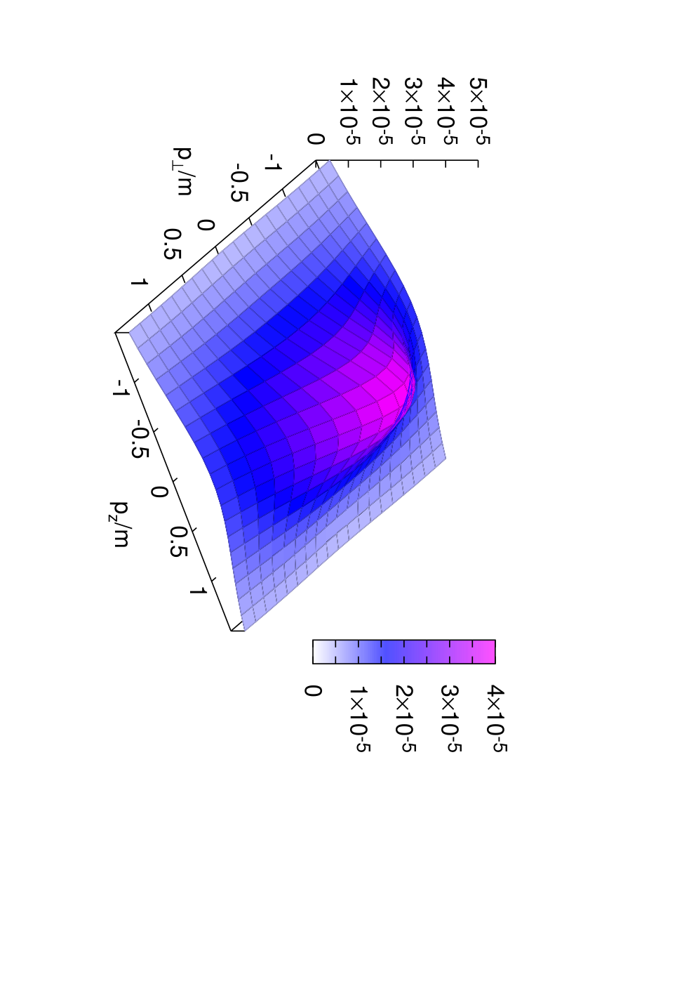
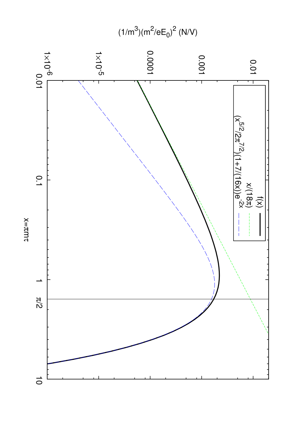
Figure 1 shows the momentum ($p$) dependence of the electron number density $(1/V)d^{3}N/d\mbox{\boldmath$p$}^{3}$ (18) for $|eE_{0}|/m^{2}=10$ and $m\tau=0.01$. We see that the peak is located at $\mbox{\boldmath$p$}={\bf 0}$, which reflects the fact that the energy threshold for creating one $e^{+}e^{-}$ pair ${\mathcal{E}}_{\rm thres}=2p_{0}$ takes its minimum ${\mathcal{E}}_{\rm thres}=2m$ at $\mbox{\boldmath$p$}={\bf 0}$. We also find that the distribution decays exponentially for large $p_{\perp}$. Actually, one can check this by taking the limit of $p_{\perp}\gg p_{z},m$:

$\displaystyle\frac{1}{V}\frac{d^{3}N}{d\mbox{\boldmath$p$}^{3}}\overset{p_{\perp}\gg p_{z},m}{\longrightarrow}\frac{1}{2\pi}\left|\frac{eE_{0}}{m^{2}}\right|^{2}(m\tau)^{4}{\rm e}^{-2\pi|\mbox{\boldmath{\small$p$}}_{\perp}|\tau}.$

(24)

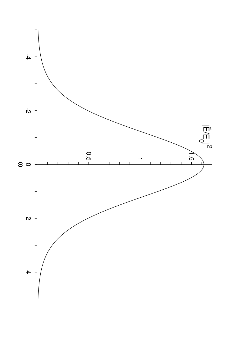
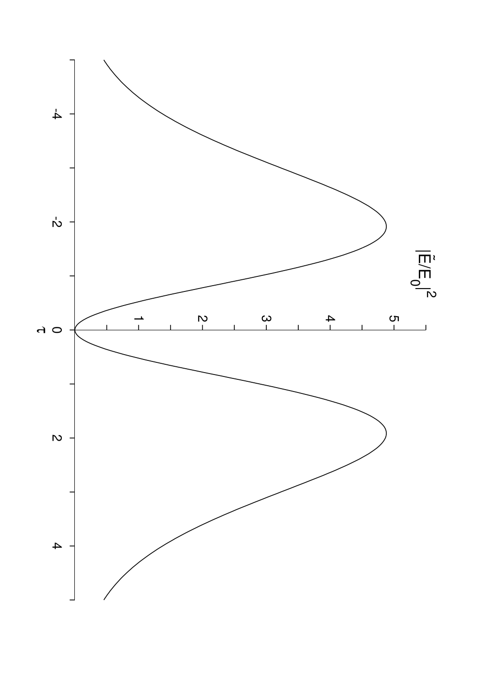
Figure 2 shows the $\tau$ dependence of the total electron number $N/V$. As is seen in Fig. 2, $N$ increases monotonically for small $m\tau$ while it decreases exponentially for large $m\tau$. This tendency can be roughly understood as follows: Since the threshold energy of the pair creation is ${\mathcal{E}}_{\rm thres}\sim 2m$, the background field must supply energy $\Omega$ larger than $2m$ for the pair creation to occur. In our computation based on the lowest-order perturbation theory, such energy $\Omega$ is supplied by a single (virtual) photon from the background electric field $E$. Since the typical energy $\omega$ of a photon which forms the Sauter-type background field $E$ is $\omega\sim 1/\tau$ (see Eq. (17) and the left panel of Fig. 3), we find $\Omega\sim$ (number of photons) $\times$ (typical photon energy) $\sim 1\times\omega\sim 1/\tau$. Thus, $\Omega\gtrsim 2m$ i.e., $m\tau\lesssim 1/2$ is required for the pair creation in the lowest order perturbation theory. The upper limit $m\tau=1/2$ is shown as a vertical line in Fig. 2. Pair creation from a single photon occurs when the pulse duration $\tau$ is short enough. On the other hand, as shown in the right panel of Fig. 3, the strength of the Fourier component $\tilde{E}(\omega)$ decreases with decreasing $\tau$. This essentially explains the decrease of electron number density for $\tau\to 0$ as seen in Fig. 2.

One can obtain analytic solutions to the Dirac equation in the presence of the Sauter-type background field [14, 12, 13] (see also Ref. [9] for discussion in $SU(2)$ case), which enables us to compute the number of produced electrons (15). After some calculations, one finds

$\displaystyle\frac{(2\pi)^{3}}{V}\frac{d^{3}N}{d\mbox{\boldmath$p$}^{3}}$

$\displaystyle=\frac{\sinh\left[\frac{\pi\tau}{2}\left(2eE_{0}\tau+p_{0}^{(-)}-p_{0}^{(+)}\right)\right]\sinh\left[\frac{\pi\tau}{2}\left(2eE_{0}\tau-p_{0}^{(-)}+p_{0}^{(+)}\right)\right]}{\sinh\left[\pi\tau p_{0}^{(-)}\right]\sinh\left[\pi\tau p_{0}^{(+)}\right]}\,,$

(25)

where $p_{0}^{(\pm)}\equiv\sqrt{m^{2}+\mbox{\boldmath$p$}_{\perp}^{2}+(p_{z}\pm eE_{0}\tau)^{2}}$ are the energy of the electron (positron) with the transverse momentum $\mbox{\boldmath$p$}_{\perp}$ and the canonical longitudinal momentum $p_{z}$. Note that the corresponding electron mode originally has the kinetic longitudinal momentum $p_{z}-eE_{0}\tau$ in the infinite past and $p_{z}+eE_{0}\tau$ in the infinite future. We stress that this result is clearly nonperturbative with respect to the coupling constant $e$, while the lowest order perturbation gave the result proportional to $e^{2}$ [see Eq. (18)]. The total number of produced electrons, $N/V$, is obtained after integration over the momentum $p$.

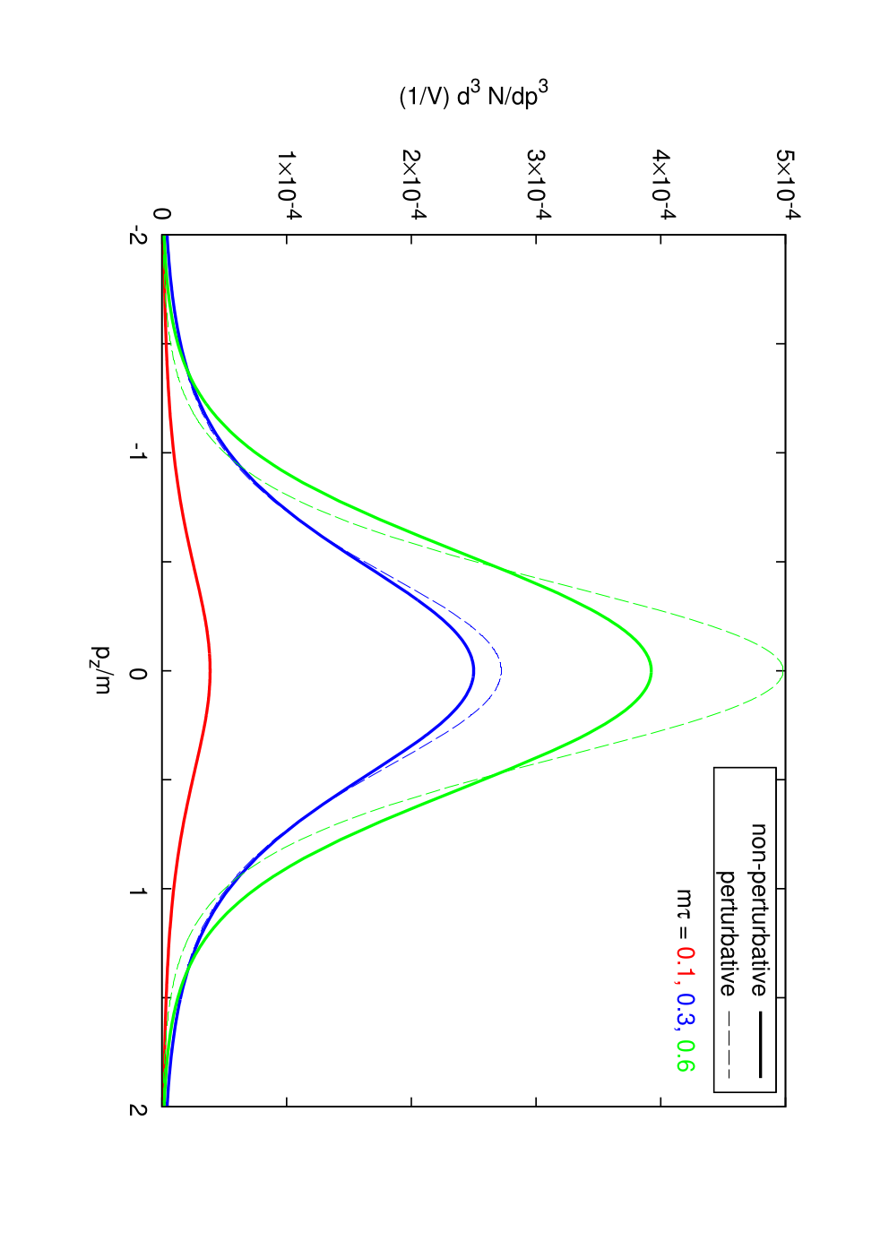
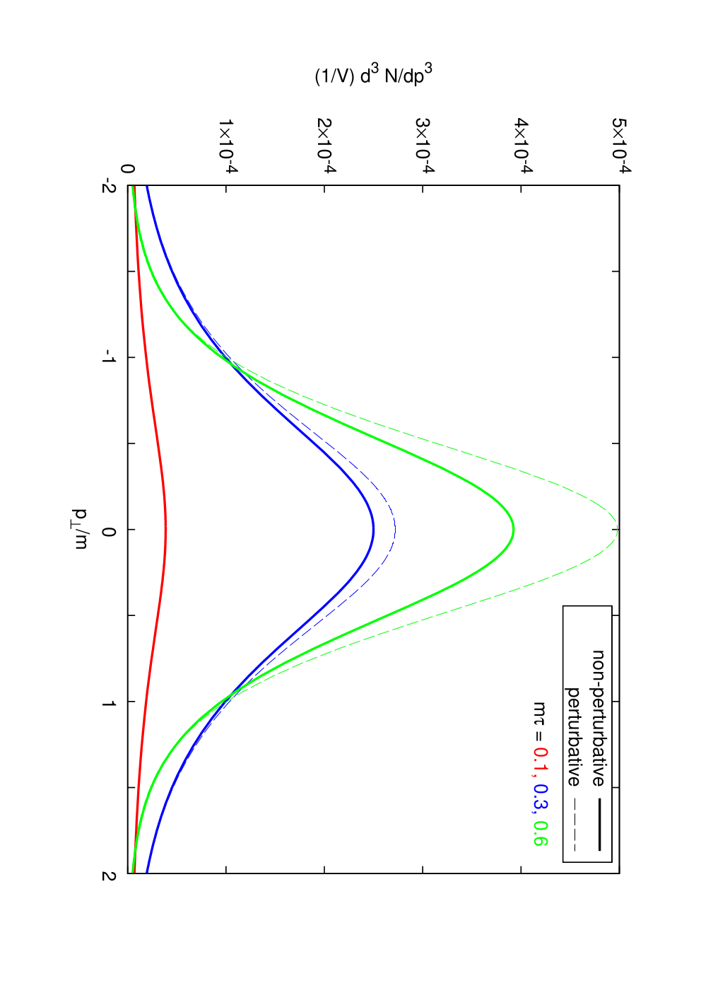
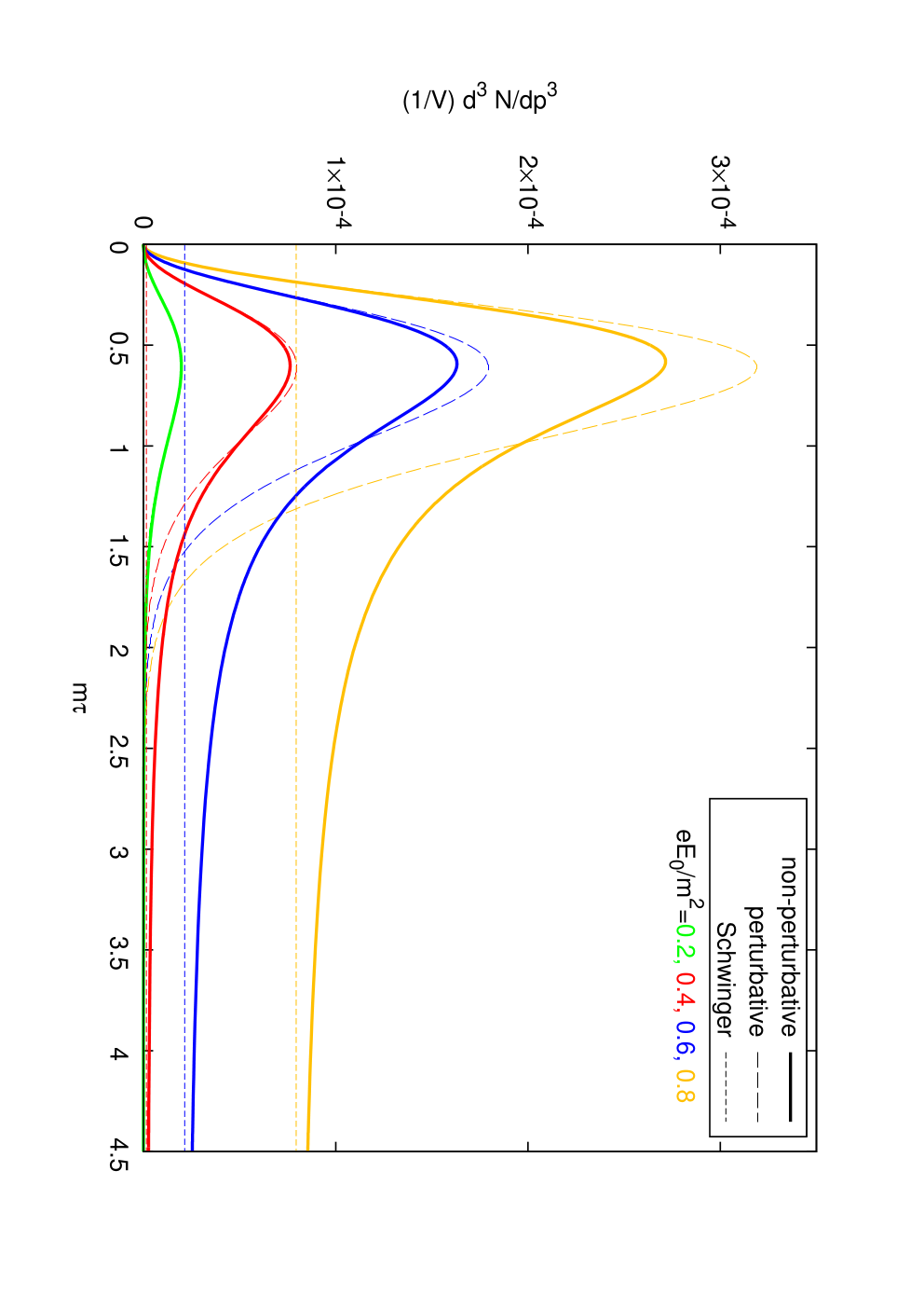
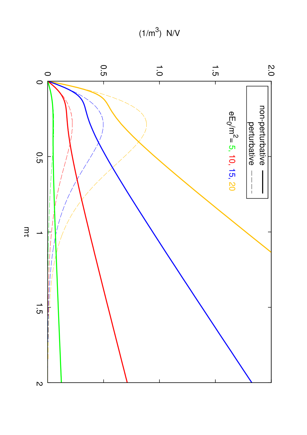
We compare the nonperturbative result (25) with the perturbative one (18) and (19) in Figs. 4, 5, and 6. Figure 4 shows the comparison of the momentum ($p_{z}$, $p_{\perp}$) dependence of the number density of electrons $d^{3}N/d\mbox{\boldmath$p$}^{3}$. The peak strength of the field is taken as $|eE_{0}|/m^{2}=1$. Three lines are for different values of $\tau$. We have shown only relatively short pulse cases: $m\tau=0.1,\,0.3,$ and 0.6. We immediately observe that the nonperturbative result (25) and the perturbative result (18) coincide with each other for the short pulse. The deviation becomes larger as $\tau$ increases, which can be explicitly seen in Fig. 5. There, $\tau$ dependence is shown for different values of the peak strength: The left panel is for the subcritical^†† † We tentatively use the words “supercritical” and “subcritical” for the cases $|eE_{0}|/m^{2}>1$ and $|eE_{0}|/m^{2}<1$, respectively, but precisely speaking, the condition $|eE_{0}|/m^{2}=1$ (valid for a constant electric field) does not play the same role for finite pulses. field strength $|eE_{0}|/m^{2}=0.2,\,0.4,\,0.6$ and 0.8 and the right panel is for the supercritical field strength $|eE_{0}|/m^{2}=5,\,10,\,15$ and 20. We again observe the agreement of the two results for short pulses $m\tau\ll 1$ no matter how large the field strength $|eE_{0}|/m^{2}$ is. However, the size of the agreement region in $\tau$ heavily depends on the field strength $|eE_{0}|/m^{2}$. For subcritical field strength $|eE_{0}|/m^{2}\lesssim 1$, perturbative result dominates the nonperturbative result even when the pulse is not very short $m\tau\sim 1$. On the other hand, for supercritical field strength $|eE_{0}|/m^{2}\gtrsim 1$, perturbative description is applicable only for very short pulse region $m\tau\ll 1$. We will clarify the reason for this behavior in the later discussion. The important point here is that for any field strength $|eE_{0}|/m^{2}$ there surely exists a region (short pulse region) where pair creation can be understood as a purely perturbative phenomenon. We can also observe that there is a clear deviation between the two in the long pulse region where the nonperturbative result approaches Schwinger’s result (horizontal lines). In particular, the deviation is larger for supercritical field $|eE_{0}|/m^{2}\gtrsim 1$. This can be understood as follows. Notice first that the perturbative result always approaches 0 in the long pulse limit $m\tau\gg 1$ because the typical energies of a (virtual) photon which forms the Sauter-type field $\omega\sim 1/\tau\rightarrow 0$ for large $\tau$ and thus not enough to create a pair. On the other hand, Schwinger’s formula valid in the long pulse region says that pair creation for subcritical field strength is exponentially suppressed $d^{3}N/d\mbox{\boldmath$p$}^{3}\propto\exp\{-\pi m^{2}/|eE_{0}|\}$. Therefore, the deviation between the two is almost negligible for weak field strength $|eE_{0}|/m^{2}\lesssim 1$, while it increases with increasing peak strength $|eE_{0}|/m^{2}$ in the supercritical regime $|eE_{0}|/m^{2}\gtrsim 1$.

The same tendency is found in the comparison of the total number of electrons $N$ as shown in Fig. 6. We note that the peak structure in the short pulse region is reproduced by the perturbative result quite well. Although for small $p_{z}$ the perturbative value of the density $d^{3}N/d\mbox{\boldmath$p$}^{3}$ is somewhat larger than the nonperturbative one, while it becomes smaller for large $p_{z}$ (see the left panel of Fig. 4), these differences cancel out with each other in integration over $p_{z}$. Thus we have a nice agreement in the total number $N$ as displayed in Fig. 6.

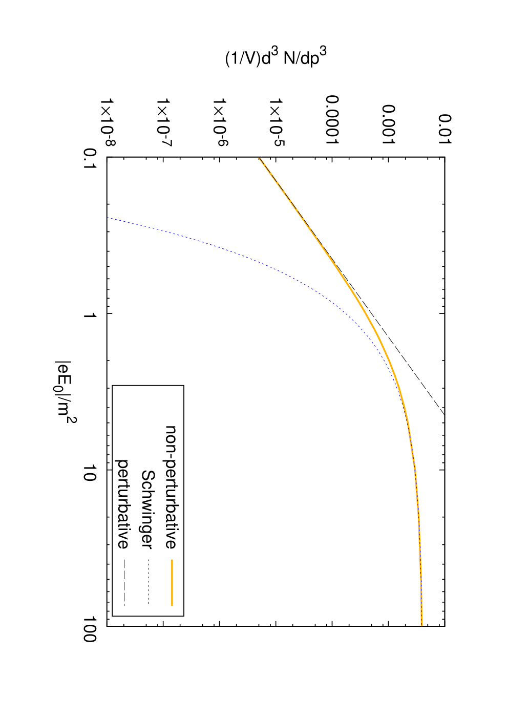
Figure 5 also shows an interesting behavior. For relatively short pulses $m\tau\lesssim 1$ with subcritical field strength $|eE_{0}|/m^{2}\lesssim 1$ (left panel), the results of the Sauter-type field are enhanced as compared to Schwinger’s value (horizontal lines). Since the pair creation in this region is dominated by the perturbative contribution, this enhancement should be understood as a purely perturbative effect. It shows up because Schwinger’s nonperturbative result $d^{3}N/d\mbox{\boldmath$p$}^{3}\propto\exp\{-\pi m^{2}/|eE_{0}|\}$ is exponentially small for subcritical field strength $|eE_{0}|/m^{2}\lesssim 1$, while the perturbative result is only power-suppressed as $d^{3}N/d\mbox{\boldmath$p$}^{3}\propto|eE_{0}/m^{2}|^{2}$ (see Eq. (5)). By using the perturbative formula for $d^{3}N/d\mbox{\boldmath$p$}^{3}$ (18), we immediately find that the peak position $\tau_{\rm peak}$ is given by $2=(\pi p_{0}\tau_{\rm peak})\coth[\pi p_{0}\tau_{\rm peak}]$ or $p_{0}\tau_{\rm peak}\sim 0.61$, which does not depend on the field strength $|eE_{0}|$ as is seen in Fig. 5. Accordingly, the peak value is given by $(1/V)d^{3}N/d\mbox{\boldmath$p$}^{3}\sim(5.0\times 10^{-4})\times(1-p_{z}^{2}/p_{0}^{2})|eE_{0}/p^{2}_{0}|^{2}$.

The peak value, ${\rm max}_{\tau}\left[d^{3}N/d\mbox{\boldmath$p$}^{3}\right]$, at ${\boldsymbol{p}}={\bf 0}$ is displayed in Fig. 7 as a function of the field strength $|eE_{0}|/m^{2}$, together with Schwinger’s value and the peak value of the perturbative contribution. The extrapolation of Schwinger’s value to the weak field case $|eE_{0}|/m^{2}\lesssim 1$ underestimates the pair creation in the Sauter-type pulsed field; the pair creation from the vacuum in the region $|eE_{0}|/m^{2}\lesssim 1,m\tau\lesssim 1$ is actually more abundant than Schwinger’s value, owing to the perturbative contribution with a single photon. Indeed, the compact formula for the perturbative peak nicely describes the enhancement for the subcritical fields, which is explicitly depicted with a dashed line in Fig. 7. Similar behavior was found in Refs. [9, 10], who however regarded this peak as a result of nonperturbative physics.

Now we return to the question: To what extent are we able to say a pulse is short? To answer this, we expand the nonperturbative result (25) by the pulse duration $\tau$. More precisely, we expand (25) by the following two dimensionless parameters,

	$\displaystyle\nu\equiv|eE_{0}|\tau^{2}\,,$		(26)
	$\displaystyle\gamma\equiv\frac{|eE_{0}|\tau}{m}\,,$		(27)

because there are two dimensionful quantities $|eE_{0}|,\,m$ in addition to $\tau$. The result is

	$\displaystyle{\rm Eq.(\ref{eqa16})}\!$	$\displaystyle=\!\frac{\!\sinh\!\!\left[\pi\nu\!\left(1\!+\!\frac{1}{2\gamma}\!\sqrt{\gamma^{2}\!-\!2\frac{p_{z}}{p_{0}}\gamma\!+\!1}\!-\!\frac{1}{2\gamma}\!\sqrt{\gamma^{2}\!+\!2\frac{p_{z}}{p_{0}}\gamma\!+\!1}\right)\!\right]\!\sinh\!\!\left[\pi\nu\!\left(1\!-\!\frac{1}{2\gamma}\!\sqrt{\gamma^{2}\!-\!2\frac{p_{z}}{p_{0}}\gamma\!+\!1}\!+\!\frac{1}{2\gamma}\!\sqrt{\gamma^{2}\!+\!2\frac{p_{z}}{p_{0}}\gamma\!+\!1}\right)\!\right]\!}{\sinh\left[\pi\nu\sqrt{1-2\frac{p_{z}}{p_{0}}\gamma^{-1}+\gamma^{-2}}\right]\sinh\left[\pi\nu\sqrt{1+2\frac{p_{z}}{p_{0}}\gamma^{-1}+\gamma^{-2}}\right]}$
		$\displaystyle\longrightarrow\left\{\begin{array}[]{ll}\displaystyle\frac{1}{(2\pi)^{3}}\left(1-\frac{p_{z}^{2}}{p_{0}^{2}}\right)\left|\frac{eE_{0}}{p^{2}_{0}}\right|^{2}\frac{(\pi p_{0}\tau)^{4}}{\pi^{2}\left|{\rm sinh}[\pi p_{0}\tau]\right|^{2}}&\quad(\nu,\gamma\ll 1)\\ \displaystyle{\rm exp}\left[-\frac{\pi\left(m^{2}+\mbox{\boldmath$p$}^{2}_{\perp}\right)}{|eE_{0}|}\right]&\quad(\nu,\gamma\gg 1)\,.\end{array}\right.$

Notice that the asymptotic forms (3.3) exactly reproduce the perturbative result (18) for $\nu,\gamma\ll 1$ and the nonperturbative expression for the Schwinger mechanism in a constant electric background field [5] for $\nu,\gamma\gg 1$. Thus, we conclude that pulses, such that the condition $\nu,\gamma\ll 1$ i.e., $m\tau\ll\sqrt{m^{2}/|eE_{0}|},m^{2}/|eE_{0}|$ is satisfied, are so short that pair creation becomes purely perturbative, where the lowest order perturbation theory works very nicely. On the other hand, pulses, such that the condition $\nu,\gamma\gg 1$ i.e., $m\tau\gg\sqrt{m^{2}/|eE_{0}|},m^{2}/|eE_{0}|$ is satisfied, are so long that pair creation becomes nonperturbative, where perturbation theory completely breaks down. We can also say that for middle pulses, such that neither condition $\nu,\gamma\gg 1$ nor $\nu,\gamma\ll 1$ is satisfied, perturbation theory is still applicable; however, the lowest-order perturbation theory does not work because higher-order corrections ${\mathcal{O}}((eE)^{n})$ ($n>1$) become important. We summarize our picture in Fig. 8. These considerations clearly show that in order to investigate the nonperturbative nature of the Schwinger mechanism we must require not only the strength $|eE_{0}|/m^{2}\gtrsim 1$ but also a sufficient duration $m\tau\gg\sqrt{m^{2}/|eE_{0}|},m^{2}/|eE_{0}|$; otherwise pair creation from the vacuum can be understood simply as a perturbative phenomenon.

The discussion given above is a natural result if we consider the meaning of the dimensionless parameters $\nu,\,\gamma$. Recall the fact that the work $W$ done by a pulsed electric background field with height $E_{0}$ and width $\tau$ is given by $W\sim|eE_{0}|\tau$ and that the typical energy $\omega$ of a photon that forms the pulsed background field is given by $\omega\sim 1/\tau$. Then, we can understand the physical meaning of $\nu,\,\gamma$ as follows: $\nu\sim W/\omega$ is the number of (virtual) photons of the background field involved in a scattering process. $\gamma\sim W/m\sim\nu\omega/m$ is the work done by the background field scaled by the typical energy scale of the system $m$. Keeping these in mind, we can interpret that the perturbative condition $\nu,\gamma\ll 1$ corresponds to the case where both the number of photons involved in a scattering process $\nu$ and its correction to the system $\gamma$ are very small. This is obviously a natural criterion for the lowest order perturbation theory to work. We can also interpret the nonperturbative condition $\nu,\gamma\gg 1$ in the same way.

It is interesting to compare our discussion with Ref. [15], which claims that the Keldysh parameter $\gamma_{\rm K}=|eE|/(m\omega)$, where $\omega$ is the typical frequency of the background field, discriminates whether the system is perturbative or nonperturbative. Note that their discussion is limited to the case where (i) an oscillating electric field background $E(t)=E_{0}\cos\omega t$, (ii) $\omega$ is sufficiently small compared to the electron mass $\omega/m\ll 1$, and (iii) the background field is sufficiently weak $|eE_{0}|/m^{2}\ll 1$. If we assume that the typical frequency $\omega$ of a pulsed background field is given by the inverse of the pulse duration $\omega\sim 1/\tau$, we find that our discussion obtained in a pulsed background field (see Fig. 8) agrees with Ref. [15] as long as the limitation (iii) is satisfied. In such a condition, $\gamma$ determines the “perturbativeness” of the system in our discussion and is equivalent to the Keldysh parameter because $\gamma=\frac{|eE_{0}|}{m(1/\tau)}\sim|eE_{0}|/(m\omega)=\gamma_{\rm K}$.

REFERENCES

- [1] The diversity of strong-field physics can be seen in the proceedings and web pages of a series of workshops, Physics in Intense Fields (PIF): PIF2010, November 2010, KEK, Japan, edited by K.Itakura, et al., http://ccdb5fs.kek.jp/tiff/2010/1025/1025013.pdf and http://atfweb.kek.jp/pif2010/; PIF2013, July 2013, DESY Hamburg, https://indico.desy.de/conferenceDisplay.py?confId=7155.
- [2] For a review, see for example, W. Greiner, B. Muller and J. Rafelski, Quantum Electrodynamics of Strong Fields, Texts and Monographs in Physics (Springer, Berlin, 1985).
- [3] F. Sauter, Z. Phys. 69, 742 (1931).
- [4] W. Heisenberg and H. Euler, Z. Phys. 98, 714, (1936); English translation is available from arXiv: physics/0605038.
- [5] J. Schwinger, Phys. Rev. 82, 664 (1951).
- [6] G. V. Dunne, arXiv:hep-th/0406216.
- [7] F. Hebenstreit, R. Alkofer, and H. Gies, Phys. Rev. D 78, 061701 (2008).
- [8] C. Kohlfurst, M. Mitter, G. von Winckel, F. Hebenstreit, and R. Alkofer, Phys. Rev. D 88, 045028 (2013).
- [9] P. Levai and V. Skokov, Phys. Rev. D 82, 074014 (2010).
- [10] V.V. Skokov and P. Levai, Phys. Rev. D 78, 054004 (2008).
- [11] A.I. Nikishov, Sov. Phys. JTEP 30, 660 (1970).
- [12] N.B. Narozhnyi, A.I. Nikishov, Yad. Fiz. 11, 1072 (1970) [Sov. J. Nucl. Phys. 11, 596 (1970)].
- [13] F. Hebenstreit, Ph.D. thesis, Karl-Franzens-Universität, 2011, arXiv:1106.5965 [hep-ph].
- [14] F. Sauter, Z. Phys. 73, 547 (1932).
- [15] E. Brezin and C. Itzykson, Phys. Rev. D 2, 1191 (1970).
- [16] A. Bzdak and V. Skokov, Phys. Lett. B 710, 171 (2012).
- [17] W.T. Deng and X.G. Huang, Phys. Rev. C 85, 044907 (2012).