Empirical Bayes Estimation for the Stochastic Blockmodel
Abstract
Inference for the stochastic blockmodel is currently of burgeoning interest in the statistical community, as well as in various application domains as diverse as social networks, citation networks, brain connectivity networks (connectomics), etc. Recent theoretical developments have shown that spectral embedding of graphs yields tractable distributional results; in particular, a random dot product latent position graph formulation of the stochastic blockmodel informs a mixture of normal distributions for the adjacency spectral embedding. We employ this new theory to provide an empirical Bayes methodology for estimation of block memberships of vertices in a random graph drawn from the stochastic blockmodel, and demonstrate its practical utility. The posterior inference is conducted using a Metropolis-within-Gibbs algorithm. The theory and methods are illustrated through Monte Carlo simulation studies, both within the stochastic blockmodel and beyond, and experimental results on a Wikipedia graph are presented.
1 Introduction
The stochastic blockmodel (SBM) is a generative model for network data introduced in Holland et al. (1983). The SBM is a member of the general class of latent position random graph models introduced in Hoff et al. (2002). These models have been used in various application domains as diverse as social networks (vertices may represent people with edges indicating social interaction), citation networks (who cites whom), connectomics (brain connectivity networks; vertices may represent neurons with edges indicating axon-synapse-dendrite connections, or vertices may represent brain regions with edges indicating connectivity between regions), and many others. For comprehensive reviews of statistical models and applications, see Fienberg (2010), Goldenberg et al. (2010), Fienberg (2012). In general, statistical inference on graphs is becoming essential in many areas of science, engineering, and business.
The SBM supposes that each of vertices is assigned to one of blocks. The probability of an edge between two vertices depends only on their respective block memberships, and the presence of edges are conditionally independent given block memberships. By letting denote the block to which vertex i is assigned, a matrix is defined as the probability matrix such that the entry is the probability of an edge between vertices and . The block proportions are represented by a -dimensional probability vector . Given an SBM graph, estimating the block memberships of vertices is an obvious and important task. Many approaches have been developed for estimation of vertex block memberships, including likelihood maximization (Bickel and Chen, 2009, Choi et al., 2012, Celisse et al., 2012, Bickel et al., 2013), maximization of modularity (Newman, 2006), spectral techniques (Rohe et al., 2011, Sussman et al., 2012, Fishkind et al., 2013), and Bayesian methods (Snijders and Nowicki, 1997, Nowicki and Snijders, 2001, Handcock et al., 2007, Airoldi et al., 2008).
Latent position models for random graphs provide a framework in which graph structure is parametrized by a latent vector associated with each vertex. In particular, this paper considers the special case of the latent position model known as the random dot product graph model (RDPG), introduced in Nickel (2006) and Young and Scheinerman (2007). In the RDPG, each vertex is associated with a latent vector, and the presence or absence of edges are independent Bernoulli random variables, conditional on these latent vectors. The probability of an edge between two vertices is given by the dot product of the corresponding latent vectors. An SBM can be defined in terms of an RDPG model for which all vertices that belong to the same block share a common latent vector.
When analyzing RDPGs, the first step is often to estimate the latent positions, and these estimated latent positions can then be used for subsequent analysis. Obtaining accurate estimates of the latent positions will consequently give rise to accurate inference (Sussman et al., 2014), as the latent vectors determine the distribution of the random graph.
Sussman et al. (2012) describes a method for estimating the latent positions in an RDPG using a truncated eigen-decomposition of the adjacency matrix.
Athreya et al. (2015) proves that for an RDPG, the latent positions estimated using adjacency spectral graph embedding converge in distribution to a multivariate Gaussian mixture. This suggests that we may consider the estimated latent positions of a -block SBM as (approximately) an independent and identically distributed sample from a mixture of multivariate Gaussians.
In this paper, we demonstrate the utility of an estimate of this multivariate Gaussian mixture as an empirical prior distribution in a Bayesian inference methodology for estimating block memberships in an SBM graph, as it quantifies residual uncertainty in the model parameters after adjacency spectral embedding.
This paper is organized as follows. In Section 2, we formally present the SBM as an RDPG model and describe how the theorem of Athreya et al. (2015) motivates our mixture of Gaussians empirical prior. We then present our empirical Bayes methodology for estimating block memberships in the SBM, and the Markov chain Monte Carlo (MCMC) algorithm that implements the Bayesian solution. In Section 4, we present simulation studies and an experimental analysis demonstrating the performance of our empirical Bayes methodology. Finally, Section 5 discusses further extensions and provides a concluding summary.
2 Background
Network data on vertices may be represented as an adjacency matrix . We consider simple graphs, so that is symmetric (undirected edges imply for all ), hollow (no self-loops implies for all ), and binary (no multi-edges or weights implies for all ). For our random graphs, the vertex set is fixed; it is the edge set that is random.
Let be a set such that implies ,
let on ,
and write .
Definition 1 (Random Dot Product Graph).
A random graph with adjacency matrix is said to be a random dot product graph (RDPG) if
Thus, in the RDPG model, each vertex is associated with a latent vector . Furthermore, conditioned on the latent positions , the edges .
For an RDPG, we also define the edge probability matrix ; is symmetric and positive semidefinite and has rank at most . Hence, has a spectral decomposition given by where , and has orthonormal columns, and is diagonal matrix with non-negative non-increasing entries along the diagonal. It follows that there exists an orthonormal such that . This introduces obvious non-identifiability since generates the same distribution over adjacency matrices (i.e. ). As such, without loss of generality, we consider uncentered principal components (UPCA) of , , such that . Letting and be the adjacency matrix versions of and , the adjacency spectral graph embedding (ASGE) of to dimension is given by .
The SBM can be formally defined as an RDPG for which all vertices that belong to the same block share a common latent vector, according to the following definition.
Definition 2 ((Positive Semidefinite) Stochastic Blockmodel).
An RDPG can be parameterized as an SBM with blocks if the number of distinct rows in is . That is, let the probability mass function associated with the distribution of the latent positions be given by the mixture of point masses , where the probability vector satisfies and the distinct latent positions are represented by . Thus the standard definition of the SBM with parameters and is seen to be an RDPG with .
Additionally, for identifiability purposes, we impose the constraint that the block probability matrix have distinct rows; that is, for all .
In this setting, the block memberships Discrete such that if and only if . Let be the number of vertices such that ; we will condition on throughout. Given a graph generated according to the SBM, our goal is to assign vertices to their correct blocks.
To date, Bayesian approaches for estimating block memberships in the SBM have typically involved a specification of the prior on the block probability matrix ; the beta distribution (which includes the uniform distribution as a special case) is often chosen as the prior (Snijders and Nowicki, 1997, Nowicki and Snijders, 2001). Facilitated by our re-casting of the SBM as an RDPG and motivated by recent theoretical advances described in Section 3.1 below, we will instead derive an empirical prior for the latent positions themselves.
3 Model
This section presents the models and algorithms we will use to investigate the utility of the empirical Bayes methodology for estimating block memberships in an SBM graph as detailed in Section 3.1 and referred to as ASGE.
For comparison purposes, in Sections 3.2 and 3.3 we construct an alternative Flat and two benchmark models, as outlined below. Note that all four models are named after their respective prior distributions used for the latent positions .
- •
Flat – an alternative to the proposed empirical Bayes prior distribution for . Since in the absence of the ASGE theory a natural choice for the prior on is the uniform distribution on the parameter space.
- •
Exact – a primary benchmark model where all model parameters, except the block membership vector , are assumed known.
- •
Gold – a secondary benchmark model where and are the unknown parameters; the gold standard mixture of Gaussians prior distribution for takes its hyperparameters to be the true latent positions and theoretical limiting covariances motivated by the distributional results from Athreya et al. (2015) presented in Section 3.1.
3.1 The Empirical Bayes with ASGE Prior Model (“ASGE”)
Recently, Athreya et al. (2015) proved that for an RDPG
the latent positions estimated using adjacency spectral graph embedding converge in distribution to a multivariate Gaussian mixture.
We can express this more formally in a central limit theorem (CLT) for the scaled differences between the estimated and true latent positions of the RDPG graph, as well as a corollary to motivate our empirical Bayes prior (henceforth denoted ASGE).
Theorem 3 (Athreya et al. (2015)).
Let be an RDPG with -dimensional latent positions , and assume distinct eigenvalues for the second moment matrix of . Let be the UPCA of so that the columns of are orthogonal, and let be the estimate for . Let represent the cumulative distribution function for the multivariate normal, with mean and covariance matrix . Then for each row of and of ,
where the integral denotes a mixture of the covariance matrices and, with the second moment matrix ,
The special case of the SBM gives rise to the following corollary.
Corollary 4.
Note that the distribution of the latent positions remains unchanged, as .
This gives rise to the mixture of normals approximation for the estimated latent positions obtained from the adjacency spectral embedding. That is, based on these recent theoretical results, we can consider the estimated latent positions as (approximately) an independent and identically distributed sample from a mixture of multivariate Gaussians.
A similar Bayesian method for latent position clustering of network data is proposed in Handcock et al. (2007). Their latent position cluster model is an extension of Hoff et al. (2002), wherein all the key features of network data are incorporated simultaneously – namely clustering, transitivity (the probability that the adjacent vertices of a vertex having a connection), and homophily on attributes (the tendency of vertices with similar features to possess a higher probability of presenting an edge). The latent position cluster model is similar to our model, but they use the logistic function instead of the dot product as their link function.
Our theory gives rise to a method for obtaining an empirical prior for using the adjacency spectral embedding. Given the estimated latent positions obtained via the spectral embedding of the adjacency matrix , the next step is to cluster these using Gaussian mixture models (GMM). There are a wealth of methods available for this task; we employ the model-based clustering of Fraley and Raftery (2002) via the R package MCLUST which implements an Expectation-Maximization (EM) algorithm for maximum likelihood parameter estimation. This mixture estimate, in the context of Corollary 4, quantifies our uncertainty about , suggesting its role as an empirical Bayes prior distribution. That is, our empirical Bayes prior distribution for is expressed as
| (2) |
where is the density function of a multivariate normal distribution with mean and covariance matrix denoting standard maximum likelihood estimates (via Expectation-Maximization algorithm) based on the estimated latent positions and the indicator enforces homophily and block identifiability constraints for the SBM via
Algorithm 1 provides steps for obtaining the empirical Bayes prior using the ASGE and GMM.
In the setting of Corollary 4, for an adjacency matrix , the likelihood for the block membership vector and the latent positions is given by
| (3) |
This is the case where the block memberships , the latent positions , and the block membership probabilities are assumed unknown. Thus, our empirical posterior distribution for the unknown quantities is given by
where a multinomial distribution is posited as a prior distribution on with the hyperparameter , chosen to follow a Dirichlet distribution with parameters for all in the unit simplex , and a multivariate normal prior on as expressed in Eqn 2. To summarize, the prior distributions on the unknown quantities , , and are
By choosing a conjugate Dirichlet prior for , we can marginalize the posterior distribution over as follows:
Let denote the block assignment counts, where . Then the resulting prior distribution is given by
which follows a Multinomial-Dirichlet distribution with parameters and . Therefore, the marginal posterior distribution can be expressed as
We can sample from the marginal posterior distribution for and via Metropolis–Hasting–within–Gibbs sampling. A standard Gibbs sampling update is employed to sample the posterior of , which can be updated sequentially. The idea behind this method is to first posit a full conditional posterior distribution of . Let denote the block memberships for all but vertex . Then, conditioning on , we have
| (4) |
Hence, the posterior distribution for where
| (5) |
The procedure consists of visiting each for and executing Algorithm 2. We initialize with , the block assignment vector obtained from GMM clustering of the estimated latent positions . For the Metropolis sampler for , the prior distribution as expressed in Eqn (2) will be employed as the proposal distribution. We generate a proposed state with the acceptance probability defined as
where in the denominator denotes the current state. The initialization of is .
for the block membership vector and the latent positions
3.2 The Alternative “Flat” Model
In the event that no special prior information is available, a natural choice of prior is the uniform distribution on the parameter space. This results in the formulation of the Flat model as an alternative to an empirical Bayes prior distribution for discussed in the previous section. We consider a flat prior distribution on the constraint set , where the marginal posterior distribution for and is given by
The Gibbs sampler for is identical to the procedure presented in Section 3.1. As for the Metropolis sampler for the latent positions , the flat prior distribution is used as the proposal. However, we initialize by generating it from the prior distribution of as ASGE, i.e. .
3.3 Comparison Benchmarks
“Exact”
This is our primary benchmark where the latent positions and the block membership probabilities are assumed known. Thus, the posterior distribution for the block memberships is given by
We can draw inferences about based on the posterior via an Exact Gibbs sampler using its full-conditional distribution,
| (6) |
which is the multinomial density where
| (7) |
Hence, for our Exact Gibbs sampler, once a vertex is selected, the exact calculation of and sample from the can easily be obtained. Initialization of will be .
“Gold”
For our secondary benchmark, we assume is known and that both and are unknown. Here we describe what we call the Gold standard prior distribution.
Let the true value for the latent positions be represented by . Based on Corollary 4, we can suppose that the prior distribution for follows a (truncated) multivariate Gaussian centered at and with covariance matrix given by the theoretical limiting distribution for the adjacency spectral embedding presented in Eqn (1) (i.e. ). This corresponds to the approximate distribution of if we condition on . This gold standard prior can be thought of as an oracle; however, in practice the theoretical and are not available.
Inference for and is based on the posterior distribution, , estimated by samples obtained from a Gibbs sampler for and an Independent Metropolis sampler for . Thus, the posterior distribution for the unknown quantities is given by
In this case, the Gibbs sampler for will be identical to that for Exact except the initial state will be given by , the block assignment vector obtained from GMM as explained in Section 3.1. Similar to the ASGE model, the prior distribution will be employed as the proposal distribution for the Metropolis sampler for .
Table 1 provides a summary of our Bayesian modeling schemes. The adjacency spectral graph embedding theory suggests that we might expect increasingly better performance as we go from Flat to ASGE to Gold to Exact. (As a teaser, we hint here that we will indeed see precisely this progression, in Section 4.)
| Models | Exact | Gold | ASGE | Flat | ||
|---|---|---|---|---|---|---|
| Parameters | ||||||
| Gibbs | Prior | |||||
| Initial Point | ||||||
| Independent Metropolis Hasting | Prior | |||||
| Initial point | ||||||
| Proposal | ||||||
4 Performance Comparisons
We illustrate the performance of our ASGE model via various Monte Carlo simulation experiments and one real data experiment. Specifically, we consider in Section 4.1 a SBM, in Section 4.2 a generalization of this SBM to a more general RDPG, in Section 4.3 a SBM, and in Section 4.4 a three-class Wikipedia graph example. We demonstrate the utility of the ASGE model for estimating vertex block assignments via comparison to competing methods.
Throughout our performance analysis, we generate posterior samples of and for a large number of iterations for two parallel Markov chains. The percentage of misassigned vertices per iteration is calculated and used to compute Gelman-Rubin statistics to check convergence of the chains. The posterior inference for is based on iterations after convergence. Performance is evaluated by calculating the vertex block assignment error. This procedure is repeated multiple times to obtain estimates of the error rates.
4.1 A Simulation Example with
Consider the SBM parameterized by
| (8) |
The block proportion vector indicates that each vertex will be in block 1 with probability and in block 2 with probability . Edge probabilities are determined by the entries of , independent and a function of only the vertex block memberships. This model can be parameterized as an RDPG in where the distribution of the latent positions is a mixture of point masses positioned at with prior probability 0.6 and with prior probability 0.4.
For each , we generate random graphs according to the SBM with parameters as provided in Eqn (8). For each graph , the spectral decomposition of the corresponding adjacency matrix provides the estimated latent positions .
Subsequently, GMM is used to cluster the embedded vertices, the result of which (estimated block memberships derived from the individual mixture component membership probabilities from the estimated Gaussian mixture model) is then reported as GMM performance as well as employed as the initial point in the Gibbs step for updating . The mixture component means and variances determine our empirical Bayes ASGE prior for the latent positions . The GMM estimate of block proportion vector in place of a conjugate Dirichlet prior on was considered, but no substantial performance improvements were realized. To avoid the model selection quagmire we assume and are known in this experiment.


Figure 1 presents a scatter plot of the estimated latent positions for one Monte Carlo replicate with . The colors denote the true block memberships for the corresponding vertices in the SBM. The symbols denote the cluster memberships given by the GMM. The ellipses represent the 95% level curves of the estimated GMM (black) and the theoretical GMM (green).

Results comparing with the alternative Flat, benchmark models, and GMM are presented in Figure 2. As expected, the error decreases for all models as the number of vertices increases. As previously explained in Section 3, Exact and Gold formulated in this study are perceived as benchmarks; it is expected that these models will show the best performance – for Exact, all the parameters are assumed known apart from the block memberships , while in the case of the Gold model, although the latent positions and are unknown parameters, their prior distributions were taken from the true latent positions and the theoretical limiting covariances.
The main message from Figure 2 is that our empirical Bayes model, ASGE, is vastly superior to that of both the alternative Flat model and GMM (the sign test -value for the paired Monte Carlo replicates is less than for both comparisons for all ) and nearly achieves Gold/Exact performance by . As an aside, we note that when we put a flat prior directly on , we obtain results indistinguishable from our Flat model on the latent positions.
A version of Theorem 3 for sparse random dot product graphs is given in Sussman (2014), and suggests an empirical Bayes prior for use in sparse graphs. A thorough investigation of comparative performance in this case is beyond the scope of this manuscript, but we have provided illustrative results in Figure 3 for the sparse graphs analogous to the setting presented in Eqn (8). For the same values of , we generate sparse random graphs from the following SBM:
For clarity, the plot includes only and GMM. Note that similar performance gains are obtained, with analogous ASGE superiority, in the sparse simulation setting (although absolute performance is of course degraded).

4.2 A Dirichlet Mixture RDPG Generalization
Here we generalize the simulation setting presented in Section 4.1 above to the case where the latent position vectors are distributed according to a mixture of Dirichlets as opposed to the SBM’s mixture of point masses. That is, we consider . Note that the SBM model presented in Section 4.1 is equivalent to the limit of this mixture of Dirichlets model as .
For , we report illustrative results using , for comparison with the SBM results from Section 4.1. Specifically, we obtain mean error rates of 0.4194, 0.2865, and 0.3705 for Flat, ASGE, and GMM, respectively; the corresponding results for the SBM, from Figure 2, are 0.3456, 0.2510, and 0.3910. Thus we see that, while the performance is slightly degraded, our empirical Bayes approach works well in this RDPG generalization of Section 4.1’s SBM. This demonstrates robustness of our method to violation of the SBM assumption.
4.3 A Simulation Example with
Our final simulation study considers the SBM parameterized by
| (9) |
In a same manner as Section 4.1, the model is parameterized as an RDPG in where the distribution of the latent positions is a mixture of point masses positioned at , , with equal probabilities. In this experiment, we assume that and are known.
Table 2 displays error rate estimates for this case, with and . In both cases, the ASGE model yields results vastly superior to the Flat model; e.g., for the mean error rate for Flat is approximately 11% compared to a mean error rate for ASGE of approximately 1%. Based on the paired samples, the sign test -value is less than for both values of . While the results of GMM appear competitive to the results of our empirical Bayes with ASGE prior in terms of mean and median error rate, the paired analysis shows again that the ASGE prior is superior, as seen by sign test -values < for both values of .
From Table 2, we see that for , empirical Bayes with ASGE prior has a mean error rate of percent (3 errors per graph) and a median error rate of 1/3 percent (1 error per graph), while GMM has a mean and median error rate of 1 percent. As an illustration, Figure 4 presents the histogram of the differential number of errors made by the ASGE model and GMM for . The histogram shows that for most graphs, empirical Bayes with ASGE prior performs as well as or better than GMM. (NB: In the histogram presented in Figure 4, eight ouliers in which ASGE performed particularly poorly are censored at a value of 10; we believe these outliers are due to chain convergence issues.
| (Flat) | mean | 0.3288 | 0.1137 |
|---|---|---|---|
| 95% CI | [0.3207,0.3369] | [0.1004,0.1270] | |
| median | 0.3600 | 0.0133 | |
| (ASGE) | mean | 0.1359 | 0.0107 |
| 95% CI | [0.1277,0.1440] | [0.0069,0.0145] | |
| median | 0.0733 | 0.0033 | |
| (GMM) | mean | 0.1438 | 0.0110 |
| 95% CI | [0.1396,0.1480] | [0.0104,0.0116] | |
| median | 0.1267 | 0.0100 |

4.4 Wiki Experiment
In this section we analyze an application of our methodology to the Wikipedia graph. The vertices of this graph represent Wikipedia article pages and there is an edge between two vertices if either of the associated pages hyperlinks to the other. The full data set consists of 1382 vertices – the induced subgraph generated from the two-hop neighborhood of the page “Algebraic Geometry.” Each vertex is categorized by hand into one of six classes – , , , , , and – based on the content of the associated article. (The adjacency matrix and the true class labels for this data set are available at http://www.cis.jhu.edu/~parky/Data/data.html.)
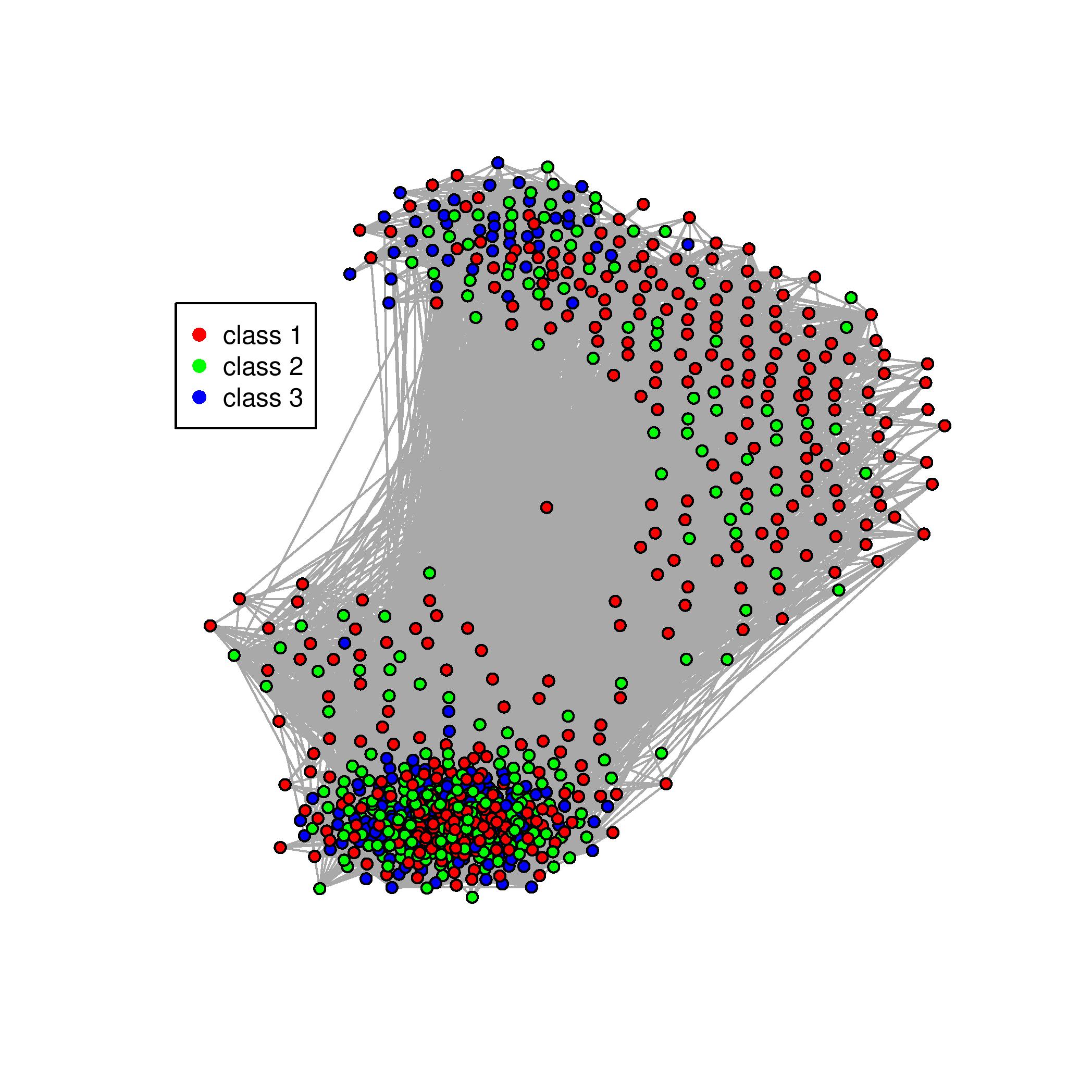
We analyze a subset of this data set corresponding to the classes , , and , labeled here as Class 1, 2 and 3, respectively. After excluding three isolated vertices in the induced subgraph generated by these three classes, we have a connected graph with a total of vertices; the class-conditional sample sizes are , , and . Figure 5 presents one rendering of this graph (obtained via one of the standard force-directed graph layout methods, using the command layout.drl in the igraph R package); Figure 6 presents the adjacency matrix; Figure 7 presents the pairs plot for the adjacency spectral embedding of this graph into . (In all figures, we use red for Class 1, green for Class 2 and blue for Class 3.) Figures 5, 6, and 7 indicate clearly that this Wikipedia graph is not a pristine SBM – real data will never be; nonetheless, we proceed undaunted.


We illustrate our empirical Bayes methodology, following Algorithm 1, via a bootstrap experiment. We generate bootstrap resamples from the adjacency spectral embedding depicted in Figure 7, with (). This yields for each bootstrap resample . It is important to note that we regenerate an RDPG based on the sampled latent positions, and proceed from this graph with our full empirical Bayes analysis, for each resample. This provides for valid inference conditional on the – that is, this bootstrap procedure is justified for confidence intervals assuming the true latent positions are , and provides for unconditional inference only asymptotically as .
As before, GMM is used to cluster the (embedded) vertices and obtain block label estimates and mixture component means and variances for each cluster of the estimated latent positions . The clustering result from GMM for one resample is presented in Figure 8. (We choose for the adjacency spectral embedding dimension because a common and reasonable choice is to use , which choice is justified in the SBM case (Fishkind et al., 2013).) The GMM clustering provides the empirical prior and starting point for our Metropolis–Hasting–within–Gibbs sampling (Algorithm 2) using the subgraph of the full Wikipedia graph induced by . (NB: For this Wikipedia experiment, the assumption of homophily is clearly violated; as a result, the constraint set used here is given by .)

Classification results for this experiment are depicted via boxplots in Figure 9. We see from the boxplots that using the adjacency spectral empirical prior does yield statistically significant improvement; indeed, our paired sample analysis yields sign test -values less than for both ASGE vs Flat and ASGE vs GMM. Notably, ASGE and Flat differ by in average, which is approximately 28 different classifications per graph. Despite similar predictions, ASGE improves Flat.
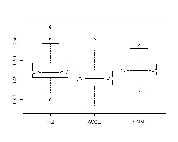
We have shown that using the empirical ASGE prior has improved performance compared to the Flat prior and GMM on this Wikipedia dataset. However, Figure 9 also indicates that ASGE performance on this data set, while representing a statistically significant improvement, might seem not very good in absolute terms: the mean probability of misclassification over bootstrap resamples is for ASGE versus for both Flat and GMM. That is, empirical Bayes using the adjacency spectral prior provides a statistically significant but perhaps unimpressive 2% improvement in the error rate. (Note that chance performance is .) Given that the Bayes optimal probability of misclassification is unknown, we consider where denotes the class of all classifiers based on class-conditional Gaussians. This yields an error rate of approximately . Note that this analysis assumes that a training set of labeled exemplars is available, which training information is not available in our empirical Bayes setting. Nonetheless, we see that our empirical Bayes methodology using the ASGE prior improves more than 25% of the way from the Flat and GMM performance to this (presumably unattainable) standard. As a final point, we note that a -nearest neighbor classifier (again, with a training set of labeled exemplars) yields an error rate of approximately , indicating that the assumption of class-conditional Gaussians was unwarranted. (Indeed, this is clear from Figure 7.) That our ASGE provides significant performance improvement despite the fact that our real Wikipedia data set so dramatically violates the stochastic block model assumptions is a convincing demonstration of the robustness of the methodology.
5 Conclusion
In this paper we have formulated an empirical Bayes estimation approach for block membership assignment. Our methodology is motivated by recent theoretical advances regarding the distribution of the adjaceny spectral embedding of random dot product and SBM graphs. To apply our model, we derived a Metropolis-within-Gibbs algorithm for block membership and latent position posterior inference.
Our simulation experiments demonstrate that the ASGE model consistently outperforms the GMM clustering used as our emprical prior as well as the alternative Flat prior model – notably, even in our Dirichlet mixture RDPG model wherein the SBM assumption is violated. For the Wikipedia graph, our ASGE model again performs admirably, even though this real data set is far from an SBM. Our results focus on demonstrating the utility of the Athreya et al. (2015) limit theorem for an SBM in providing an empirical Bayes prior as a mixture of Gaussians. Although there are myriad non-adjacency spectral embedding approaches, for ease of comparison we instead consider different Bayes samplers. One promising comparison for future investigation involves profile likelihood methods, which can potentially produce estimates akin to our maximum likelihood mixture estimates.
We considered only simple graphs; extension to directed and weighted graphs is of both theoretical and practical interest.
To avoid the model selection quagmire, we have assumed throughout that the number of blocks and the dimension of the latent positions are known. Model selection is in general a difficult problem; however, automatic determination of both the dimension for a truncated eigen-decomposition and the complexity for a Gaussian mixture model estimate are important practical problems and thus have received enormous attention in both the theoretical and applied literature. For our case, Fishkind et al. (2013) demonstrates that the SBM embedding dimension can be successfully estimated, and Fraley and Raftery (2002) provides one common approach to estimating the number of Gaussian mixture components . We note that is justified for the adjacency spectral embedding dimension of an SBM, as increasing beyond the true latent position dimension adds variance without a concomitant reduction in bias. It may be productive to investigate simultaneous model selection methodologies for and . Moreover, robustness of the empirical Bayes methodology to misspecification of and is also of great practical importance.
In the dense regime, raw spectral embedding even without the empirical Bayes augmentation does provide strongly consistent classification and clustering (Lyzinski et al., 2014, Sussman et al., 2012). However, this does not rule out the possibility of substantial performance gains for finite sample sizes. It is these finite sample performance gains that are the main topic of this work, and that we have demonstrated conclusively. We note that while Sussman (2014) provides a non-dense version of the CLT, briefly discussed in this paper, both theoretical and methodological issues remain in developing its utility for generating an empirical prior. This is of considerable interest and thus a more comprehensive understanding of the CLT for non-dense RDPGs is a priority for ongoing research.
Additionally, we computed Gelman-Rubin statistics based on the percentage of misclassified vertices per iteration to check convergence of the MCMC chains. For large number of vertices , where perfect classification is obtainable, this diagnostic will fail; however for cases of interest (in general, and specifically in this work) in which perfect classification is beyond reasonable expectation and empirical Bayes improves performance, this diagnostic is viable.
Finally, we note that we have made heavy use of the dot product kernel. Tang et al. (2013) provides some useful results for the case of a latent position model with unknown kernel, but we see extending our empirical Bayes methodology to this case as a formidable challenge. Recent results on the SBM as a universal approximation to general latent position graphs (Airoldi et al., 2013, Olhede and Wolfe, 2013) suggest, however, that this challenge, once surmounted, may provide a simple consistent framework for empirical Bayes inference on general graphs.
In conclusion, adopting an empirical Bayes approach for estimating block memberships in a stochastic blockmodel, using an empirical prior obtained from a Gaussian mixture model estimate for the adjacency spectral embeddings, can significantly improve block assignment performance.
Acknowledgments
This work was supported in part by the National Security Science and Engineering Faculty Fellowship program, the Johns Hopkins University Human Language Technology Center of Excellence, the XDATA program of the Defense Advanced Research Projects Agency, and the Erskine Fellowship program at the University of Canterbury, Christchurch, New Zealand.
References
- Airoldi et al. (2008) Airoldi, E., D. Blei, S. Fienberg, and E. Xing (2008). Mixed membership stochastic blockmodels. Journal of Machine Learning Research. 9, 1981–2014.
- Airoldi et al. (2013) Airoldi, E. M., T. B. Costa, and S. H. Chan (2013). Stochastic blockmodel approximation of a graphon: Theory and consistent estimation. In C. Burges, L. Bottou, M. Welling, Z. Ghahramani, and K. Weinberger (Eds.), Advances in Neural Information Processing Systems 26, pp. 692–700.
- Athreya et al. (2015) Athreya, A., C. E. Priebe, M. Tang, V. Lyzinski, D. J. Marchette, and D. L. Sussman (2015). A limit theorem for scaled eigenvectors of random dot product graphs. Sankhya A, in press.
- Bickel and Chen (2009) Bickel, P. and A. Chen (2009). A nonparametric view of network models and Newman–Girvan and other modularities. Proceedings of the National Academy of Sciences 106(50), 21068–21073.
- Bickel et al. (2013) Bickel, P., D. Choi, X. Chang, and H. Zhang (2013). Asymptotic normality of maximum likelihood and its variational approximation for stochastic blockmodels. The Annals of Statistics 41(4), 1922–1943.
- Celisse et al. (2012) Celisse, A., J.-J. Daudin, and L. Pierre (2012). Consistency of maximum-likelihood and variational estimators in the stochastic block model. Electronic Journal of Statistics 6, 1847–1899.
- Choi et al. (2012) Choi, D. S., P. J. Wolfe, and E. M. Airoldi (2012). Stochastic blockmodels with a growing number of classes. Biometrika 99(2), 273–284.
- Fienberg (2010) Fienberg, S. E. (2010). Introduction to papers on the modeling and analysis of network data. Ann. Appl. Statist 4, 1–4.
- Fienberg (2012) Fienberg, S. E. (2012). A brief history of statistical models for network analysis and open challenges. Journal of Computational and Graphical Statistics 21(4), 825–839.
- Fishkind et al. (2013) Fishkind, D. E., D. L. Sussman, M. Tang, J. T. Vogelstein, and C. E. Priebe (2013). Consistent adjacency-spectral partitioning for the stochastic block model when the model parameters are unknown. SIAM Journal on Matrix Analysis and Applications 34(1), 23–39.
- Fraley and Raftery (2002) Fraley, C. and A. E. Raftery (2002). Model-based clustering, discriminant analysis, and density estimation. Journal of the American Statistical Association 97, 611–631.
- Goldenberg et al. (2010) Goldenberg, A., A. X. Zheng, S. E. Fienberg, and E. M. Airoldi (2010). A survey of statistical network models. Foundations and Trends in Machine Learning 2(2), 129–233.
- Handcock et al. (2007) Handcock, M., A. Raftery, and J. Tantrum (2007). Model-based clustering for social networks. Journal of the Royal Statistical Society. Series A (Statistics in Society) 170(2), pp. 301–354.
- Hoff et al. (2002) Hoff, P., A. Raftery, and M. Handcock (2002). Latent space approaches to social network analysis. Journal of the american Statistical association 97(460), 1090–1098.
- Holland et al. (1983) Holland, P. W., K. B. Laskey, and S. Leinhardt (1983). Stochastic blockmodels: First steps. Social Networks 5(2), 109–137.
- Lyzinski et al. (2014) Lyzinski, V., D. L. Sussman, M. Tang, A. Athreya, and C. E. Priebe (2014). Perfect clustering for stochastic blockmodel graphs via adjacency spectral embedding. Electronic Journal of Statistics 8(2), 2905–2922.
- Newman (2006) Newman, M. E. (2006). Modularity and community structure in networks. Proceedings of the National Academy of Sciences 103(23), 8577–8582.
- Nickel (2006) Nickel, C. (2006). Random dot product graphs: A model for social networks. Ph. D. thesis, Johns Hopkins University.
- Nowicki and Snijders (2001) Nowicki, K. and T. Snijders (2001). Estimation and prediction for stochastic blockstructures. Journal of the American Statistical Association 96(455), pp. 1077–1087.
- Olhede and Wolfe (2013) Olhede, S. C. and P. J. Wolfe (2013). Network histograms and universality of blockmodel approximation. arXiv preprint arXiv:1312.5306.
- Rohe et al. (2011) Rohe, K., S. Chatterjee, and B. Yu (2011). Spectral clustering and the high-dimensional stochastic blockmodel. The Annals of Statistics 39(4), 1878–1915.
- Snijders and Nowicki (1997) Snijders, T. and K. Nowicki (1997). Estimation and prediction for stochastic blockmodels for graphs with latent block structure. Journal of Classification 14(1), 75–100.
- Sussman (2014) Sussman, D. L. (2014). Foundations of Adjacency Spectral Embedding. Ph. D. thesis, Johns Hopkins University.
- Sussman et al. (2012) Sussman, D. L., M. Tang, D. E. Fishkind, and C. E. Priebe (2012). A consistent adjacency spectral embedding for stochastic blockmodel graphs. Journal of the American Statistical Association 107(499), 1119–1128.
- Sussman et al. (2014) Sussman, D. L., M. Tang, and C. E. Priebe (2014). Consistent latent position estimation and vertex classification for random dot product graphs. IEEE Transactions on Pattern Analysis and Machine Intelligence 36(1), 48–57.
- Tang et al. (2013) Tang, M., D. L. Sussman, and C. E. Priebe (2013). Universally consistent vertex classification for latent positions graphs. The Annals of Statistics 41(3), 1406–1430.
- Young and Scheinerman (2007) Young, S. and E. Scheinerman (2007). Random dot product graph models for social networks. Algorithms and models for the web-graph, 138–149.