Minimum data rate for stabilization of linear systems
with parametric uncertaintiesThanks: This work was supported in part by the Ministry of Education, Culture, Sports, Science and Technology, Japan, under Grant-in-Aid for Scientific Research Grant No. 23760385 and by the Aihara Project, the FIRST program from JSPS, initiated by CSTP.

In this paper, we study stabilization of uncertain discrete-time linear systems over communication channels. Due to the use of channels, the amount of information transmitted through a channel at a time step, or the data rate, is limited to a finite number. In real systems, the rates are finite because of the limitations on bandwidths and resolutions of sensors. As a consequence the controller may not have access to the exact plant states but only their approximated values are given at each step. Clearly, such communication constraints may be harmful and can cause degradation in control performance. In the pioneering work of [29], it has been shown that there exists a critical value in the data rate to stabilize a feedback system over channels, and moreover the value depends only on the product of the unstable poles of the open-loop system. This result has motivated researchers to derive general minimum data rate theorems [25] and to extend them to various problems including stabilization of stochastic systems [16] and nonlinear systems [10], control with shared channels among multiple nodes [18], and time-varying data rate constraints [13] (see also the survey paper [17]). Moreover, it is interesting that several works have pointed out that notions and tools in information theory are useful in the analysis of data rate limited control problems. In [26], rate distortion theory is employed to deal with the linear quadratic Gaussian problem over a channel. In [23], an entropy-based approach has been established to study performance limitations on disturbance rejection.

The main feature of this paper is that we take account of uncertainties in plant models. Control of uncertain networked systems has been discussed in several recent works. In [21], linear time-invariant systems with norm bounded uncertainties are considered, while in [12] scalar systems (state variables are scalars) with nonlinear terms, stochastic uncertainties, and disturbances are dealt with. Though sufficient conditions on data rates are obtained, these results do not characterize the minimum rate. Another related problem in networked control is stabilization based on the so-called logarithmic quantizers [4, 5, 28]; uncertain plants have been studied in [6] and [7] from robust control and adaptive control viewpoints, respectively.

The focus of our study is to derive limitations on the data rates necessary for stabilization of uncertain systems. In particular, the limitation is characterized by the level of plant instability as in the data rate theorems mentioned above and is expressed in terms of data rates and the uncertainty bounds on plant parameters. Under the presence of uncertainties, in general, this is a difficult problem. The reason is that the combination of plant uncertainties and the nonlinearity in the system due to quantization complicate the analysis of state evolutions. In this paper, to overcome such difficulties, we formulate the problem based on two ideas as follows.

First, we assume that the plant is a single-input and single-output system, and its uncertainties are parametric. In the analysis of such a system, the product of poles of the nominal plant can be expressed as a single parameter, which corresponds to the constant term in the denominator polynomial of the transfer function; for the case of known plants, this viewpoint has been proposed in [30]. The coefficients of the polynomial lie somewhere within known bounds, and in this sense the plant is parametrically uncertain. In the context of robust control, parametrically uncertain systems have been extensively studied (see, e.g., [1, 2]). The celebrated Kharitonov’s theorem [8] provides an exact condition for robust stability for continuous-time systems, though its extensions to discrete-time systems are somewhat limited.

The second idea to tackle the uncertain systems case is the introduction of some structure into the controller by imposing restriction on the state estimation scheme. It is important to note that this controller class includes those that have appeared in minimum data rate results for known plants for derivation of sufficient conditions [25, 24, 30]. Therefore, when specialized to the case without uncertainties, our results coincide with those in such previous works. An interesting aspect in the uncertain case is that the quantizer used in the encoder should not be restricted to the conventional uniform quantizers as in [21, 12, 20]. We propose a new quantizer, which is in fact designed to compensate plant uncertainties and is capable of reducing the required data rate. Indeed, for scalar plants, this quantizer becomes optimal in the sense that it minimizes the required data rate. This quantizer is a piecewise constant function whose step width shrinks as the input becomes larger in magnitude. In the special case of known plants, it becomes uniform, which supports the use of uniform quantizers in [30].

The paper is organized as follows. In Section 2, we describe the setup of the networked control system and formally state the stabilization problem that we consider. Next, in Section 3, we present our first main result, which characterizes the minimum data rate for uncertain plants. Sections 4 and 5 are devoted to provide key lemmas and the proof of the first main result; in Section 4, a lower bound on the expansion rate of the state estimations set is analyzed and the optimal quantizer which can achieve the lowest expansion rate is provided in Section 5. In Section 6, a sufficient bound on the data rate is obtained by constructing a specific control scheme. Tightness of the presented limitations is discussed in Section 7. We show the cases that the necessary condition and the sufficient condition become tight and less conservative than those presented in the existing results. In Sections 8 and 9, we generalize the control and communication scheme from a static one to a time-varying one and extend the previous results. Finally, we conclude the paper in Section 10.

The material of this paper was presented in [19] in a preliminary form. In this paper, we denote $\log_{2}(\cdot)$ simply as $\log(\cdot)$.

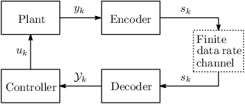
In this section, we state the setup of the control systems and formulate the problem to be solved in this paper.

We consider stabilization of a single-input single-output discrete-time system which has a communication channel at the side of the plant output as depicted in Fig. 1. At time $k$, the encoder observes the plant output $y_{k}\in\mathbb{R}$ and quantizes it. The quantized signal $s_{k}\in\Sigma_{N}$ is transmitted to the decoder through the finite data rate channel. Here, the set $\Sigma_{N}$ represents all possible outputs of the encoder and contains $N$ symbols. Thus, the required data rate is expressed as $R:=\log N$ [bits/sample]. From the received signal $s_{k}$, the decoder computes the interval $\mathcal{Y}_{k}\subset\mathbb{R}$, which is an estimate of $y_{k}$. Finally, using the past and current estimates, the controller provides a control input $u_{k}\in\mathbb{R}$.

In what follows, we describe the details of each component in the system. The plant is an $n$-dimensional autoregressive system whose parameters are uncertain¹¹ 1 The results in this paper can be extended to the case where the plant is a time-varying ARX model as $y_{k+1}=\sum^{n_{y}}_{i=1}a_{i,k}y_{k-i+1}+\sum^{n_{u}}_{i=1}b_{i}u_{k-i+1}$, where $b_{1},\dots,b_{n_{u}}$ are known parameters and $b_{1}\neq 0$. In [15], a related class of plants is studied for limited data rate control.:

Here, for the initial values $y_{k}$, $k=-n+1,-n+2,\dots,0$, there exist known bounds $Y_{k}>0$ as $|y_{k}|\leq Y_{k}$, and the input $u_{k}$ is set to $0$ for $k<0$. Each uncertain parameter $a_{i}$ is represented by the nominal value $a_{i}^{*}$ and the width $\epsilon_{i}\geq 0$ of the perturbation as

Let $A^{*}$ represent the set of parameters $a_{i}$ where each parameter is the nominal one, and let $\lambda_{A^{*}}\!$ be the product of the poles of the plant with the parameters $A^{*}$.

The encoder quantizes the plant output $y_{k}$ into the $N$-alphabet signal $s_{k}\in\Sigma_{N}$, where $\Sigma_{N}:=\{1,2,\dots,N\}$. The input range of the encoder is centered at the origin and the width is defined by a scaling parameter $\sigma_{k}>0$. In particular, the output $s_{k}$ of the encoder is given as

where $q_{N}(\cdot)$ is a static $N$-level quantizer whose input range is $[-1/2,1/2]$. In the quantizer $q_{N}$, it is assumed that boundaries of the quantization cells are symmetric about the origin. This assumption is introduced to avoid complexity in the analysis regarding how large the state estimation sets generated by quantized information become. By its symmetry, the quantizer $q_{N}$ is characterized by the set of boundary points $h_{l}\geq 0$, $l\in\left\{0,1,\dots,\lceil N/2\rceil\right\}$, of nonnegative quantization cells. Here, $\lceil\cdot\rceil$ is the ceiling function. These points must satisfy

The origin $h_{0}$ is a boundary only when the number $N$ of quantization cells is even. However, for simplicity, we use the same notation above even if $N$ is odd. Denote the quantization cells determined by $\{h_{l}\}_{l}$, from left to right, by $\mathcal{C}_{i}$, $i=1,2,\cdots,N$:

(i) If $N$ is odd, then

(ii) If $N$ is even, then

Then, for a given set of boundaries $\{h_{l}\}_{l}$ of the quantizer $q_{N}$ and consequently the quantization cells (5) or (6), we define the outputs of the quantizer as follows:

The decoder converts the received signal $s_{k}$ to the interval $\mathcal{Y}_{k}\subset\mathbb{R}$, which provides an estimate of the set in which the plant output $y_{k}$ should be contained. Formally, $\mathcal{Y}_{k}$ is defined as the interval corresponding to the quantization cell that $y_{k}$ fell in, i.e.,

The controller provides the control input $u_{k}$ based on the estimates $\mathcal{Y}_{k-n+1},\dots,\mathcal{Y}_{k}$ as

where $f_{i,k}(\cdot)$ is an arbitrary map from an interval on $\mathbb{R}$ to a real number.

We remark that the scaling parameter $\sigma_{k}$ should be large enough to cover all possible inputs to the encoder. Otherwise, the quantizer may be saturated, in which case we lose track of the plant output $y_{k}$. On the other hand, if we take $\sigma_{k}$ large, the quantization error also becomes large. Moreover, to achieve stabilization of the system, $\sigma_{k}$ should decay to zero gradually.

We determine the scaling parameter $\sigma_{k}$ as follows. At time $k$, the encoder and the decoder predict the next plant output $y_{k+1}$ based on the observed $\mathcal{Y}_{0},\dots,\mathcal{Y}_{k}$. Let $\mathcal{Y}_{k+1}^{-}\subset\mathbb{R}$ be the set of all possible outputs $y_{k+1}$ of the uncertain system (1). Then the scaling parameter $\sigma_{k+1}$ is chosen such that

where $\mu(\cdot)$ denotes the Lebesgue measure on $\mathbb{R}$.

The prediction set of the plant output $y_{k+1}$ constructed at time $k$ is defined as follows:

Under this definition, our prediction strategy is to use the information regarding $y_{k},\dots,y_{k-n+1}$ independently such that $y_{k-i+1}\in\mathcal{Y}_{k-i+1}$ for each $i=1,2,\dots,n$, where $\mathcal{Y}_{k-i+1}$ is the interval received by the decoder at $k-i+1$. Then, clearly, $\mu(\mathcal{Y}_{k+1}^{-})$ is large enough to include $y_{k+1}$, and is computable on both sides of the channel.

The control objective is to robustly stabilize the networked control system depicted in Fig. 1 for all possible parameters within the bounds in (2).

The problem setup is particularly affected by the consideration of uncertain plants. To overcome the difficulties due to the uncertainty, we have introduced some structures in the plant as well as the controller. In the plant (1), the product of the poles is represented as a single parameter $a_{n}$. As we mentioned in Section 1, the product of the poles plays an important role to describe the bounds on the data rate. Since our objective is to characterize the bounds by the product of the poles, the simple expression of the key parameter helps to reduce the complexity in the analysis.

Similarly, the classes of controllers (9) and prediction sets (11) are employed to pursue an analytical approach and, in particular, to obtain necessary limitations in an explicit formula. Here, we use the information regarding $y_{k-n+1},\dots,y_{k}$ independently. This may make the state estimation somewhat conservative. On the other hand, in related works, e.g., [25, 16, 30], the controller can be an arbitrary causal function. If we use a more general controller or a prediction method that allows us to look at the correlations among them, then the estimation sets $\mathcal{Y}_{k-n+1},\dots,\mathcal{Y}_{k-1}$ from times before the current time $k$ may be updated so that they shrink in size. As a result, the system can be stabilized under a smaller data rate compared with the case employing (9) and (11). We note that it may be possible to minimize the state estimation sets numerically [22]; however, in the case of uncertain plants, it is difficult to do this analytically.

Here, regarding the set $\mathcal{Y}_{k+1}^{-}$, we introduce a useful lemma, which will be referred to in the following sections.

By applying the Brunn-Minkowski inequality [3] to (11), we have $\mu(\mathcal{Y}^{-}_{k+1})\geq\sum_{i=1}^{n}\mu\left(\mathcal{A}_{i}\mathcal{Y}_{k-i+1}\right)$. Furthermore, the equality holds since $\mathcal{A}_{i}\mathcal{Y}_{k-i+1}$, $i=1,\dots,n$, are connected intervals in $\mathbb{R}$ by the definitions in (2) and (8).

∎

In this section, we consider the quantizer (7) using a fixed number $N$ of quantization cells. Under the setup, we present a lower bound on the data rate $R$ as a necessary condition for the system to be stable. The bound is expressed by the level of instability and uncertainty in the plant. It is important to note that the previous works [21, 12, 6] dealing with uncertainties have studied only sufficient conditions which contain some conservativeness.

Before providing the result, we introduce an assumption regarding the poles of the plant.

To describe the main result in this section, we introduce the following notation:

We are now ready to present the necessity result for the static data rate case.

One can confirm that the lower bound $R_{\textnormal{nec}}$ on data rate is monotonically increasing with respect to $|\lambda_{A^{*}}\!|$ and $\epsilon_{n}$. Thus, more unstable dynamics or more uncertainty in the plant will result in higher requirement in communication with a larger data rate. We remark that there is no gap between the two expressions in (15) since $R_{\textnormal{nec}}$ is right continuous with respect to $\epsilon_{n}$ at $\epsilon_{n}=0$.

For the special case where no plant uncertainty, i.e., $\epsilon_{i}=0$ for $i=1,\dots,n$, the bound $R_{\textnormal{nec}}$ takes the well-known form $\log|\lambda_{A^{*}}\!|$. In addition, if all poles lie outside of the unit circle, this bound coincides with those given in [25, 16]. It is interesting to note that for an uncertain plant with $\epsilon_{n}>0$ and $R_{\textnormal{nec}}>1$, the following inequality holds:

That is, even if we assume the most conservative plant dynamics within (2), the bound for the known plants case is looser than the necessary data rate bound $R_{\textnormal{nec}}$.

Moreover, we remark that for the uncertain plants such that $R_{\textnormal{nec}}<1$, we have that $R_{\textnormal{nec}}<\max_{\lambda_{A}\in[\lambda_{A^{*}}\!-\epsilon_{n},\lambda_{A^{*}}\!+\epsilon_{n}]}\log|\lambda_{A}|$. However, we can not construct a quantizer achieving $R<1$ since this implies that the number of the quantization cells $N$ is less than $2$. Thus, the case of $R_{\textnormal{nec}}<1$ may be less interesting from a practical viewpoint.

In the following example, we compare the necessary limitation $R_{\textnormal{nec}}$ with the result for known plants to confirm the gap between the two bounds.

The work [20] shows another special case of Theorem 1. for the case when the quantizer is uniform; the uniform quantizer is the simplest quantizer, which divides the input range into quantization cells of same lengths. If the plant is uncertain with $\epsilon_{n}>0$, then the necessary data rate bound in [20] is higher than that in (15). Therefore, we may stabilize the system with a lower data rate by using a quantizer that is not uniform but more general.

The proof of the Theorem 1 will be presented in the following two sections. Throughout the proof, the central question is as follows: Under the situation where the estimation set of the plant state becomes large due to instability, at least how precise is the quantization required to be to make the estimation set gradually small? To answer this question, in Section 4, we evaluate the expansion rate of the estimation set for a given quantizer. We focus on the effect of $a_{n}$ on the expansion of the estimation set, since $a_{n}$ is equal to the product of the poles of the plant. Then, in Section 5, the optimal quantizer which minimizes the expansion rate is presented.

In this section, we analyze the expansion rate of the state estimation set for a given quantizer whose boundary points are $\{h_{l}\}_{l}$. We first introduce the sequence $w_{l}$, $l=0,1,\dots,\lceil N/2\rceil-1$, as

Then, the next lemma holds as a necessary condition for the quantizer $\{h_{l}\}_{l}$.

First, we show that stability of the system requires convergence of $\sigma_{k}$. For the estimation set $\mathcal{Y}_{k}$, it is obvious that $\max_{y_{k}^{\prime}\in\mathcal{Y}_{k}}|y_{k}^{\prime}|\geq\mu(\mathcal{Y}_{k})/2$. Letting $\delta$ be the smallest width of the quantization cells, we have that $\mu(\mathcal{Y}_{k})\geq\delta\sigma_{k}$. Hence, if $\lim_{k\to\infty}|y_{k}|=0$, then $\lim_{k\to\infty}\sigma_{k}=0$ holds.

In the rest of the proof, we show that (18) is a necessary condition for the convergence of $\sigma_{k}$. Notice that from (10) $\sigma_{k+1}$ is bounded from below by $\mu(\mathcal{Y}_{k+1}^{-})$. Substitution of (12) from Lemma 1 into (10) yields

We next evaluate the far right-hand side of the above inequality. The set $\mathcal{A}_{n}\mathcal{Y}_{k-n+1}$ depends on the boundaries of $\mathcal{A}_{n}$ and $\mathcal{Y}_{k-n+1}$. By (2), we have $\mathcal{A}_{n}=[a_{n}^{*}-\epsilon_{n},a_{n}^{*}+\epsilon_{n}]$. The boundaries of $\mathcal{Y}_{k-n+1}$ vary depending the cell which the output $y_{k-n+1}$ fell in. Let define the index $l_{k-n+1}$ of the cell as follows: For given $\mathcal{Y}_{k}$ and $\sigma_{k}$, let $l_{k}$ be the index of $\mathcal{Y}_{k}$ such that $\inf_{y^{\prime}_{k}\in\mathcal{Y}_{k}}\left|y^{\prime}_{k}/\sigma_{k}\right|=h_{l_{k}}$. We claim that the width $\mu(\mathcal{A}_{n}\mathcal{Y}_{k-n+1})$ can be written as

Here, for simplicity, we assume that $a_{n}^{*}>0$. Notice that from (13), $\mathcal{A}_{n}$ does not contain the origin. By replacing $a_{n}^{*}$ with $|a_{n}^{*}|$ in the discussion, we can obtain the relations for the case $a_{n}^{*}<0$.

To derive (20), we consider the following two cases (i) and (ii) and use basic results of interval arithmetics [14]. Denote the infimum and the supremum of $\mathcal{Y}_{k-n+1}$ by $\underaccent{{\cc@style\underline{\mskip 10.0mu}}}{\mathcal{Y}}_{k-n+1}$ and $\accentset{{\cc@style\underline{\mskip 10.0mu}}}{\mathcal{Y}}_{k-n+1}$, respectively.

(i) $\underaccent{{\cc@style\underline{\mskip 10.0mu}}}{\mathcal{Y}}_{k-n+1}<0<\accentset{{\cc@style\underline{\mskip 10.0mu}}}{\mathcal{Y}}_{k-n+1}$: In this case, from (5), (6), and (8), $N$ is odd and $l_{k-n+1}=0$, or equivalently, $\mathcal{Y}_{k-n+1}=[-h_{1}\sigma_{k-n+1},h_{1}\sigma_{k-n+1})$. Thus, the width of the product of the intervals is computed as follows:

Hence, (20) holds for this case.

(ii) $\underaccent{{\cc@style\underline{\mskip 10.0mu}}}{\mathcal{Y}}_{k-n+1}\geq 0$ or $\accentset{{\cc@style\underline{\mskip 10.0mu}}}{\mathcal{Y}}_{k-n+1}\leq 0$: In this case, $N$ is even or $l_{k-n+1}\neq 0$. First, suppose that $0\leq\underaccent{{\cc@style\underline{\mskip 10.0mu}}}{\mathcal{Y}}_{k-n+1}$. Noticing (13), we have

The same equalities can be established for the case of $\accentset{{\cc@style\underline{\mskip 10.0mu}}}{\mathcal{Y}}_{k-n+1}\leq 0$ by flipping the signs of $\accentset{{\cc@style\underline{\mskip 10.0mu}}}{\mathcal{Y}}_{k-n+1}$ and $\underaccent{{\cc@style\underline{\mskip 10.0mu}}}{\mathcal{Y}}_{k-n+1}$. Thus, we have (20) for this case also.

Finally, by (19) and (20), it holds that $\sigma_{k+1}\geq w_{l_{k-n+1}}\sigma_{k-n+1}$. Since $\sigma_{k}\to 0$ for all possible parameters in (2) and initial values, the maximum of $w_{l_{k-n+1}}$ must be less than $1$, i.e., (18) is necessary. ∎

In the previous section, we have seen a condition for stability on the expansion rate $w_{l}$, which is defined depending on the quantizer. In this section, we find the quantizer that minimizes $\max_{l}w_{l}$ for a fixed $N$. To state such an optimal quantizer, we introduce the quantizer $q^{*}_{N}$ represented by the boundary points $\{h_{l}^{*}\}_{l}$ as follows:

(i) If $\epsilon_{n}>0$, then

where $t:=|\lambda_{A^{*}}\!|/(|\lambda_{A^{*}}\!|-\epsilon_{n})$.

(ii) If $\epsilon_{n}=0$, then

The following lemma holds.

Fig. 3 illustrates the quantization boundaries $\{h^{*}_{l}\}_{l}$ of the optimal $q^{*}_{N}$ when $|\lambda_{A^{*}}\!|=3.0$, $\epsilon_{n}=0.5$, and $N=8$.

We observe that the quantizer takes its quantization cells smaller towards the boundaries $\pm 1/2$ of the input range. This nonuniformity is an outcome of the minimization of $\max_{l}w_{l}$. Intuitively, this characteristic can be explained as follows. For simplicity, consider the case of a scalar plant where the parameter is given as $a\in\mathcal{A}=[a^{*}-\epsilon,a^{*}+\epsilon]$, $a^{*}>0$. Under the control scheme, the plant output $y_{k}$ is quantized and only the cell, or the interval $\mathcal{Y}_{k}$, to which it belongs is known to the controller. After one time step, because of the plant instability, the interval in which the output should be included will expand in width. When the plant model is known, the expansion ratio is constant and is equal to $|a^{*}|$ for any cell. However, with plant uncertainties, the ratio depends on the location of the cell. In particular, cells further away from the origin expands more. This fact is illustrated in Fig. 4(a) when the quantization is uniform. In contrast, when the proposed quantizer $q^{*}_{N}$ is used, the intervals after one step have the same width (see Fig. 4(b)).

Furthermore, the quantizer $q^{*}_{N}$ becomes more nonuniform in the presence of more uncertainties in the plant, expressed with a larger $\epsilon$. This can be seen in the definition of the boundary points $\{h_{l}^{*}\}_{l}$, where the ratio $r$ given in (14) determines the widths of the cells. Note that when $\epsilon=0$, $q^{*}_{N}$ becomes a uniform one as we have seen in (22).

For the general order plants case, the parameter $a$ in the above explanation should be replaced with the $n$th parameter $a_{n}$, which is equal to the product of the poles of the plant and takes the nominal value as $|\lambda_{A^{*}}\!|$. Thus, the proposed quantizer $q^{*}_{N}$ minimizes the maximum width of the intervals expanded by $a_{n}$ and other parameters do not affect the structure of $q^{*}_{N}$. This is because we have focused on the effect of $a_{n}$ in the stability analysis in the proof of Lemma 2. As a consequence, $q^{*}_{N}$ is expressed in a simple form by $|\lambda_{A^{*}}\!|$ and its uncertainty $\epsilon_{n}$.

Finally, it is interesting to note that as we see in Fig. 3, the quantizer $q^{*}_{N}$ has a property in contrast with the logarithmic quantizer studied in [4, 5, 7, 28]; in such quantizers, the quantization cells become small for inputs around the origin and grow exponentially as the input size increases. We also note that other nonuniform quantizers have been studied in [9] and [27], where stabilization of a continuous-time system and a system identification problem over digital communication channels have been respectively investigated.

After some calculation, we have that $w_{l}$ is constant with respect to $l$, i.e.,

if and only if the quantizer is $q^{*}_{N}$. Therefore, it is enough to show that a quantizer which does not satisfy (23) yields a larger $\max_{l}w_{l}$ compared with the case $q^{*}_{N}$. We prove this by contradiction.

For a given quantizer with the boundaries $\{h_{l}\}_{l}$, denote the expansion rates $w_{l}$ under the quantizer by $w_{l}(h)$. Assume that there exists a quantizer $\{g_{l}\}_{l}$ such that (23) is not satisfied and it holds that $\max_{l}w_{l}(g)<\max_{l}w_{l}(h^{*})$. Then, for any $l\in\{0,1,\dots,\lceil N/2\rceil-1\}$,

We now look at the relation between $g_{l}$ and $h_{l}^{*}$ for each $l$. From (4), we have $g_{0}=h^{*}_{0}=0$. Substituting these equations into (17), we obtain

For the case $l=0$ in (24), we have $w_{0}(g)<w_{0}(h^{*})$. Thus, from the above equations, we have that

Furthermore, by (17), it follows that

for $l\in\{1,2,\dots,\lceil N/2\rceil-1\}$. Substitution of these equations into (24) gives

By introducing the relation (25) to the above, we recursively obtain $g_{l}<h^{*}_{l}$ for all $l\in\{1,2,\dots,\lceil N/2\rceil\}$. This contradicts $g_{\lceil N/2\rceil}=h^{*}_{\lceil N/2\rceil}=1/2$ given in (4). Therefore, it follows that $\{h_{l}^{*}\}_{l}$ is the optimal quantizer. ∎

Since we found the quantizer which minimizes $\max_{l}w_{l}$, the lower bound on $N$ satisfying (18) is the necessary condition on the data rate $R$ $(=\log N)$. This is to be proved as the last step of the proof of Theorem 1.

In this proof, we derive the bounds (15) and (16) from (18) in Lemma 2 by employing $q^{*}_{N}$ as the quantizer. First, suppose that $\epsilon_{n}>0$. We consider the following two cases.

(i) $N$ is even: In this case, by the definition of $\{h_{l}^{*}\}_{l}$, we have that $h_{l}^{*}=(1-r^{l})/(1-r^{\lceil N/2\rceil})$. Thus, it holds that $\max_{l}w_{l}={\epsilon_{n}}/(1-r^{\lceil N/2\rceil})$. Consequently, the necessary condition (18) is equivalent to

(ii) $N$ is odd: Similarly, we have that the inequalities

are necessary.

Comparing $N_{\textnormal{nec}}^{(\textnormal{e})}$ with $N_{\textnormal{nec}}^{(\textnormal{o})}$, it is clear that $N_{\textnormal{nec}}^{(\textnormal{o})}>N_{\textnormal{nec}}^{(\textnormal{e})}$. Hence, $N>N_{\textnormal{nec}}^{(\textnormal{e})}$ is necessary for both cases (i) and (ii). From the relation $R=\log N$, we obtain the condition (15).

For the case $\epsilon_{n}=0$, noticing that $\max_{l}w_{l}={|a_{n}^{*}|}/{N}$, we have (15) for this case also. ∎

In this section, we present a sufficient condition for the existence of a stabilizing feedback control scheme under the static data rate. The condition offers a stability test by calculating the spectral radius of a certain matrix.

Given a certain data rate $R$, or $N$, and a static quantizer $\{h_{l}\}_{l}$, we employ the control law as follows: In the encoder (3), the scaling parameter is determined by

and in the controller (9), the control is given as

Here, we denote the supremum and the infimum of $\mathcal{Y}_{k+1}^{-}$ as $\accentset{{\cc@style\underline{\mskip 10.0mu}}}{\mathcal{Y}}^{-}_{k+1}$ and $\underaccent{{\cc@style\underline{\mskip 10.0mu}}}{\mathcal{Y}}^{-}_{k+1}$, respectively.

Next, we introduce some notations required for the analysis of the resulting system. For $i=1,2,\dots,n$, define $w_{i,l}$, $l=0,1,\dots,\lceil N/2\rceil-1$, as follows: If $N$ is odd, $w_{i,0}:=2(|a_{i}^{*}|+\epsilon_{i})h_{1}$, and for $l\geq 1$,

If $N$ is even, $w_{i,l}$ is defined as in (28) for any $l$. We note that $w_{l}$ defined in (17) corresponds to $w_{n,l}$. As we will see in later, $w_{i,l}$ represents the expansion rate of the quantization cells, $[h_{l},h_{l+1})$ and $[-h_{l+1},-h_{l})$, enlarged by the parameter $a_{i}$. We denote by $\accentset{{\cc@style\underline{\mskip 10.0mu}}}{w}_{i}$ the maximum of $w_{i,l}$ over all $l$. Moreover, define the matrix $H\in\mathbb{R}^{n\times n}$ containing $\accentset{{\cc@style\underline{\mskip 10.0mu}}}{w}_{1},\dots,\accentset{{\cc@style\underline{\mskip 10.0mu}}}{w}_{n}$ as

We are now ready to present the main theorem of this section.

We emphasize that the optimal quantizer $q_{N}^{*}$ proposed in Lemma 3 can reduce the sufficient data rate compared with the uniform one, employed in [12, 21, 20]. To confirm this, we now show an example.

First, we show that if $\sigma_{k}\to 0$ then $y_{k}\to 0$ as $k\to\infty$ under the control law. This is easy to establish because by substituting (27) to (1) and by referring to the definition (11) of $\mathcal{Y}_{k+1}^{-}$, we have that

Next, we prove that (33) implies that $\sigma_{k}\to 0$. By (26) and the equality in (12) from Lemma 1, we have

For the $i$th term $\mu\left(\mathcal{A}_{i}\mathcal{Y}_{k-i+1}\right)$, we claim that

Here, $l$ is the index of the boundary of $\mathcal{Y}_{k-i+1}$ closer to the origin, i.e., $l$ is the index such that $h_{l}\sigma_{k-i+1}=\min\{|\accentset{{\cc@style\underline{\mskip 10.0mu}}}{\mathcal{Y}}_{k-i+1}|,\,|\underaccent{{\cc@style\underline{\mskip 10.0mu}}}{\mathcal{Y}}_{k-i+1}|\}$.

To show (35), we first compute $\mathcal{A}_{i}\mathcal{Y}_{k-i+1}$ using basic results in interval arithmetics [14]. Then we have

Furthermore, we consider the following two cases and show (35) from (36) for each case.

(i) $\underaccent{{\cc@style\underline{\mskip 10.0mu}}}{\mathcal{Y}}_{k-i+1}<0<\accentset{{\cc@style\underline{\mskip 10.0mu}}}{\mathcal{Y}}_{k-i+1}$: From the symmetry of the quantizer, $N$ must be odd and $l=0$, and hence, $\mu(\mathcal{Y}_{k-i+1})=2h_{1}\sigma_{k-i+1}$. By substituting this equality to the first case in (36), (35) is established.

(ii) Otherwise: The absolute values of the boundaries of $\mathcal{Y}_{k-i+1}$ are $h_{l}\sigma_{k-i+1}$ and $h_{l+1}\sigma_{k-i+1}$. Noticing that $0\leq h_{l}<h_{l+1}$, we have (35) from (36) for this case also.

By taking the maximum of the right-hand side of (35) over all possible $y_{k-i+1}$, or all $l$, and by (34), we have an upper bound of $\sigma_{k+1}$ as

Here, consider the following linear system

From (37), the bottom element of $\zeta_{k+1}$ is greater than or equal to $\sigma_{k+1}$ for any time $k$. The inequality (33) implies that $H^{k}$ converges to the zero matrix and hence $\sigma_{k}\to 0$ as $k\to\infty$. ∎

Here, we discuss tightness of the derived limitations. We first present the special cases that Theorems 1 and 2 become necessary and sufficient conditions. We then compare tightness of the limitations with that of the existing works dealing with plant uncertainty.

As we have seen in Example 2, in general, there exists a gap between the necessary bound given by Theorem 1 and the sufficient bound obtained from Theorem 2. This gap is caused since, in both necessity and sufficiency analyses, there exist conservativeness in the evaluation of the width of the prediction set $\mathcal{Y}^{-}_{k+1}$.

Theorem 2 becomes a tight condition for stability in the following case: For the class of plants and quantizers where the indices of the quantization cells which result in the maximum expansion rates, i.e., $\arg\max_{l}w_{i,l}$, are the same for all $i=1,2,\dots,n$, the condition (33) is also necessary for stability. This fact is followed by the proof of Theorem 2 and the discussion below. In the proof, we evaluate the width $\mu(\mathcal{Y}^{-}_{k+1})=\sum_{i=1}^{n}\mu(\mathcal{A}_{i}\mathcal{Y}_{k-i+1})$ over all possible $y_{k-n+1},\dots,y_{n}$. As an upper bound on the width, we consider the sum of the maximum $\accentset{{\cc@style\underline{\mskip 10.0mu}}}{w}_{i}\sigma_{k-i+1}$ of each summand $\mu(\mathcal{A}_{i}\mathcal{Y}_{k-i+1})$. When $\arg\max_{l}w_{i,l}$ are the same for all $i$, this upper bound and hence the condition (33) become tight.

References

- [1] B. R. Barmish, New Tools for Robustness of Linear Systems. Macmillan, 1994.
- [2] S. P. Bhattacharyya, H. Chapellat, and L. H. Keel, Robust Control: The Parametric Approach. Prentice-Hall, 1995.
- [3] T. M. Cover and J. A. Thomas, Elements of Information Theory, 2nd ed. Wiley, 2006.
- [4] N. Elia and S. K. Mitter, “Stabilization of linear systems with limited information,” IEEE Trans. Autom. Control, vol. 46, no. 9, pp. 1384–1400, 2001.
- [5] M. Fu and L. Xie, “The sector bound approach to quantized feedback control,” IEEE Trans. Autom. Control, vol. 50, no. 11, pp. 1698–1711, 2005.
- [6] M. Fu and L. Xie, “Quantized feedback control for linear uncertain systems,” Int. J. Robust Nonlin. Control, vol. 20, no. 8, pp. 843–857, 2010.
- [7] T. Hayakawa, H. Ishii, and K. Tsumura, “Adaptive quantized control for linear uncertain discrete-time systems,” Automatica, vol. 45, no. 3, pp. 692–700, 2009.
- [8] V. L. Kharitonov, “Asymptotic stability of an equilibrium position of a family of linear differential equations,” Differential Equations, vol. 14, pp. 1483–1485, 1979.
- [9] K. Li and J. Baillieul, “Robust quantization for digital finite communication bandwidth (DFCB) control,” IEEE Trans. Autom. Control, vol. 49, no. 9, pp. 1573–1584, 2004.
- [10] D. Liberzon and J. P. Hespanha, “Stabilization of nonlinear systems with limited information feedback,” IEEE Trans. Autom. Control, vol. 50, no. 6, pp. 910–915, 2005.
- [11] D. G. Luenberger, Optimization by Vector Space Methods. Wiley, 1997.
- [12] N. C. Martins, M. A. Dahleh, and N. Elia, “Feedback stabilization of uncertain systems in the presence of a direct link,” IEEE Trans. Autom. Control, vol. 51, no. 3, pp. 438–447, 2006.
- [13] P. Minero, M. Franceschetti, S. Dey, and G. N. Nair, “Data rate theorem for stabilization over time-varying feedback channels,” IEEE Trans. Autom. Control, vol. 54, no. 2, pp. 243–255, 2009.
- [14] R. E. Moore, Interval Analysis. Prentice-Hall, 1966.
- [15] G. N. Nair and R. J. Evans, “Stabilization with data-rate-limited feedback: Tightest attainable bounds,” Syst. Control Lett., vol. 41, no. 1, pp. 49–56, 2000.
- [16] G. N. Nair and R. J. Evans, “Stabilizability of stochastic linear systems with finite feedback data rates,” SIAM J. Control Optim., vol. 43, no. 2, pp. 413–436, 2004.
- [17] G. N. Nair, F. Fagnani, S. Zampieri, and R. J. Evans, “Feedback control under data rate constraints: An overview,” Proc. IEEE, vol. 95, no. 1, pp. 108–137, 2007.
- [18] D. Nešić and D. Liberzon, “A unified framework for design and analysis of networked and quantized control systems,” IEEE Trans. Autom. Control, vol. 54, no. 4, pp. 732–747, 2009.
- [19] K. Okano and H. Ishii, “Data rate limitations for stabilization of uncertain systems,” in Proceedings of the 51st IEEE Conference on Decision and Control, 2012, pp. 3286–3291.
- [20] K. Okano and H. Ishii, “Data rate limitations for stabilization of uncertain systems over lossy channels,” in Proc. of the 2012 American Control Conference, 2012, pp. 1260–1265.
- [21] V. N. Phat, J. Jiang, A. V. Savkin, and I. R. Petersen, “Robust stabilization of linear uncertain discrete-time systems via a limited capacity communication channel,” Syst. Control Lett., vol. 53, no. 5, pp. 347–360, 2004.
- [22] J. Rohn, “Systems of linear interval equations,” Linear Algebra Appl., vol. 126, pp. 39–78, 1989.
- [23] H. Shingin and Y. Ohta, “Disturbance rejection with information constraints: Performance limitations of a scalar system for bounded and Gaussian disturbances,” Automatica, vol. 48, no. 6, pp. 1111–1116, 2012.
- [24] S. Tatikonda and S. Mitter, “Control over noisy channels,” IEEE Trans. Autom. Control, vol. 49, no. 7, pp. 1196–1201, 2004.
- [25] S. Tatikonda and S. Mitter, “Control under communication constraints,” IEEE Trans. Autom. Control, vol. 49, no. 7, pp. 1056–1068, 2004.
- [26] S. Tatikonda, A. Sahai, and S. Mitter, “Stochastic linear control over a communication channel,” IEEE Trans. Autom. Control, vol. 49, no. 9, pp. 1549–1561, 2004.
- [27] K. Tsumura, “Optimal quantization of signals for system identification,” IEEE Trans. Autom. Control, vol. 54, no. 12, pp. 2909–2915, 2009.
- [28] K. Tsumura, H. Ishii, and H. Hoshina, “Tradeoffs between quantization and packet loss in networked control of linear systems,” Automatica, vol. 45, no. 12, pp. 2963–2970, 2009.
- [29] W. S. Wong and R. W. Brockett, “Systems with finite communication bandwidth constraints II: Stabilization with limited information feedback,” IEEE Trans. Autom. Control, vol. 44, no. 5, pp. 1049–1053, 1999.
- [30] K. You and L. Xie, “Minimum data rate for mean square stabilization of discrete LTI systems over lossy channels,” IEEE Trans. Autom. Control, vol. 55, no. 10, pp. 2373–2378, 2010.