Solvable random walk model with memory and its relations with Markovian models of anomalous diffusion

We summarize the exact asymptotic results obtained for the MSD, which is the second moment of $P(n,t)$:

$\bullet$ If $\beta>2$, we have:

This result actually applies to any kernel $F(\tau)$ with finite first moment. Thus, diffusion is normal and the main effect of memory is to decrease the diffusion constant compared to that of the memoryless random walk $(q=0)$. The larger $q$ (frequent memory use) and the larger $\langle\tau\rangle_{\infty}$ (better memory), the slower diffusion is.

$\bullet$ If $1<\beta<2$, Eq.(8) above no longer holds since $\langle\tau\rangle_{\infty}=\infty$, making the diffusion constant vanish. Instead, motion is asymptotically subdiffusive:

$\bullet$ If $\beta<1$, diffusion is even slower, logarithmic in time:

In particular, by setting $\beta=0$ in (10) one recovers the result of the uniform preferential visit model [26], $M_{2}(t)\simeq\frac{1-q}{q}\ln t$.

In each case above, we make a scaling hypothesis for the probability density in the long time limit:

where, by construction, $g(x)$ is a normalized scaling function ($\int_{-\infty}^{\infty}g(x)dx=1$) of unit variance ($\int_{-\infty}^{\infty}x^{2}g(x)dx=1$). Although $g(x)$ may not be always obtained explicitly, its properties can be inferred from the asymptotic behavior of the even moments, defined as:

$p$ being a positive integer ($M_{2p+1}(t)=0$ by symmetry). Assuming that Eq. (11) holds, it is easy to see that in the long time limit the moments are given by

where $a_{p}$ is a constant given by $a_{p}=\int_{-\infty}^{\infty}dx\ x^{2p}g(x)$. Obviously, $a_{0}=a_{1}=1$. The constants $a_{p}$ are calculated in Section IV.B, and we find that:

$\bullet$ For $\beta>2$, the scaling function $g(x)$ is Gaussian, i.e.,

for any positive integer $p$.

$\bullet$ For $\beta<1$ (logarithmic diffusion case), the process is also Gaussian asymptotically, namely, $a_{p}/a_{p-1}=2p-1$ as above, despite of the fact that memory is very long ranged and diffusion strongly anomalous. This result is non-trivial: the mechanism that makes $g(x)$ Gaussian is strongly driven by memory and different from the one that leads to Gaussianity in the Central Limit Theorem (previous case).

$\bullet$ In the intermediate case $1<\beta<2$ (anomalous diffusion as $t^{\beta-1}$), $g(x)$ deviates from the Gaussian form. Its moments satisfy:

where

Note that both (14) and (15)-(16) are universal relations, i.e. the corresponding limiting distributions $P(n,t)$ do not depend on $q$ nor on the details of the memory kernel but only on the fact that $F(\tau)\sim\tau^{-\beta}$ at large $\tau$.

Alternatively, expression (15)-(16) can be written using special functions. In this paper we define

By integrating (16) by parts, we have ${\cal I}_{p}(\beta)=-\frac{1}{\mu}+pB\left[p\mu,1-\mu\right]$, with $0<\mu<1$ and where $B(x,y)$ is the Beta function. Using properties of the $\Gamma$ function [49], Eqs. (15)-(16) can be rewritten as:

In the two limiting cases $\mu\rightarrow 1^{-}$ (or $\beta\rightarrow 2^{-}$) and $\mu\rightarrow 0^{+}$ (or $\beta\rightarrow 1^{+}$), Eq.(18) gives back $a_{p}/a_{p-1}\rightarrow 2p-1$, namely, the two Gaussian cases previously mentioned.

By taking the second moment of Eq.(1), we obtain a recursive relation for the mean square displacement:

This equation may not be exactly solvable for all $t$, but we investigate its asymptotic behavior. To show (8)-(10), we write Eq.(19) in the form:

with $C(t)=\sum_{\tau=0}^{t}(1+\tau)^{-\beta}$ and

We notice that a diverging $M_{2}(t)$ in the infinite time limit implies that the terms with large $t^{\prime}$ dominate in the sum (21). Therefore, one may approximate $M_{2}(t^{\prime})$ in the sum by its leading asymptotic form, even at small $t^{\prime}$.

If $\beta>2$, we make the asymptotic ansatz $M_{2}(t)\simeq Kt$, obtaining:

since the two sums above converge. Substituting (23) in (20) and noting that $M_{2}(t+1)-M_{2}(t)\simeq K$, one obtains an equation for $K$, which is easily solved as $K=(1-q)/[1+q\langle\tau\rangle_{\infty}]$. This is result (8), which is displayed in Figure 3 (top). This panel also shows the MSD obtained by iterating the exact Eq. (19) numerically from the initial condition $M_{2}(0)=0$, as well as the MSD obtained from Monte Carlo simulations (both are identical within numerical errors). Figure 3 (bottom) actually shows that the time derivative of the exact MSD tends to the calculated diffusivity $K$. Note that higher order corrections to the linear behavior become more important at finite $t$ as $\beta\rightarrow 2$, and convergence is slower. At $\beta=2$, $\langle\tau\rangle_{\infty}=\infty$ and the diffusivity $K$ vanishes, suggesting a change of temporal behavior.

To examine the case $1<\beta<2$, we make the general ansatz $M_{2}(t)\simeq Kt^{\nu}$, where $\nu$ and $K$ are unknown. Similarly to (23), we seek to expand the memory term as ${\cal F}\{Kt^{\nu}\}\simeq Kt^{\nu}(c_{1}+c_{2}t^{-\beta+1})$ for large $t$. As shown in the Appendix B:

The normalization constant $C(t)$ can be written as:

Assuming that $\nu<1$ (subdiffusive behavior), so that we can neglect $M_{2}(t+1)-M_{2}(t)\simeq\dot{M}_{2}(t)$ in (20) compared to the constant $-(1-q)$, and substituting (24) and (25) in (20) we obtain:

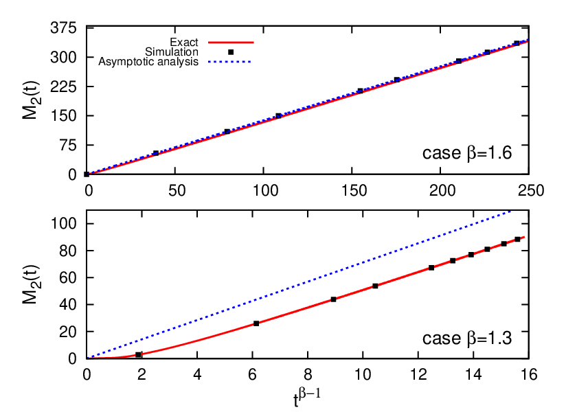
The exponent of $t$ in the right-hand-side of (26) must be 0 for consistency, which gives $\nu=\beta-1\equiv\mu$. Consequently, this equation can be solved for the constant $K$ and formula (9) is obtained. Figure 4 (top) shows that the exact numerical MSD obtained from iterating (19) tends to a linear behavior with respect to the variable $t^{\beta-1}$, as predicted by our result. Note that at large but finite time, the exact MSD would be better approximated by the the leading asymptotic result plus a constant, which unfortunately cannot be calculated by our method (this situation occurs for $\beta<1$ as well, see Fig. 5 below). However, such constant becomes negligible as $t\rightarrow\infty$. For a more precise comparison, we have displayed in Figure 4 (bottom) the derivative of the MSD with respect to $t^{\beta-1}$: this quantity tends to a constant in very good agreement with the calculated $K$.

In the case $\beta<1$, we follow a similar route, now with a logarithmic ansatz $M_{2}(t)\simeq K\ln t$, as suggested by the exact result for the preferential visit model, i.e., $\beta=0$ [26]. Since $\sum_{\tau=0}^{t}(1+\tau)^{-\beta}$ does not converge, one can use directly the Euler-Maclaurin expansion:

at large $t$. Similarly,

where $A$ is some constant. Making the change $t^{\prime}=ut$ and noticing that the functions $\ln u/(1-u)^{\beta}$ and $1/(1-u)^{\beta}$ are integrable both in $0$ and $1$ when $\beta<1$, we obtain, for $t$ large:

By substituting (27) and (29) in (20) and neglecting $M_{2}(t+1)-M_{2}(t)$ as before, we obtain:

which gives the constant $K$ and result (10). Figure 5 (top) shows that the exact MSD obtained numerically becomes a linear function of $\ln t$ at large times, in agreement with theory. We have also displayed in Figure 5 (bottom) the derivative of the MSD with respect to $\ln t$: this quantity tends to a constant in very good agreement with the calculated $K$.

In a similar way, we now consider the asymptotic behavior of the moments $M_{2p}(t)$. We start from the exact relation which follows from the master equation (1):

Assuming the scaling hypothesis (13), and given that $M_{2}(t)$ always diverges as $t\rightarrow\infty$, we can neglect the term $1-q$ as well as the terms proportional to $M_{2k}(t)$ for all $k<p-1$ in the right-hand-side of (31). Substituting $M_{2p}(t+1)-M_{2p}(t)$ by $dM_{2p}/dt$ in the long time limit, Eq. (31) becomes:

If $1<\beta<2$, we have $M_{2}(t)\simeq Kt^{\beta-1}$ and Eq.(32) reads:

Using formula (24), we obtain:

whereas

Since $1<\beta<2$, then $t^{(\beta-1)p-1}\ll t^{(\beta-1)(p-1)}$ and the left-hand-side of Eq.(33) can be neglected. Substituting (34) and (35) in (33), then taking the limit $C(t)\rightarrow\zeta(\beta)$ at large $t$ and using the expression (9) for $K$, Eq. (15) is obtained.

For the case $\beta<1$, or $M_{2}(t)\simeq K\ln t$, the derivative in the left-hand-side of (32) is $O(\ln^{p-1}(t)/t)\rightarrow 0$ and can still be neglected compared with terms growing with time in this equation. Thus Eq.(32) becomes:

where in this case the diverging sums have been replaced by integrals. We next write:

where in the last step we have retained only the first two dominant terms of the binomial expansion, i.e. those of indices $k=0$ and $k=1$. We also have:

Substituting (37) and (38) in (36), then using the expansion $C(t)\simeq t^{1-\beta}/(1-\beta)$ as well as the expression (10) for $K$, one obtains the simple result:

which corresponds to the Gaussian distribution.

Note that the equation that leads to this Gaussian result [Eq. (36)] can be understood as a balance between diffusion due to random increments (the combinatorial left-hand-side) and confining effects due to recurrent memory (the integral right-hand-side). This balance arises because the term $a_{p}dM_{2}(t)^{p}/dt$ in Eq. (32) is negligible. In the simple random walk, on the contrary, $a_{p}dM_{2}(t)^{p}/dt$ is dominant, since $M_{2}(t)\propto t$, and equals the combinatorial term (in the absence of a memory term). Therefore, the mechanism leading to Gaussianity in the memory walk here is very different from the Central Limit Theorem case.

Figure 6 shows several analytical curves $a_{p}/a_{p-1}$ as a function of $\beta$, summarizing the 3 regimes discussed above. To check these results, we performed Monte Carlo simulations of the model and computed the quantity

after obtaining the corresponding moments by averaging $X_{t}^{2p}$, $X_{t}^{2p-2}$ and $X_{t}^{2}$, over many independent walks. If the scaling hypothesis holds, $Q_{p}(t)\rightarrow a_{p}/a_{p-1}$. In each case, we checked that $Q_{p}(t)$ tended to a constant at large times, which is indicated by a dot in Figure 6.

The agreement between theory and simulations is very good. Note, however, that when $\beta$ becomes small ($\beta<1.3$), the computed $Q_{p}(t)$ tends to be larger than the theoretical value. This is because diffusion is very slow in these cases and therefore the scaling regime becomes very difficult to reach in finite time simulations. Recall that the scaling regime settles only when $M_{2}(t)\gg 1$. In ref. [26], the approach toward the scaling regime was studied in details for the case $\beta=0$. It was shown that the first correction to scaling slowly decayed as $1/\ln t$ and thus could be neglected only at extremely long times, which cannot be reached in practice in simulations.

As an additional test, we solved Eq.(1) numerically, calculated the moments from $P(n,t)$, and then calculated $Q_{p}(t)$. The results are indicated by crosses in Fig. 6. The necessary computer memory scales as $t^{2}$ in this method, and times beyond $t=15,000$ could not be reached in practice (this is a low value, compared to $t=10^{6}$ used in simulations). The scaling regime is thus less easy to observe, specially in the subdiffusive case, and the discrepancy with the theoretical $a_{p}/a_{p-1}$ is a bit larger than in simulations.

The subdiffusive law (9) is the consequence of a diverging average backward time $\langle\tau\rangle_{t}$ as $t\rightarrow\infty$. Interestingly, this situation is analogous to that of the continuous time random walk (CTRW), where subdiffusion arises due to diverging waiting times [50, 51]. In this well-known renewal Markovian process, an unbiased random walker remains at its current location during a random time $\tau$, i.i.d. from a distribution $\psi(\tau)$, before performing the next step to a nearest-neighbor site [43]. If $\psi(\tau)\sim\tau^{-\beta}$ with $1<\beta<2$ (or, setting $\beta=1+\mu$, if $0<\mu<1$), then $\langle\tau\rangle=\infty$ and a diffusion constant cannot be properly defined. In this case, motion is subdiffusive with $M_{2}(t)\sim t^{\beta-1}$, the same scaling as in Eq. (9).

The following qualitative argument can be made to explain the similar behaviors of the mean square displacements in these two models. Let us consider a walker in our model starting from the origin $O$ and taking a relocation step at a time $t$ (Figure 7, left). This step, represented by the arrow, brings the walker back to some position $O^{\prime}$ that was occupied earlier, $\tau$ time units before time $t$, where $\tau$ is a random variable $\leq t$ drawn from the p.d.f. $F(\tau)\propto\tau^{-\beta}$. Just before taking this step, the walker was at some distance from the origin, represented by the large circle. In order to reach this circle again from $O^{\prime}$, the walker will typically need to diffuse during another time interval $\tau$ again (assuming stationarity in the process). Hence, only at time about $t+\tau$ the walker’s displacement may grow beyond the radius of the circle. This situation can be seen as analogous to keeping the walker immobile at the position reached at $t$ during a time $\tau$, which is the basic rule of the CTRW (Figure 7, right).

However, one may intuitively guess that the two models differ quantitatively, namely, that their probability densities $P(n,t)$ are given by different scaling functions $g(x)$. This is actually the case, since $g(x)$ is exponential when $\beta\rightarrow 1$ in the one-dimensional CTRW, i.e., $g^{CTRW}(x)\rightarrow\frac{1}{\sqrt{2}}\exp(-\sqrt{2}|x|)$ [11], instead of the Gaussian form in the memory model. More generally, for $1<\beta<2$ the expression of $g^{CTRW}(x)$ is exactly known in terms of the fully asymmetric Lévy law of index $(\beta-1)/2$. Its moments can be calculated exactly, giving [11]:

The above expression is indeed different from (15) or (18). The limit distribution $g(x)$ in the present model does not reduce, to our knowledge, to a standard distribution. Figure 6 displays $a_{p}/a_{p-1}$ as a function of $\beta$ for $p=2,3$ and $4$ for the CTRW and the present model, in which deviations from Gaussianity are weaker.

Further insights on $g(x)$ in the memory model can be gained by studying its behavior at large $x$ for $\beta$ in the range $(1,2)$. This asymptotic behavior can be derived by analyzing the moments in the limit $p\gg 1$. Knowing the properties of $g(x)$ is also useful to understand how the distribution tends to a Gaussian instead of a exponential as $\beta\rightarrow 1^{+}$.

The large $p$ behavior of (18) for any $0<\mu<1$ can be obtained by using the Stirling formula $\Gamma(az+b)\simeq\sqrt{2\pi}e^{-az}(az)^{az+b-1/2}$ for large $z$:

Clearly, the asymptotic result (42) is valid as long as $\chi_{\mu}$ is non-zero. This prefactor is strictly positive if $0<\mu\leq 1$ but vanishes at $\mu=0$ and this case will deserve a special attention below.

If $0<\mu<1$, equation (42) implies that the scaling function follows at large $x$ the leading behavior:

with

Let us notice that the large $x$ behavior above is similar to that of the CTRW with a waiting time distribution $\psi(\tau)\sim\tau^{-(1+\mu)}$. Namely, the leading part of $g^{CTRW}(x)$ is also of the form (43) and with the same exponent $\delta_{\mu}$ as given by (44). This property stems from the fact that the moment relation for CTRW, Eq.(41), also becomes proportional to $p^{2-\mu}$ at large $p$, like in (42). However, the scaling functions do differ in the two models since the prefactors $\chi_{\mu}$ (and therefore $b_{\mu}$ in the exponential) are different.

This difference increases drastically as $\mu\rightarrow 0$: it is easy to see from (42) that

whereas $\chi_{\mu=0}^{CTRW}$ is $>0$. The fact that the prefactor vanishes is a crucial property of the memory model. It indicates that the leading term of the scaling function at large $x$ is no longer given by (43)-(44). A higher order calculation shows that, for any $p$:

which confirms our previous result that $g(x)$ becomes Gaussian again at $\mu=0$. An expansion of the moment relation (18) at large $p$ and small $\mu$ generalizes Eq.(42):

Therefore the exponential behavior of $g(x)$ at large $x$ (i.e. $a_{p}/a_{p-1}\propto p^{2}$ for large $p$) is avoided at $\mu=0$ due to the vanishing prefactor and the distribution adopts a Gaussian profile instead.

References

- [1] E. Bolthausen and U. Schmock, Ann. Probab. 25, 531 (1997).
- [2] H. G. Othmer and A. Stevens, SIAM J. Appl. Math. 57, 1044 (1997).
- [3] R. Pemantle, Probab. Surv. 4 1, (2007).
- [4] A. O. Gautestad and I. Mysterud, Am. Nat. 165, 44 (2005).
- [5] A. O. Gautestad and I. Mysterud, Ecol. Complex. 3, 44 (2006).
- [6] B. Davis, Probab. Theor. Related Fields 84, 203 (1990).
- [7] A. Ordemann, E. Tomer, G. Berkolaiko, S. Havlin, and A. Bunde, Phys. Rev. E 64, 046117 (2001).
- [8] J. W. Lee, J. Phys A: Math. Gen. 31, 3929 (1998).
- [9] J. G. Foster, P. Grassberger, and M. Paczuski, New J. Phys. 11, 023009 (2009).
- [10] J. Choi, J. I. Sohn, K. I. Goh, I. M. Kim, EPL 99, 50001 (2012).
- [11] J.-P. Bouchaud and A. Georges, Phys. Rep. 195, 127 (1990).
- [12] R. Metzler and J. Klafter, Phys. Rep. 339, 1 (2000).
- [13] G. M. Schtz and S. Trimper, Phys. Rev. E 70, 045101 (R) (2004).
- [14] J. C. Cressoni, M. A. A. da Silva, and G. M. Viswanathan, Phys. Rev. Lett. 98, 070603 (2007).
- [15] M. Serva, Phys. Rev. E 88, 052141 (2013).
- [16] L. Peliti, J. Phys 46, 1469 (1985).
- [17] L. Peliti and L. Pietronero, Riv. Nuovo Cimento 10, 1 (1987).
- [18] V. B. Sapozhdcov, J. Phys. A: Math. Gen. 27, L151 (1994).
- [19] C. Song, T. Koren, P. Wang and A.-L. Barabási, Nature Phys. 6, 818 (2010).
- [20] R. Nathan et al., Proc. Natl. Acad. Sci. USA 105, 19052 (2008).
- [21] D. W. Sims et al., Nature 451, 1098 (2008).
- [22] N. E. Humphries, H. Weimerskirch, N. Queiroz, E. J. Southall, and D. W. Sims, Proc. Natl. Acad. Sci. USA 109, 7169 (2012).
- [23] D. Brockmann, L. Hufnagel and T. Geisel, Nature 439, 462 (2006).
- [24] M. C. González, C. A. Hidalgo and A.-L. Barabási, Nature 453, 779 (2008).
- [25] C. Song, Z. Qu, N. Blumm and A.-L. Barabási, Science 327, 1018 (2010).
- [26] D. Boyer and C. Solis-Salas, Phys. Rev. Lett. 112, 240601 (2014).
- [27] J. A. Merkle, D. Fortin, and J. M. Morales, Ecol. Lett. 17, 924 (2014).
- [28] P. R. Moorcroft and M. A. Lewis, Mechanistic home range analysis (Princeton University Press, Princeton, 2006).
- [29] L. Brger, B. D. Dalziel and J. M. Fryxell, Ecol. Lett. 11, 637 (2008).
- [30] B. van Moorter et al., Oikos 118, 641 (2009).
- [31] D. Boyer and P. D. Walsh, Phil. Trans. R. Soc. A 368, 5645 (2010).
- [32] J. Nabe-Nielsen, J. Tougaard, J. Teilmann, K. Lucke, and M. C. Forchhammer, Oikos 122, 1307 (2013).
- [33] P. Turchin, Quantitative analysis of movement. (Sunderland, MA. Sinauer Associates Inc, 1998).
- [34] E. A. Codling, M. J. Plank, and S. Benhamou, J. R. Soc. Interface 5, 813 (2008).
- [35] G. M. Viswanathan, M. G. E. da Luz, E. P. Raposo, and H. E. Stanley, The Physics of foraging (Cambridge, Cambridge, 2011).
- [36] O. Bénichou, M. Coppey, M. Moreau, P.-H. Suet, and R. Voituriez, Phys. Rev. Lett. 94, 198101 (2005).
- [37] O. Bénichou, C. Loverdo, M. Moreau, and R. Voituriez, Rev. Mod. Phys. 83, 81 (2011).
- [38] F. Bartumeus, Oikos 118, 488 (2009).
- [39] J. M. Morales, D. T. Haydon, J. Frair, K. E. Holsinger, J. M. Fryxell, Ecology 85, 2436 (2004).
- [40] G. M. Viswanathan, E. P. Raposo, M. G. E. da Luz, Phys. Life Rev. 5, 133 (2008).
- [41] F. Bartumeus, M. G. E. da Luz, G. M. Viswanathan, J. Catalan, Ecology 86, 3078 (2005).
- [42] I. Rhee, M. Shin, S. Hong, K. Lee, and S. Chong, IEEE/ACM Trans. Netw. 19, 630 (2011).
- [43] E. W. Montroll and G. H. Weiss, J. Math. Phys. 6, 167 (1965).
- [44] S. C. Lim and S. V. Muniandy, Phys. Rev. E 66, 021114 (2002).
- [45] G. U. Yule, Phil. Trans. R. Soc. (London) B 213, 21 (1925)..
- [46] A.-L. Barabási and R. Albert, Science 286, 509 (1999).
- [47] P. L. Krapivsky, S. Redner, and F. Leyvraz, Phys. Rev. Lett. 85, 4629 (2000).
- [48] M. R. Evans and S. N. Majumdar, Phys. Rev. Lett. 106, 160601 (2011).
- [49] Namely, , and .
- [50] M. F. Shlesinger, J. Stat. Phys. 10, 421 (1974).
- [51] M. Kotulski, J. Stat. Phys. 81, 777 (1995).
- [52] Y. He, S. Burov, R. Metzler, and E. Barkai, Phys. Rev. Lett. 101, 058101 (2008).
- [53] A. Rebenshtok and E. Barkai, Phys. Rev. Lett. 99, 210601 (2007).
- [54] A. Lubelski, I. M. Sokolov, and J. Klafter, Phys. Rev. Lett. 100, 250602 (2008).
- [55] F. Thiel and I. M. Sokolov, Phys. Rev. E 89, 012115 (2014).
- [56] J.-H. Jeon, A. V.Checkin, R. Metzler, arXiv:1405.2193 [cond-mat.stat-mech] (2014).
- [57] M. A. A. da Silva, J. C. Cressoni, G. M. Schtz, G. M. Viswanathan, and S. Trimper, Phys. Rev. E 88, 022115 (2013).
- [58] D. Boyer, M. C. Crofoot and P. D. Walsh, J. R. Soc. Interface 9, 842-847 (2012).