Loose Legendrian and Pseudo-Legendrian Knots in 3-Manifolds
Abstract.
We prove a complete classification theorem for loose Legendrian knots in an oriented 3-manifold, generalizing results of Dymara and Ding-Geiges. Our approach is to classify knots in a -manifold that are transverse to a nowhere-zero vector field up to the corresponding isotopy relation. Such knots are called -transverse. A framed isotopy class is simple if any two -transverse knots in that class which are homotopic through -transverse immersions are -transverse isotopic. We show that all knot types in are simple if any one of the following three conditions hold: is closed, irreducible and atoroidal; or the Euler class of the -bundle orthogonal to is a torsion class, or if is a coorienting vector field of a tight contact structure. Finally, we construct examples of pairs of homotopic knot types such that one is simple and one is not. As a consequence of the -principle for Legendrian immersions, we also construct knot types which are not Legendrian simple.
1. Introduction
We work in the smooth category. Throughout this paper is an oriented, connected -manifold, which is not necessarily compact. We fix an auxillary Riemannian metric on .
Let be a cooriented contact structure on . For Legendrain knots in with well-defined rotation and Thurston-Bennequin numbers, one classical problem is: Given an ordered pair , and a smooth knot type , classify the Legendrian knots such that and . This is sometimes referred to as the botany problem [15]. The Thurston-Bennequin number of a Legendrian knot is defined when is zero-homologous in . The rotation number is defined either when is zero-homologous in , or when is a trivializable 2-plane bundle.
We study the following generalized botany problem, which applies to all knot types in any contact manifold with a cooriented contact structure : Given a connected component of the space of framed knots, and a connected component of the space of Legendrian immersed curves , classify the Legendrian knot types in . (The framing of a Legendrian knot is given by orthogonally projecting a coorienting vector field for the contact structure to the normal bundle of .) This generalizes the botany problem because two smoothly isotopic Legendrain knots and with well-defined Thurston-Bennequin numbers are isotopic as framed knots if and only if , and similarly, two Legendrian knots with well-defined rotation numbers which are homotopic as immersed curves are homotopic as Legendrian immersed curves if and only if . We study this generalized botany problem by classifying knots transverse to a nowhere-zero vector field on ; we call these -transverse knots.
Throughout the article, we use the following notation and terminology. All spaces of knots and curves are equipped with the -topology. Connected components of a space of knots or immersed curves are referred to as isotopy or homotopy classes, respectively. A smooth isotopy class is denoted . An isotopy class of framed, Legendrian, or -transverse knots is denoted , , or , respectively. A homotopy class of framed, Legendrian, or -transverse immersed curves is denoted , , or , respectively.
A Legendrian knot in an overtwisted contact manifold is loose if it is contained in the complement of some overtwisted disk . Otherwise, is non-loose.
We give a complete solution to the generalized botany problem for loose Legendrian knots.
Prior results of Dymara and Ding-Geiges suggest that, in the case of loose knots, classical invariants, and their generalizations discussed above, completely determine the Legendrian knot type. Dymara [10, 11] proved that if the 2-plane bundle is trivializable, and the smooth knot type has infinitely many framings, then two loose Legendrian knots and in are isotopic as framed knots and homotopic through Legendrian immersions if and only if they are Legendrian isotopic. The number of framings of a smooth knot type is the number of distinct isotopy classes of framed knots with underlying smooth knot type . Ding and Geiges [8] generalized Dymara’s theorem. They proved that if has infinitely many framings, and the connected component of the space of framed curves containing and contains infinitely many distinct connected components of the space of Legendrian immersions (this is true, e.g., when is trivializable), then and are isotopic as framed knots and homotopic through Legendrian immersions if and only if they are Legendrian isotopic.
We first prove a best-possible generalization of the results of Dymara and Ding-Geiges. Our generalization does not make any assumption on the number of framings of or about the number of components of the space of Legendrian immersions in . Our proof uses an -principle of Cieliebak and Eliashberg [7].
1 Theorem (cf. Theorems 11.2 and 11.3 in the text).
Let be a 3-manifold with a cooriented contact structure , and let be an overtwisted disk in . Let and be two smoothly isotopic Legendrian knots in . Assume that the following three conditions hold:
- (1)
and are isotopic as framed knots,
- (2)
and are homotopic as Legendrian immersions,
- (3)
where is a coorienting vector field of .
Then and are isotopic as Legendrian knots.
In item (3), and are homomorphisms from the fundamental groups of the spaces of framed knots and immersed curves in , respectively, to ; these homomorphisms are defined in Section 4, and we compute them explicitly in many examples.
Conversely, we construct examples of Legendrian knots which are not Legendrian isotopic, but are isotopic as framed knots and homotopic through Legendrian immersions. These examples arise when , and the knots in these examples can be chosen to be loose.
Our approach is to study a version of the botany problem for a more general class of knots, which we call –transverse knots. We say that a knot or immersed curve is -transverse if the velocity vector and the vector span a -plane for all . In the special case where is a coorienting vector field for a contact structure on , is called pseudo-Legendrian; this notion was introduced by Benedetti and Petronio [2, 3].
We begin by proving Theorem 2, a general classification theorem for -transverse knots in oriented -manifolds, which is the primary tool used in the proof of Theorem 1. To state Theorem 2, we introduce a local operation on -transverse immersed curves. Let be a -transverse immersed curve in . Consider a coordinate chart such that contains an unknotted arc of and Let denote the -transverse knot obtained from by adding of the kink-pairs shown on the top in Figure 1 along this arc of , if , and of the kink-pairs on the bottom, if . In Lemma 3.6, we prove that is a transitive -action on the set of -transverse homotopy classes in a given connected component of the space of framed curves in , and also on the set of -transverse isotopy classes in a given connected component of the space of framed knots in .
This kinking operation is related to, but not the same as, the usual stabilization operation on Legendrian knots. The usual stabilization operation occurs in a chart on which is contactomorphic to where ; such a chart exists at every point of by the Darboux Theorem. Given a Legendrian knot in and positive integer , let (respectively, ) be the Legendrian knot obtained by performing positive (respectively, negative) stabilizations on , as shown in Figure 2. Working in the Lagrangian projection, and using the isotopy in Figure 5, it is straightforward to check that and are isotopic as -transverse knots, where again Since is a coorienting vector field for , this -transverse isotopy is a pseudo-Legendrian isotopy.
The above -action appears in Theorem 2, a classification theorem for -transverse knots in a 3-manifold. This theorem answers the -transverse version of the botany problem: Classify the -transverse knot types in a given framed isotopy class and a given connected component of the space of -transverse immersed curves. (The framing of a -transverse knot is given by orthogonally projecting to the normal bundle of ).
2 Theorem (cf. Theorem 4.6 in the text).
Let be an oriented -manifold and let be a non-vanishing vector field on . Let be a -transverse knot in , contained in the framed isotopy class , the framed homotopy class , and the -transverse homotopy class . Let and be the homotopy and isotopy kink-cancelling homomorphisms discussed in detail in Section 4.
- •
The set of -transverse homotopy classes in is a -torsor.
- •
The set of -transverse isotopy classes in is a -torsor.
- •
The set of -transverse isotopy classes in is a -torsor.
The maps and are defined as half the values of the Euler class of on the class of realized by fundamental class of pushed forward by the adjoint map of the loops in and respectively.
The intuition behind Theorem 2 is as follows. For a fixed -transverse knot , the knots defined by the kinking operation are always isotopic as framed knots. Suppose is a -transverse knot in with . In this case, the knots are all distinct as -transverse immersed curves (and hence also as -transverse knots), due to the fact that their projections to the -plane have different rotation numbers. However, in an arbitrary oriented 3-manifold with nowhere-zero vector field , it may happen that and are homotopic as -transverse curves. We prove this happens precisely when there is a framed self-homotopy of along which the Euler class of the 2-plane bundle takes the value (in this case ). Moreover, it may happen that and are distinct as -transverse knots; we prove this happens precisely when there is no framed self-isotopy of on which the Euler class of the 2-plane bundle takes the value (in this case is not in the image of ). In particular, we get the following Corollary to Theorem 2.
3 Corollary (cf. Corollary 4.7 in the text).
The number of -transverse knot types in a given framed isotopy class which are homotopic through -transverse immersions is the index of in .
In this index is 1. In the examples in this paper, the index is either or infinite. We do not know whether other values are possible.
We call a framed isotopy class simple if any two -transverse knots and in which are homotopic through -transverse immersions are isotopic as -transverse knots. Theorem 2 allows us to determine exactly when a framed knot type is simple; see Corollary 4.
4 Corollary (cf. Corollary 4.8 in the text).
The framed isotopy class is simple if and only if . In particular, this is the case when .
Next we describe three types of examples. First, we describe manifolds and vector fields such that every framed knot type in is simple.
5 Theorem (cf. Theorem 6.1 in the text).
Let be a nowhere-zero vector field on an oriented -manifold satisfying one of the following three conditions:
- (1)
The Euler class is a torsion element, or in particular, if .
- (2)
The manifold is closed, irreducible and atoroidal.
- (3)
is a coorienting vector field of a contact structure such that is tight, or more generally, such that is a covering of a tight contact manifold.
Then every framed isotopy class in is simple.
Second, we give examples of nonsimple classes. In our first set of examples, for an infinite family of vector fields with distinct Euler classes, we describe a framed homotopy class of immersed curves such that every framed knot type in this class is nonsimple.
6 Theorem (cf. Theorem 9.5 in the text).
Let be an -bundle over a non-orientable surface of genus with oriented total space, and be the solid curve pictured in Figure 9. Let be any homotopy class (connected component of the space) of framed immersions in that contains a curve projecting to Then for any nonzero there exists a nowhere-zero vector field on such that no framed knot type in is simple. In particular, for any -transverse knot in , the -transverse knots and are homotopic through -transverse immersions, isotopic as framed knots, and not isotopic through -transverse knots.
As a corollary to Theorem 6, we construct knot types which are not Legendrian simple. Eliashberg [12] proved that every 2-plane field is homotopic to an overtwisted contact structure. Hence the vector field above can be chosen to be a coorienting vector field of an overtwisted contact structure on .
7 Corollary (cf. Corollary 9.6 in the text).
Let be an oriented 3-manifold as in Theorem 9.5 with a cooriented contact structure homotopic to the 2-plane field . For each framed knot type containing a Legendrian representative , the stabilized Legendrian knots and are isotopic as framed knots, and homotopic as Legendrian immersions, but not isotopic as Legendrian knots; these Legendrian knots can be chosen to be loose.
Third, we describe a framed homotopy class of immersed curves which contains both simple and nonsimple framed knot types, again for an infinite family of vector fields with distinct Euler classes. The proof of this theorem uses an invariant of properly immersed annuli in -manifolds with boundary defined by Schneiderman [20].
8 Theorem (cf. Theorem 10.5 in the text).
Let be an -bundle over an orientable surface of genus . Let be the framed isotopy class of the fiber with any framing, and let be the framed isotopy class obtained from by a finger move around a curve projecting to the loop on ; see Figures 10 and 11. Then for any nonzero there exists a nowhere-zero vector field such that the framed knot type of is simple in while the knot type is not. In particular, there are -transverse knots and in which are homotopic through -transverse immersions, isotopic as framed knots, and not isotopic through -transverse knots.
Again, by choosing a contact structure on with coorienting vector field , we construct examples of knot types which are not Legendrian simple.
9 Corollary (cf. Corollary 10.6 in the text).
Let be an oriented 3-manifold as in Theorem 10.5, with a cooriented contact structure homotopic to the 2-plane field . Let be a Legendrian knot which is smoothly isotopic to the knot in Theorem 10.5. Then the stabilized Legendrian knots and are isotopic as framed knots, and homotopic as Legendrian immersions, but not isotopic as Legendrian knots; these Legendrian knots can be chosen to be loose.
The structure of the paper is as follows. In Section 2, we review Trace’s theorem for knots in and explain why our classification theorem generalizes it. In Section 3, we review basic facts of framed and -transverse isotopy, and introduce the actions which appear in the main classification theorem. In Section 4, we introduce the homomorphisms and and prove the classification theorem. In Section 6, we prove Theorem 6.1. In Section 7, we discuss facts about the fundamental groups of the spaces of framed knots and immersions in , which we use to construct the examples in the next two theorems. Section 8 is a brief expository section which is helpful for visualizing the examples in the next two theorems. Sections 9, 10, and 11 contain proofs of Theorems 6, 8, and 1, respectively. The last section is an appendix on -principles.
2. Classical Invariants of -Transverse Knots
Consider a knot in transverse to the vertical vector field . Consider the following two “classical” invariants of : The rotation number of the projection of to the -plane, and the self-linking number of , where is the knot framed by . Trace [23] proved that such -transverse knots are determined by their classical invariants. We restate his theorem using our terminology.
2.1 Theorem (Trace).
Let . Two -transverse knots and in are isotopic as -transverse knots if and only if
- (1)
and are isotopic as smooth knots,
- (2)
and have the same self-linking number, and
- (3)
the projections of and to the -plane have the same rotation number.
The second and third hypothesis above do not make sense in arbitrary . A rotation number of a -transverse knot can only be defined given a trivialization of the -plane bundle , as the degree of the map which sends a point to the normalized projection of the velocity vector to . The self-linking number is only defined for zero-homologous . When is not zero-homologous, one can instead use the affine self-linking invariant constructed by the second author [5] which generalizes the ordinary self-linking number for zero-homologous knots and makes sense much more generally.
An even more general approach is to replace the first two hypotheses with the hypothesis that and be isotopic as framed knots, and replace the third hypothesis with the hypothesis that and are homotopic through -transverse immersions. These hypotheses make sense in any and are equivalent to Trace’s hypothesis in .
Thus a generalization of Trace’s theorem should characterize when two -transverse knots, which are homotopic through -transverse immersions and isotopic as framed knots with framing given by , are isotopic through -transverse knots.
3. Basic Properties of Framed and -Transverse Isotopy
Let be a -manifold. A framed curve or framed immersion in is an immersion together with a nonvanishing section of the normal bundle to for each . A framed knot is a framed curve which is also an embedding. The space of framed curves in always has two connected components corresponding to each connected component of the space of immersions of into . The space of framed knots may have finitely or infinitely many connected components corresponding to a given connected component of the space of knots in (a given framed isotopy class). Both spaces are equipped with the topology.
3.1 Proposition (Cf. [4]).
Let be any -manifold. There are two components of the space of framed curves corresponding to each component of the space of unframed curves in .
Proof. Consider the Stiefel bundle of orthonormal -frames over . The fiber is . Let be a framed curve in . Lift to a curve in using the frame given by where is the framing vector of at time . Since each fiber of is an there is a canonical line bundle over . The first Stiefel-Whitney class of this bundle is an element of . Its value on the lift of and the lift of with one extra twist of its framing differ by 1. Thus the number of connected components corresponding to each component of the space of unframed curves in is at least two.
Since there is an obvious homotopy between the curve with two extra twists of the framing and the original framed curve, the number of the connected components of the space of framed curves is at most two and hence actually equals two. ∎
Let be a nowhere-zero vector field on . A -transverse curve or -transverse immersion in is an immersion such that and span a -plane for all . A -transverse knot is a -transverse curve which is also an embedding. Every -transverse curve has a natural framing given by the orthogonal projection of to the normal bundle of the curve at .
Recall from the introduction that, given a -transverse knot , there is a simple way to create a family of -transverse knots via the kinking operation in Figure 1.
3.2 Proposition.
The -transverse knots are all isotopic as framed knots.
Proof. See Figure 3. ∎
3.3 Proposition.
Every framed isotopy class contains a -transverse representative.
Proof. Take an underlying unframed knot and make it transverse to a vector field so that gives some framing of the knot. Then add single kinks (see Figure 4) until the corresponding framed knot has the desired framed knot type.∎
Note that by Trace’s theorem, the are all distinct as -transverse knots, and even as -transverse immersions, in . We will see that in other this need not be true.
3.4 Lemma.
Every framed isotopy can be -approximated by a -transverse isotopy. In particular, if the -transverse knots and are framed isotopic, then is -transverse isotopic to for some integer .
Proof. We can choose a set of coordinate charts for such that in each chart. We will imitate the framed isotopy from to by a -transverse isotopy in such a way that the knot agrees with outside some coordinate chart , and inside that chart and differ by a collection of small kinks of four different types; see Figure 4. We will then argue that these kinks cancel via an isotopy in such a way that .
In each chart we may assume that the projection of the framed isotopy to the -plane is a sequence of first, second, and third Reidemeister moves, in addition to ambient isotopy.
The second and third Reidemeister moves may appear in the projection of a -transverse isotopy, but the first move does not appear, because the projection of a -transverse isotopy to the -plane will always be an immersed curve.

There are four different kinds of kinks that may appear in a type 1 Reidemeister move, and these kinks are pictured in Figure 4. Each kink is labeled by an ordered pair, where the first number is the contribution of the kink to the rotation number of the projection to the -plane, and the second is the local writhe number.

Pairs of kinks with opposite rotation number and opposite local writhe number can be created or cancelled by a -transverse isotopy, see Figure 5.
Therefore if a type 1 move creates a kink of type during , we instead create a pair of kinks and in . Then we make the extra kink of type very small and carry it along during the -transverse isotopy.
If there is a type 1 move in which deletes a kink, we do not delete that kink in and instead make it small and carry it along during the -transverse isotopy.
At the end of the isotopy we see with many extra kinks. We may slide these kinks along using a -transverse isotopy so that they all appear in the same chart, and in an unknotted portion of in that chart.
Let be the number of kinks, the number of kinks, the number of kinks, and the number of kinks. Possibly by sliding kinks past one another, we cancel all pairs of kinks that have both opposite rotation number and opposite writhe.
Hence we may assume that either or is equal to zero, and either or is equal to zero. For all , the knots and are contained and isotopic in a thin solid torus , whose core is which we can identify with the standard solid torus in . Since both and are framed isotopies, we can compare their self-linking numbers at each time after identifying with the standard solid torus in . The difference between their self-linking numbers does not depend on the choice of identification of with the standard solid torus. We call this number . Since , we must have . On the other hand each kink of type in contributes to the value of . Hence .
In the case where and are equal to , we have . But both and are nonnegative, so . In this case . This also occurs in the case where and are equal to .
In the case where and equal , we have . In this case . In the case where and equal , we have and . ∎
3.5 Lemma.
Every framed homotopy can be -approximated by a -transverse homotopy. In particular, if the -transverse curves and are framed homotopic then is -transverse homotopic to for some integer .
Proof. Again, we cover with charts such that in each chart . Second and third Reidemeister moves, and crossing changes are -transverse. We adjust the first Reidemeister move as in the proof of Lemma 3.4. At the end of our -transverse homotopy, we are left with a copy of with extra kinks. One can pass through a double point of a kink using a -transverse homotopy, so we may cancel all pairs of kinks with opposite contributions to the rotation number, i.e., pairs of types and . We are left with kinks which all have the same local rotation number. Because and are in the same component of the space of framed curves the number of kinks remaining must be even. Now, we can pass through double points at vertices of the kinks to obtain for some . ∎
Let denote the set of -transverse knot types in the framed isotopy class . Let denote the set of -transverse homotopy classes of -transverse immersions in the framed homotopy class . We have now proven the following.
3.6 Lemma.
The maps and defined by
define transitive actions on and .
The classification of -transverse knots reduces to computing the stabilizers of these actions.
4. The Kink-Cancelling Homomorphisms and the Classification Theorem
Our goal is to measure the extent to which framed isotopic -transverse knots can be homotopic as -transverse immersions but not isotopic as -transverse knots. One can measure this using the Euler class of the -plane bundle .
In the following discussion we fix a framed isotopy class, or connected component of the space of framed knots and the corresponding unframed isotopy class. Let be the homotopy class of framed immersions (connected component of the space of framed curves), containing , and the corresponding homotopy class of unframed curves.
Suppose is a loop in the space of curves; that is, a self-homotopy of some curve . We regard as an element of . Because is a map , the map gives rise to a map of a torus, also called , defined by .
Now we define a homomorphism , which we call the homotopy kink-cancelling homomorphism by
4.1 Proposition.
The map is a well-defined homomorphism.
Proof. If in then , so is well-defined and it clearly is a homomorphism. It is integer-valued because the value of is an even class, i.e. it is for some ∎
Similarly, we define a homomorphism , called the isotopy kink cancelling-homomorphism, by
As before we have
4.2 Proposition.
The map is a well-defined homomorphism.
Note that in general, the map induced by the inclusion is neither one-to-one nor onto. It is helpful to note that a loop in —i.e., a homotopy from to itself— is in the image of if it can be homotoped to an isotopy from to itself in the space of immersions of . We will see an explicit example where is not onto in Section 10.
The proof of the following proposition is straightforward.
4.3 Proposition.
Let and be the homotopy and isotopy kink-cancelling homomorphisms for the components and of the spaces of knots and curves, with basepoint . Then .
Now we give geometric interpretations of the homomorphisms above, and explain why we call them the kink-cancelling homomorphisms. The proofs of the two lemmas below are similar, so we prove only the second.
First we define two related homomorphisms, and . Given a loop , that is, a loop in space of framed curves, we can regard as an element of , a loop in the space of unframed curves, by forgetting the framing on . Then define . The definition of is analogous. Note that the two lemmas below both involve the images of and . Also note that by the same argument as in Proposition 4.3.
4.4 Lemma.
Let be a -transverse knot in , and let be the homotopy class of framed curves containing . Let be the corresponding kink-cancelling homomorphism defined on . Then and are homotopic as -transverse immersions if and only if there is a framed self-homotopy of such that .
4.5 Lemma.
Let be a -transverse knot in , and let be the framed isotopy class of . Let be the corresponding kink-cancelling homomorphism defined on . Then and are isotopic as -transverse knots if and only if there is a framed self-isotopy of such that .
Proof. First we assume that and are isotopic as -transverse knots, and show . Let , with , be a -transverse isotopy from to , with and . Let , with , be the usual framed isotopy from to consisting of simultaneous applications of the move in Figure 3, with and . We also assume that agrees with for , so that the isotopy moves only an arc of as shown in Figure 6. Let be the self-isotopy of obtained by concatenating the two isotopies above:
There is a nowhere-zero section of the -plane bundle defined along the isotopy , given by projecting the tangent vectors to . Consider the pullback of the -plane bundle to the torus . We will show
by finding the obstruction to extending our section over the whole torus. Choose a chart with , containing the part of the framed isotopy in which the kinks are removed. In this chart determine a trivialization of , which is just a distribution of horizontal -planes. Pull the bundle back to the immersed disk formed by the framed isotopy from to , and equal to the image of under the chart, shown in Figure 6. The degree of the map , computed with respect to the trivialization , is . Hence
and as claimed.
Now assume . We must construct a -transverse isotopy from to . By assumption there is an element such that . View as a framed self-isotopy of . By Lemma 3.4 there is a -approximation of by a -transverse isotopy , such that and for some . Concatenate this isotopy with the usual framed isotopy from to given by applications of the move in Figure 3, to get a map of the torus
The maps and are -close, so . Thus , so , and we have a -transverse isotopy from to . ∎
The following theorem gives a complete classification of -transverse knots.
Recall that is the set of -transverse knot types in the framed isotopy class , and is the set of -transverse homotopy classes in the framed homotopy class . Let denote the set of -transverse knot types in .
4.6 Theorem.
Let be a -transverse knot in , contained in the framed isotopy class , the framed homotopy class , and the homotopy class of -transverse immersed curves . Let and be the homotopy and isotopy kink-cancelling homomorphisms for framed curves and knots respectively. Then
- •
is a -torsor;
- •
is a -torsor;
- •
is a -torsor.
Of particular interest are the following corollaries, which illustrate how the classification may differ from the familiar example of . They are Corollaries 3 and 4 from the Introduction.
4.7 Corollary.
The number of -transverse knot types in a given framed isotopy class which are homotopic through -transverse immersions is the index of in .
In this index is 1. In the examples in this paper, the index is either or infinite. We do not know whether other values are possible.
4.8 Corollary.
The framed isotopy class is simple if and only if . In particular, this is the case when .
5. Some very basic examples
Let be an oriented surface and . Let where is the coordinate. As in the case (the setting of Trace’s theorem), -transverse knots are described by regular knot diagrams on up to the second and third Reidemeister moves, and ambient isotopy. The framing is the blackboard framing given by the factor. We consider closed surfaces in these examples, since in those cases, (which can be identified with ) is not necessarily trivializable, so our theory is more interesting.
Example 1. . There are two framed isotopy classes of framed knots corresponding to each isotopy class of unframed knots. Let be a small circle embedded in with framing given by . We will show that the framed knot type is simple. There is a framed isotopy taking to , pictured in Figure 7. Note that it is important to keep in mind means with two extra pairs of kinks, as defined by our action, not with two extra twists of its framing. The first step takes a small loop and isotopes it around the back of the sphere to reverse its orientation. The next steps are a Reidemeister 2 move, followed by an ambient isotopy. The torus swept out by this isotopy followed by the usual framed isotopy from back to is homologous to the fundamental class . Furthermore and can be identified with the bundle . We see that there is a self-isotopy of such that . Thus is onto, and . By Corollary 4.8 two knots in the framed isotopy class of are isotopic through -transverse knots if and only if they are homotopic through -transverse immersions. The same can be said for the framed isotopy corresponding to with an extra twist of its framing.
Example 2. . In this case all classes are simple because is trivial. Note that there are still interesting self-isotopies of knots on the torus (i.e., self-isotopies such that the corresponding torus is not zero-homologous). For example, if is the meridian, there is a self-isotopy of which sweeps out the whole torus.
Example 3. is a closed surface of genus . So is a . The only abelian subrgoups of are infinte cylic by the Preissman’s Theorem [9], and is abelian. Hence a map factors through and for a map the image of the fundamental class of the torus is . Thus the homomorphisms and are zero homomorphisms.
6. Simple Knot Types
In this section we point out interesting properties of and which cause all framed isotopy classes of knots in to be simple automatically.
A -manifold is irreducible if every -sphere embedded in bounds a ball. is atoroidal if there are no maps which are -injective.
6.1 Theorem.
Assume that the pair satisfies any one of the following conditions:
- (1)
The Euler class is a torsion element, or in particular, if ;
- (2)
The manifold is closed, irreducible and atoroidal, which includes the case where is equipped with a Riemannian metric of negative sectional curvature;
- (3)
is a coorienting vector field of a contact structure such that is tight, or more generally, such that is a covering of a tight contact manifold.
Then every framed isotopy class in is simple.
Proof. It suffices to show that if any one of these three conditions holds, then for every we have (implying both kink-cancelling homomorphisms are zero). If condition holds this is certainly true. If condition holds this is true because ; see for example [6, p. 2784]. If condition holds then and the desired statement was proven in [6, Corollary 3.10]. (Note that if is an embedding, then by a Bennequin type inequality of Eliashberg [13, Theorem 2.2.1].∎
7. Some special loops in the space of framed immersions of
In this section we recall three important elements of and from [5]. These loops will be used to construct examples of -transverse knots which are framed isotopic, homotopic through immersions, and not -transverse isotopic.
7.1. The number of framings of a knot.
First we recall a result about framed knots. It follows from the existence of the self-linking number that the number of framed knots in with given underlying zero-homologous knot is infinite. The second author previously defined affine self-linking invariants and used them [5, Theorem 2.4] to show that is infinite for every knot in an orientable manifold unless the manifold contains a connected sum factor of . The knot need not be zero-homologous and the manifold is not required to be compact. In our work with Sadykov [4] we used the results of McCullough [19] and strengthened the above result. We showed that
7.1 Lemma.
Let be a not necessarily compact orientable 3-manifold. Given a knot in we have unless intersects a nonseparating -sphere at exactly one point in which case
Note that if intersects a nonseparating sphere at exactly one point then contains as a connected sum factor.
7.2. The framing loop
Let be the element of pictured in Figure 8. We call it the framing loop because it locally changes the framing of a framed knot by adding two full twists. We say locally because Lemma 7.1 implies that in some cases the resulting knot is actually framed isotopic to . The loop is not an element of ; rather, it is a path from to , the framed knot with two extra twists added to its framing. and , as stated above, may or may not be isotopic as framed knots, but nevertheless they are still always distinct points in .

7.3. The rotation loop
Let be the element of induced by one full rotation of the parameterizing circle of .
7.4. The fiber loop
This loop is defined in the special case where is an -bundle over a (not necessarily orientable) surface and is an orientation-preserving loop on Since is oriented and is orientation-preserving, we can orient the -fibers containing the points of so that this orientation continuously depends on the point of . Note that if a double point of separates into two orientation reversing loops then the corresponding two points of give different orientations of the -fiber.
Let be the homotopy of that slides every point of around the fiber that contains with unit velocity, in the direction specified by the orientation of the fiber. The homotopy is an element of , but may or may not be an element of .
7.5. The loops
This loop is defined only in the special case where is an -bundle over a (not necessarily orientable) surface, is the class of an orientation-preserving loop on based at , and is an oriented -fiber. We consider the framed isotopy such that at each time moment the underlying loop is the -fiber over There are many choices for such an isotopy, with two such differing by a power of . For our purposes this is not a problem. The isotopy may be regarded as an element of , or .
8. Visualizing vector fields with a given Euler class of
This section is a review of the Pontryagin-Thom construction and is expository, but useful for explicitly constructing and visualizing the vector fields which appear in the examples throughout the rest of the paper. We follow Geiges [16, Section 4.2].
Our goal will be to construct and visualize a vector field for which the Euler class is for some link in .
It is easier to begin with the reverse direction, and explain how to construct and visualize the Poincaré dual of the Euler class of . Fix a trivialization of . Let be a nowhere-zero vector field on . Then using our fixed trivialization, corresponds to a map . Choose a basis for such that the north pole is a regular value for . Let , which is a link in . Then the Euler class is Poincaré dual to To see why, recall that the Euler class of is Poincaré dual to the zero set of a generic section of . To get a generic section of , project to the -plane (possibly after a homotopy of to ensure it is generic, and to ensure that the south pole is also a regular value of ), according to our trivialization. The resulting section is zero along , the preimages of the poles. The preimage of the north pole is , and one can check that the preimage of the south pole is homologous to the preimage of . Thus is Poincaré dual to .
Now we consider the question we are interested in: how to construct a vector field such that is Poincaré dual to . We start with the case . Again fix a trivialization of . Define to be along . Fix a tubular neighborhood of . Define to be along . Now define along the rest of by mapping each cross-section to the open disk such that the center of the disk maps to (as already noted). Perturb this vector field slightly so that is a regular value of (for example, take to be a point close to in ). Now runs parallel to in , and the Euler class is .
To construct dual to , repeat the above process with parallel copies of .
9. Examples of nonsimple Knot Types
Given , in every -bundle over a non-orientable surface of genus at least with an oriented total space, we can construct a nowhere-zero vector field on , and a -transverse knot , such that and are framed isotopic, homotopic as -transverse immersions, and not isotopic as -transverse knots.
For such a knot , since is isotopic to through -transverse knots, it must be the case that . And, since and are not homotopic through -transverse immersions, we must have that .
In particular, we seek a knot and a vector field , such that there exists a framed homotopy from to itself, such that the pullback of the bundle to the corresponding torus has Euler number , but for every framed isotopy from to itself, the pullback of the bundle to the corresponding torus has Euler number .
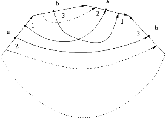
For any fixed , let be any vector field on such that the Euler class of the -plane bundle is Poincaré dual to , where is a curve in that projects to the dotted curve in Figure 9. Let be any knot in that projects to the solid curve in Figure 9. We assume that is perturbed slightly so it is -transverse. This does not determine a unique -transverse isotopy class, but that is not a problem. Let be the connected component of the space of framed immersions containing . Let be any other -transverse knot in .
9.1 Lemma ([5] proof of Lemma 6.11).
Let . Then contains a representative of the form .
Proof. Pick a representative . Since is a loop in the space of immersions, we can lift to a loop also called where is the lift of to the spherical tangent bundle . Now we regard as a map and consider the possible values of , the trace of the basepoint of in . For the precise definition of see Section 12. The image of is the centralizer of . From the long exact sequence of the bundle , and from the fact that the centralizer of is the cyclic subgroup generated by , we conclude that any element of the centralizer of in is of the form where is the class of the -fiber. On the other hand, and , so by Proposition 12.2, is homotopic to a representative of the form . ∎
For the next Lemma, we introduce an invariant of knots in . Let be a singular knot with one double point at and view as a pair of maps . Let if both are noncontratible and let otherwise. We say a loop or path is generic if, whenever is a singular knot, has exactly one transverse double point and no other multiple points, and the set of times such that is singular is a discrete set . In particular any loop in has a generic representative.
A transverse double point of a singular knot can be resolved in two different ways. We say that a resolution of a double point is positive (resp. negative) if the tangent vector to the first strand, the tangent vector to the second strand, and the vector from the second strand to the first form a positive -frame. This does not depend on the order of the strands.
We assign a sign to each singular knot as follows: if, for , is obtained from the singular knot by a positive resolution of its double point, put . Otherwise .
For any generic define .
The set of singular knots forms the discriminant in The codimension two (with respect to ) stratum of the discriminant consists of singular knots with two distinct transverse double points. It is easy to see that , for every small generic loop going around the codimension two stratum. This implies (cf. Arnold [1]) that if is a generic loop in that starts at a nonsingular knot , then depends only on the element of realized by a generic loop .
9.2 Lemma.
The value of the invariant on is . In particular, no element of the homotopy class is represented by a self-isotopy of , that is, an element of .
Proof. Clearly for any which is homotopic to a loop in . However . The knot crosses the fiber over the self-intersection point of twice. During the homotopy , these two points move along the fiber at unit speed in opposite directions because the two loops in one gets by smoothing at are orientation reversing. Therefore is singular at two times and , and because and are equal and . The last identity holds because the two loops adjacent to a double point of singular knots project to orientation reversing loops on and hence are not contractible in Hence is not homotopic to a loop in .∎
9.3 Lemma.
Let be any knot homotopic to through immersed curves, where is a knot projecting to . Let . If is represented by a self-isotopy of , that is, an element of , then contains a representative of the form for some integers and .
9.4 Remark.
Note that one can show that , but we will not need this stronger version of the lemma.
Proof. Choose a homotopy from to in , and write with . Thus . By Lemma 9.1, we may write . Now . By Lemma 9.2, . Since is homotopic to an isotopy, . Lastly, since the singular knot which appears during can be viewed as an ordered pair of two loops, at least one of which is contractible. For to be homotopic to an isotopy we must have . Thus , so while thus far and can be any integer. Now and . But is homotopic to , where is now viewed as a rotation of the parametrizing circle of rather than and is the homotopy which passes through a small kink of rather than . Note that the loop is a framed isotopy, while the loop is not even an isotopy.
∎
9.5 Theorem.
Let be the oriented total space of an -bundle over a non-orientable surface of genus and let be the solid curve pictured in Figure 9. Let be any homotopy class of framed immersions containing a framed knot that projects to For each there exists a nowhere-zero vector field on such that no knot type in is simple. In particular, for any -transverse knot in , the -transverse knots and are homotopic through -transverse immersions, isotopic as framed knots, and not isotopic through -transverse knots.
Proof. Let be a vector field on such that the Euler class of the -plane bundle on is Poincaré dual to the class where is some curve in projecting to the dotted curve in Figure 9. The fact that such a vector field exists follows, for example, from the Pontryagin-Thom Construction, see for example Section 8. Furthermore, choose so that it intersects the fiber over transversely in one point, and is disjoint from .
To simplify notation in the remainder of the proof, we write rather than .
We begin by showing that the knot type of is simple.
We claim that . To show this, we must find a framed self-homotopy such that . Let . The lift of intersects transversely in one point. Since is Poincaré dual to , we have .
Now we must show that . It suffices to show . Suppose and . We may apply Lemma 9.3, and use the lemma in the case where . We conclude that is represented by the loop for some integers and . But since the corresponding torus is disjoint from , contradicting our assumption.
Now we will show that any knot type in is simple. Let be any knot homotopic to through framed immersions. We first check that . (Now the homomorphisms are viewed as maps using basepoint , and the homomorphism is a map from , where is the connected component of the space of framed knots containing ) Again let , where now is the framed self-homotopy of given by sliding around the fiber. Let be any path from to in . We can write , where is the self-homotopy of given by sliding around the fiber. Now as desired.
Last we show , and as before it suffices to show that . Suppose , where is the isotopy class of , and . We may apply Lemma 9.3, and conclude that contains a representative of the from . Again this is disjoint from so , contradicting our assumpton. ∎
The knots in Theorem 9.5 can be chosen to be Legendrian with an overtwisted complement. This is because the result of Eliashberg [12] says that every -plane distribution in is homotopic to an overtwisted contact structure. We make this precise in the following corollary.
9.6 Corollary.
Let be an oriented 3-manifold as in Theorem 9.5 with a cooriented contact structure homotopic to the 2-plane field . For each framed knot type containing a Legendrian representative , the stabilized Legendrian knots and are isotopic as framed knots, and homotopic as Legendrian immersions, but not isotopic as Legendrian knots; these Legendrian knots can be chosen to be loose.
Proof.
Let be a Legendrian curve which projects to the knot in 9.5. It is straightforward to check that and are isotopic as framed knots. Recall from the introduction that is isotopic to through -transverse (in this case, pseudo-Legendrian) knots. By Theorem 9.5, and are homotopic through -transverse immersions, but not isotopic through -transverse knots. Hence the same is true of and . By the -principle for Legendrian immersions [17] (see Theorem 12.3), and are homotopic as Legendrian immersed curves. The corollary follows. ∎
10. Homotopy classes containing Simple and Nonsimple Knot Types
In this section we construct framed knot types and with homotopic representatives ( for some component of the space of framed curves), such that is simple while is not. This is in contrast to the example in the last section, where we described a homotopy class in which all knot types were nonsimple.
Let be an -bundle over an oriented surface of genus . Let be any curve in projecting to the solid loop pictured in Figure 10 to and let be a vector field on such that is Poincaré dual to . Let be a vertical fiber with some framing.
Let be a framed knot obtained from by pulling a small arc of around a loop in which projects to a loop freely homotopic to on and then passing through a double point, see Figure 11. The loop is pictured in Figures 10.
Let denote the component of the space of immersions containing and . Now we characterize all possible self-homotopies of . Recall that the definition of can be found in Subsection 7.5.
10.1 Lemma ([5] proof of Lemma 6.11).
Let . Then contains a representative of the form for some choice of , where .
Proof. The proof is similar to that of Lemma 9.1. Again the trace of the basepoint under a self homotopy commutes with the curve . In this case, the trace of the basepoint of must commute with the class of the fiber . But is in the center of , so can be any element of . In particular we may write for some loop which projects to . But for some choice of loop , the loop has trace as well. Now the lemma follows from Proposition 12.2.∎
10.2 Proposition.
Let be a path from to which unclasps and is an isotopy at all other times. Every loop in has a representative of the form for some .
Proof. This follows directly from Lemma 10.1.∎
10.3 Definition (Schneiderman’s invariant).
Now we recall an invariant due to Schneiderman [20] which we use in the proof of the next lemma. Let be a -manifold and let be a properly immersed annulus. Let be a basepoint of and let be a basepoint of . A whisker for is a choice of path from to ; fix some whisker . For each self-intersection point of , the sheets at are the two transversely intersecting immersed -disks in a small neighborhood of in . For each self-intersection define a loop as follows: go along to , go along a path in to , switch sheets, return to without passing through any other double points of , and then return to along . The loop is well defined up to powers the loop where . Define a sign by comparing the orientation of at with the orientation given by the two sheets of at . Now
Let where denotes the free abelian group generated by the elements of . Note that if one wants an invariant of homotopy rather than just regular homotopy one should add to the denominator of the quotient; for our purposes a regular homotopy invariant is enough.
Following Wall [24], Schneiderman [20, Proposition 4.1.2] proves that , when viewed as an element of the quotient , is an invariant of regular homotopy, and whenever vanishes on , the double points of can be paired off with Whitney disks. In higher dimensions, because of the Whitney trick, vanishes if and only if is regularly homotopic to an embedding; in dimension , vanishing is just a necessary condition for to be regularly homotopic to an embedding.
10.4 Lemma.
The class is not represented by an element of if for some .
Proof. Let and be the preimages of the double point of the singular knot which appears during the homotopy at time ; that is, for some . We assume that this unclasping homotopy has the properties that , and for . The loop is pictured in Figure 10.
By modifying our choice of loop , we may assume . Also, commutes with and , so we begin by considering .
We consider the track of the homotopy in . By this we mean, consider the following map :
If the loop is homotopic to a loop in , then the immersed annulus is homotopic to an embedded one, through maps fixing the boundary. We compute and conclude that if does not commute with in , then is not homotopic to an embedded annulus.
Now we compute the two terms of corresponding to the times and at which the self-homotopy of is singular. For our purposes it will actually be enough to compute the projections of the terms of to .
The projection to of the term of corresponding to the first singular time is
A picture of this loop in can be found in Figure 13.
Now we consider the projection to of the term of corresponding to the second singular time .
The projection to of the term of corresponding to the second singular time is
Since , and for , we have
and
Thus
Now we check whether the two terms and are equal in the quotient , where . Since is homotopic to the fiber, It follows that these two terms of do not cancel unless and commute in . Since centralizers in the fundamental group are infinite cyclic, and since is not a nontrival power of another loop, and commute if and only if for some .∎
10.5 Theorem.
Let be an -bundle over an orientable surface of genus . Let be the framed homotopy class of the fiber with any framing. Then for any there exists a nowhere-zero vector field such that the knot type of is simple in while the knot type of is not. In particular, the knots and are homotopic through -transverse immersions, isotopic as framed knots, and not isotopic through -transverse knots.
Proof. In this proof, we write rather than to simplify notation.
First we consider the knot type of . The loop is a framed self-homotopy and a framed self-isotopy of . The corresponding torus intersects once transversely. Therefore , so and . Furthermore is the smallest positive integer in or , since any such torus intersects at least once or not at all. This and the knot type is simple by Corollary 4.8.
Now we consider the knot type of . In this case the loop is a framed self-homotopy of so as before . Let be an arbitrary framed self-isotopy of . By Proposition 10.2 we know is represented by a loop of the form for some . By Lemma 10.4, since is a framed self-isotopy, for some . But is disjoint from , so . Hence , and the knot type of is not simple. In particular Lemmas 4.4 and 4.5 imply and are homotopic through -transverse immersions and not isotopic as -transverse knots. ∎
As in Theorem 9.5, the knots in Theorem 10.5 can be chosen to be Legendrian with an overtwisted complement. The proof of Corollary 10.6 is similar to the proof of Corollary 9.6.
10.6 Corollary.
Let be an oriented 3-manifold as in Theorem 10.5, with a cooriented contact structure homotopic to the 2-plane field . Let be a Legendrian knot which is smoothly isotopic to the knot in Theorem 10.5. Then the stabilized Legendrian knots and are isotopic as framed knots, and homotopic as Legendrian immersions, but not isotopic as Legendrian knots; these Legendrian knots can be chosen to be loose.
11. Applications to Legendrian Knot Theory
A Legendrian knot in an overtwisted contact -manifold is called loose if where is an overtwisted disk. In many situations, loose Legendrian knots are completely determined by classical invariants. Dymara [10, Theorem 4.1] showed this is true, for example, when is trivializable and . Ding and Geiges [8] generalized Dymara’s result to the case where the connected component of the space of immersions containing contains infinitely many components of the space of Legendrian knots, and again .
Our theory leads to a classification of loose Legendrian knots in terms of generalized classical invariants which generalizes the results of Dymara and Ding-Geiges. We use an -principle stated by Cieliebak and Eliashberg, and attributed to Dymara [10] and Eliashberg-Fraser [14].
-principles for Legendrian knots
We recall some terminology from Cieliebak and Eliashberg [7], using their notation. If and are manifolds, a monomorphism is a bundle map which is injective on each fiber. For example, given an immersion , the differential is a monomorphism .
Now let be a contact -manifold and a manifold of dimension . In our case and . A formal Legendrian embedding is a pair consisting of a smooth embedding and a homotopy of monomorphisms over starting at and ending at an isotropic or Legendrian monomorphism, meaning lies in .
Two formal Legendrian embeddings are called formally isotopic if they are isotopic as (connected by a path of) formal Legendrian embeddings.
11.1 Theorem ([7]Theorem 7.19 b).
Let be a closed connected overtwisted contact -manifold and an overtwisted disk.
Let , be a formal Legendrian isotopy in connecting two genuine Legendrian embeddings . Then there exists a Legendrian isotopy connecting and , which is homotopic to through formal Legendrian isotopies with fixed endpoints.
We use Theorem 11.1 to obtain the following result.
11.2 Theorem.
Let be a closed overtwisted contact manifold with overtwisted disk , and let be the coorienting vector field of . Let and be Legendrian knots in that are -transverse isotopic. Then they are Legendrian isotopic in .
Proof.
Fix an auxiliary Riemannian metric with the property that is everywhere orthogonal to . Let denote the -transverse isotopy from to . That is, for all , is a -transverse knot, and and are Legendrian. We use the -transverse isotopy from to to construct a formal Legendrian isotopy from to . Let denote the normalized orthogonal projection of the tangent vector to the contact plane . Let denote the vector in at the point . Let denote the angle between and its projection . Let
which is a unit vector in . Then is equal to and is tangent to . Hence for each , the pair is a formal Legendrian embedding. Now the theorem follows from Theorem 11.1. ∎
As an application of the above theorem we get the following:
11.3 Theorem.
Let be a closed connected overtwisted contact manifold with overtwisted disk . Let be two loose Legendrian knots in the smooth isotopy class . Assume the following conditions hold:
- (1)
and are isotopic as framed knots (and hence lie in some framed isotopy class )
- (2)
and are homotopic as Legendrian immersions
- (3)
, where is a coorienting vector field for , and and are the kink-cancelling homomorphisms associated to .
Then and are isotopic as Legendrian knots.
Proof.
Below we state theorems of Dymara [10] and Ding-Geiges [8] which we will show follow from Theorem 11.3.
11.4 Theorem ([10], Theorem 4.1).
Let be a contact manifold with an overtwisted disk and a trivializable contact bundle. Let be two loose Legendrian knots in the smooth isotopy class . Assume the following conditions hold:
- (1)
- (2)
and are isotopic as framed knots
- (3)
the rotation numbers of and with respect to some trivialization of are equal.
Then and are isotopic as Legendrian knots.
This theorem of Dymara in the case of closed can be viewed as a special case of Theorem 11.3. This is because when is trivializable, for every framed isotopy class. Note that for trivializable the -transverse homotopy classes of curves in a fixed component of the space of framed curves are enumerated by a -valued rotation number, which is obtained by projecting the velocity vector of a -transverse curve to the planes of .
Ding and Geiges [8, Theorem 6] generalized Dymara’s theorem to the case where is not necessarily trivializable:
11.5 Theorem ([8], Theorem 6).
Let be a closed connected contact manifold with an overtwisted disk . Let be two loose Legendrian knots in the smooth isotopy class . Assume the following conditions hold:
- (1)
- (2)
and are isotopic as framed knots
- (3)
and are homotopic as Legendrian immersions
- (4)
the connected component of the space of framed immersions containing and contains infinitely many components of the space of Legendrian immersions.
Then and are isotopic as Legendrian knots.
As shown in [22, Proposition 3.1.4], the assumption that the connected component of the space of framed immersions contains infinitely many components of the space of Legendrian immersions is equivalent to the following: For any which is realizable by a mapping with meridian freely homotopic to a loop in , we have . Therefore assumption of Ding and Geiges implies that . Thus their theorem is also a special case of Theorem 11.3.
Ding and Geiges [8, Remark, p. 121] remark that conditions and of their theorem are necessary unless one makes certain ad-hoc assumptions about and .
It is possible to coarsely classify zero-homologous loose knots even when two such knots do not have the same overtwisted disk in their complement. The following classification of loose knots up to contactomorphism was given in the work of Etnyre [15, Theorem 1.4]. (According to [15] different proofs of this result were independently obtained by Geiges and Klukas.) Zero-homologous framed knots corresponding to a given unframed knot are enumerated by the self-linking number, which is the Thurston-Bennequin invariant of a Legendrian knot with the natural framing; and the sum of the and of a Legendrian knot is always odd.
11.6 Theorem ([15], Theorem 1.4).
Let be an overtwisted contact manifold. For each zero-homologous knot type and a pair of integers such that is odd, there is a unique, up to contactomorphism, loose Legendrian knot in satsifying and
12. Appendix: -principles
-principle for immersed curves
We will use an -principle in order to understand the topology of a component of the space of framed immersions of the circle into . Let be the unit two-sphere tangent bundle over .
12.1 Theorem (Hirsch-Smale -principle, [17]; see also Theorem 7.1 of [7]).
Let be a -manifold. The space of immersed curves in is weak homotopy equivalent to the space of continuous free loops in . The weak homotopy equivalence is given by mapping the immersed curve to the loop , where , .
Let , with . Then can also be viewed as a map defined by . Identify with the unit circle in . Let be the loop in traced by the basepoint during the homotopy .
The map is in fact a homomorphism . The image of is precisely the centralizer . Now we consider its kernel. Suppose that . Then the -skeleta and are homotopic in ; in fact, they agree on . The obstruction to and being homotopic is therefore the element of formed by gluing the two -cells in the images of and together along their common -skeleta. Note that is trivial, so we choose an identification , which gives an isomorphism . In addition, we can identify with and view as a map into when convenient.
In our case, will be an -bundle over a surface of genus at least , so .
12.2 Proposition ([5]).
Let be an oriented -manifold with , let be a connected component of the space of immersed curves in , and let be a knot. Let such that . Then where is the first coordinate in .
h-principle for Legendrian immersions
12.3 Theorem (Gromov [17]).
Let be an oriented 3-manifold with cooriented contact structure , and let denote the corresponding sphere bundle. The space of Legendrian immersions of into is weak homotopy equivalent to the space of continuous free loops in . The weak homotopy equivalence is given by mapping the Legendrian immersion to the loop , where , .
Acknowledgments. This paper was written when the authors were at Max Planck Institute for Mathematics, Bonn and the authors thank the institute for its hospitality. This work was partially supported by a grant from the Simons Foundation to Vladimir Chernov and to Patricia Cahn.
The authors are thankful to Stefan Nemirovski and Spiridon Adams-Florou for enlightening discussions. The authors are grateful to the anonymous referee for all the valuable comments and suggestions.
References
- [1] V. I. Arnold Plane curves, their invariants, perestroikas and classifications, Singularities and Bifurcations (V.I. Arnold, ed.) Adv. Sov. Math. vol. 21, (1994), pp. 39–91
- [2] R. Benedetti, C. Petronio Combed 3-manifolds with concave boundary, framed links, and pseudo-Legendrian links, J. Knot Theory Ramifications 10 (2001), no. 1, 1–35.
- [3] R. Benedetti, C. Petronio Reidemeister-Turaev torsion of 3-dimensional Euler structures with simple boundary tangency and pseudo-Legendrian knots, Manuscripta Math. 106 (2001), no. 1, 13–61
- [4] P. Cahn, V. Chernov, R. Sadykov The number of framings of a knot in a -manifold preprint arXiv:1404.5851 (2014) 8 pages
- [5] V. Chernov Framed knots in 3-manifolds and affine self-linking numbers, J. Knot Theory Ramifications 14 (2005), no. 6, 791–818
- [6] V. Chernov Relative framing of transverse knots, Int. Math. Res. Not. (2004) no. 52, 2773–2795
- [7] K. Cieliebak Ya. Eliashberg From Stein to Weinstein and Back Symplectic Geometry of Affine Complex Manifolds a book available at http://www.mathematik.uni-muenchen.de/ kai/research/stein.pdf 372 pages
- [8] F. Ding and H. Geiges Handle moves in contact surgery diagrams, J. Topology 2, no. 1, pp. 105–122 (2009).
- [9] M. do Carmo Riemannian geometry. Mathematics: Theory & Applications. Birkäuser Boston, Inc., Boston, MA (1992)
- [10] K. Dymara Legendrian knots in overtwisted contact structures on Ann. Global Anal. Geom. 19, no. 3, 293–305 (2001)
- [11] K. Dymara Legendrian knots in overtwisted contact structures http://arxiv.org/abs/math/0410122 (2004) 34 pages
- [12] Ya. Eliashberg Classification of overtwisted contact structures on 3-manifolds Invent. Math. 98 (1989), no. 3, 623–637
- [13] Ya. Eliashberg Contact -manifolds twenty years since J. Martinet’s work, Ann. Inst. Fourier (Grenoble) 42 no. 1-2 (1992), pp. 165–192
- [14] Ya. Eliashberg and M. Fraser Topologically trivial Legendrian knots J. Symp. Geom. 7 no. 2, 77–127 (2009).
- [15] J. Etnyre On knots in overtwisted contact structures Quantum Topol. 4 (2013), no. 3, 229–264
- [16] H. Geiges An introduction to contact topology. Cambridge Studies in Advanced Mathematics, 109 Cambridge University Press, Cambridge (2008)
- [17] M. Gromov Partial Differential Relations, Springer, Berlin, Heidelberg, 1986.
- [18] R. Lutz Structures de contact sur les fibrés principaux en cercles de dimension , Ann. Inst. Fourier, 3 (1977), pp. 1–15
- [19] D. McCullough Homeomorphisms which are Dehn twists on the boundary, Algebr. Geom. Topol., Vol 6 (2006), pp. 1331–1340.
- [20] R. Schneiderman. Algebraic linking numbers of knots in 3-manifolds, Algebr. Geom. Topol. 3 (2003), pp. 921–968.
- [21] V. Tchernov (Chernov). Isomorphism of the groups of Vassiliev invariants of Legendrian and pseudo-Legendrian knots, Compositio Math. 135 (2003), no. 1, 103–122
- [22] V. Tchernov (Chernov). Vassiliev invariants of Legendrian, transverse, and framed knots in contact three-manifolds, Topology 42 (2003), no. 1, 1–33
- [23] B. Trace. On the Reidemeister Moves of a Classical Knot, Proc. Amer. Math. Soc. 89 (1983), no. 4, 722–724.
- [24] C. T. C. Wall. Surgery on Compact Manifolds. London Math. Soc. Mono- graphs 1, Academic Press, (1970) or Second Edition, edited by A. Ranicki, Math. Surveys and Monographs 69, A.M.S.