Bargaining-based Mobile Data Offloading
Abstract
The unprecedented growth of mobile data traffic challenges the performance and economic viability of today’s cellular networks, and calls for novel network architectures and communication solutions. Data offloading through third-party WiFi or femtocell access points (APs) can effectively alleviate the cellular network congestion in a low operational and capital expenditure. This solution requires the cooperation and agreement of mobile cellular network operators (MNOs) and AP owners (APOs). In this paper, we model and analyze the interaction among one MNO and multiple APOs (for the amount of MNO’s offloading data and the respective APOs’ compensations) by using the Nash bargaining theory. Specifically, we introduce a one-to-many bargaining game among the MNO and APOs, and analyze the bargaining solution (game equilibrium) systematically under two different bargaining protocols: (i) sequential bargaining, where the MNO bargains with APOs sequentially, with one APO at a time, in a given order, and (ii) concurrent bargaining, where the MNO bargains with all APOs concurrently. We quantify the benefits for APOs when bargaining sequentially and earlier with the MNO, and the losses for APOs when bargaining concurrently with the MNO. We further study the group bargaining scenario where multiple APOs form a group bargaining with the MNO jointly, and quantify the benefits for APOs when forming such a group. Interesting, our analysis indicates that grouping of APOs not only benefits the APOs in the group, but may also benefit some APOs not in the group. Our results shed light on the economic aspects and the possible outcomes of the MNO/APOs interactions, and can be used as a roadmap for designing policies for this promising data offloading solution.
Index Terms:
Mobile Data Offloading, Nash Bargaining Solution, Group BargainingI Introduction
I-A Background and Motivations
The global mobile data traffic is growing explosively, and it is expected that by 2018, it will reach exabytes per month, nearly an -fold increase over 2013 [1]. To cope with this unprecedented traffic load, mobile network operators (MNOs) need to significantly increase their cellular network capacities. However, traditional methods such as acquiring more spectrum licenses, deploying new cells of small size, and upgrading technologies (e.g., from WCDMA to LTE/LTE-A) are costly, time-consuming, and may not catch up the pace of the traffic increase. Clearly, MNOs must find novel methods to address this problem, and mobile data offloading appears as one of the most attractive solutions.
Simply speaking, mobile data offloading is the use of complementary network technologies (such as WiFi and femtocell) for delivering the mobile data traffic originally targeted for cellular networks. The performance benefit of data offloading through WiFi and femtocell networks has been extensively studied in the existing literature (see, e.g., [9, 10, 11, 12, 13, 15, 14]). Thus, it is not surprising that MNOs want more initiative in determining whether, when, and how much to offload their cellular traffic.11 1 As demonstrations, MNOs have already deployed their own WiFi networks (e.g. AT&T [2]), or initiated collaborations with existing WiFi networks (as O2 did with BT [3]), to complement their cellular networks. Some MNOs have also started offering transparent cellular-WiFi services [4]. This network-initiated offloading approach is greatly facilitated by technological advances such as the Hotspot 2.0 protocol [5], and the 3GPP Access Network Discovery and Selection Function (ANDSF) standard. In order to fully reap these benefits, it is essential to ensure that MNOs are able to offload their traffic whenever needed. To achieve this goal, a high coverage of WiFi or femtocell networks is necessary. Unfortunately, the densely or ubiquitous deployment of WiFi or femtocell access points (APs) by the MNOs themselves is costly and often impractical due to the limitations of additional site spaces and backhauls.
An alternative option for the MNOs is to employ existing WiFi and femtocell APs already deployed by third-parties (as O2 did with BT [3]), instead of deploying their own offloading networks. This novel network outsourcing method is attractive due to the high population of WiFi or femtocell users [6] as well as the technology innovations (e.g., Hotspot 2.0 protocol and 3GPP ANDSF standard) enabling such a cellular-WiFi inter-networking. With this approach, MNOs can handle data offloading with a reduced capital expenditure (CAPEX) and operational expenditure (OPEX). Moreover, MNOs can make the offloading decisions more flexibly and efficiently, by employing APs on-demand taking into consideration the traffic dynamics. Nevertheless, without proper incentives, the APs’ owners (APOs) are expected to be reluctant to admit the cellular traffic, since offloading cellular traffic will consume their limited network capacities and increase various costs such as the energy expenditure and the backhaul cost. This important economic incentive issue, however, is still quite under-explored in the existing literature.
I-B Contributions
In this paper, we study the mobile data offloading via third-party WiFi and femtocell APs, and focus on the necessary economic incentives that MNOs need to provide for APOs in order to achieve flexible on-demand data offloading. Specifically, we consider such an offloading scenario, where one MNO offloads its cellular traffic to a set of third-party WiFi or femtocell APs. The MNO serves its subscribed mobile users (MUs) in one or multiple macrocells. Each AP can only offload the traffic generated by (cellular) MUs within its coverage. Figure 1 illustrates such a network scenario, where the hexagons denote the coverage areas of the MNO’s macrocells, and the blue circles denote the much smaller (non-overlapping) coverage areas of APs. In this example, the traffic of MUs 1 and 2 can be offloaded to AP 1, and the traffic of MU 7 can be offloaded to AP 5, while the rest MUs cannot take advantage of offloading, as they are not within the coverage area of any AP. In such an offloading model, we are interested in the following technical and economical issues:
- •
Technical issue: How to offload traffic efficiently (i.e., maximizing the social welfare)?
- •
Economical issue: How to share the offloading benefit among the MNO and APOs fairly?
Note that the second (economical) issue is particularly important as it is closely related to the incentives of APOs. More specifically, to address these issues, we need to answer the following offloading and reimbursing problem explicitly: (i) For the MNO, how much traffic should it offload to each AP and how much pay each APO? and (ii) For each APO, how much cellular traffic should it offload for the MNO and how much charge to the MNO? Clearly, the successful deployment of such a cooperative offloading architecture requires the MNO and APOs to agree on both the offloading amount and the payment. One proper theoretic framework to achieve this goal is the cooperative game theory.22 2 Game theory [34] is widely used in wireless networks to model interactions of multiple network entities, where the actions of one entity (player) affect the payoffs of the other entities (see, e.g., [37, 38, 36, 35, 39]). Cooperative game theory is usually used in situations when players have conflicting/competing interests but have the means (and also incentives) to coordinate and negotiate with each other to achieve a mutually beneficial outcome. In our model, it is natural to assume that the MNO and APOs can get in touch and coordinate regarding offloading and reimbursing decisions. It is then natural to study the data offloading problem using the cooperative game theory.

In this work, we model and analyze the data offloading problem by using the Nash bargaining theory [24], a special branch of the cooperative game theory, which is expected to yield a Pareto-efficient and fair outcome, hence self-enforcing and satisfactory for all entities. In this bargaining model, the MNO negotiates with each APO for the amount of offloading data and the respective payment. We formulate the entire negotiation processes between the MNO and all APOs as a one-to-many bargaining game, and study the game outcome (bargaining solution) systematically. There are many challenging issues arising in a one-to-many bargaining.
Bargaining Protocol. An important issue arising naturally in a one-to-many bargaining is the bargaining dynamics (called bargaining protocol), namely, how the MNO bargaining with multiple APOs, e.g., sequentially or concurrently? In this work, we will study two different bargaining protocols systematically: (i) sequential bargaining, where the MNO bargains with all APOs sequentially in a predefined order, and (ii) concurrent bargaining, where the MNO bargains with all APOs concurrently. There are many interesting open questions associated with this bargaining protocol. For example, will an APO gain certain benefit if it bargains with the MNO ahead of other APOs (in the sequential bargaining)? How would the MNO choose between sequential or concurrent bargaining with multiple APOs? Although the study of bargaining theory is an active research area in economics, there is not much work analyzing this protocol comprehensively.
Grouping Effect. Another important issue in a one-to-many bargaining is the possibility that APOs may form groups (or larger communities) and bargain jointly with the MNO. This allows individual APOs, who initially have less bargaining power than the MNO and may only have limited choices (e.g., accept or reject the terms of the MNO), to gain more market power from the larger collective coverage. Such groups can be created within WiFi sharing communities such as FON [7], or in the context of community networks [8]. Motivated by this, we would like to understand the impacts of the size and the structure of APO groups on the bargaining outcome.
The main contributions are are summarized as follows.
- •
To the best of our knowledge, this is the first paper modeling and studying mobile data offloading using a one-to-many bargaining framework, which yields a fair, Pareto-efficient, and self-enforcing offloading solution.
- •
We characterize the outcome of the one-to-many bargaining under different bargaining protocols and grouping structures, which has not yet been considered completely in the existing literature of Nash bargaining.
- •
We study the impact of the bargaining protocol on the bargaining outcome comprehensively. We quantify the benefits for APOs when bargaining sequentially and earlier with the MNO (early-mover advantage), and the losses of APOs when bargaining concurrently with the MNO (concurrent moving tragedy).
- •
We study the grouping effect on the bargaining solution systematically. Interesting, our analysis indicates that grouping APOs not only benefits the APOs in the group (intra-grouping benefit), but may also benefit some APOs not in the group (inter-grouping benefit).
II Literature Review
II-A Mobile Data Offloading
The performance benefit of mobile data offloading through WiFi networks has been studied in [9, 10, 11, 12, 13], which showed that in urban environments, WiFi can offload about 65% of mobile data, and save 55% of MUs’ battery energy. These benefits can be further enlarged if users are willing to delay their traffic [14]. Another promising option for data offloading is femtocell [15]. The problem of incentivizing femtocell owners to admit macrocell traffic has been recently studied in [16, 17, 18, 19, 20]. However, these works studied the incentive issues using the non-cooperative game framework, which cannot capture the potential of coordination among mobile operators and femtocell owners (which calls for a cooperative game approach). In [21], Zhang et. al. studied the economic incentive issue by using the cooperative game framework (Nash bargaining) as we did in this work. However, the bargaining model in [21] is the simple one-to-one bargaining (between one mobile operator and one fixed-line operator), while the bargaining model in our work is a more general one-to-many bargaining (between one MNO and many APOs).
In our previous works, we have studied the economic incentive issue in mobile data offloading via third-party APs, by using either the non-cooperative Stackelberg game framework [22] or the auction framework [23]. However, these works can neither capture the potential of coordination among the MNOs and APOs, nor the effect of market dynamics (e.g., the bargaining protocol in our model) or user collusions (e.g., the grouping of APOs in our model).
II-B Nash Bargaining Theory
Nash in [24] established a basic two-person bargaining framework between two rational players, and proposed an axiomatic solution concept—Nash Bargaining Solution (NBS), which is characterized by a set of pre-defined axioms (see Section IV-A), and does not rely on the detailed bargaining process of players. In the follow up work, Nash [25] and Rubinstein [26] provided strategic foundations for the NBS, by analyzing specific dynamic non-cooperative bargaining processes (games) and showing that the equilibria of the bargaining games converges to the NBS.
Since Nash’s pioneering work, researchers have extended the bargaining analysis to the case of more than two players. In the multi-player scenario, some players may form groups and bargain jointly in order to improve their payoff (hence the group bargaining [27]). In most cases, the grouping improves the payoff of the group members (see [28, 29, 30]), as it increases their collective bargaining power. Interestingly, the opposite is also possible as shown by the Harsanyi bargaining paradox [31]. However, the above works did not consider the bargaining dynamics (bargaining protocol) among multiple bargainers, which arises naturally in a multi-player bargaining. Regarding the bargaining protocol, the most relevant models are those in [32, 33]. However, both papers focused only on the sequential bargaining, using either an axiomatic approach [32] or a strategic approach [33], and neither considered the concurrent bargaining, nor the grouping effect.
III System Model
III-A System Description
We consider one mobile network operator (MNO), operating one or multiple macrocells, wants to offload its cellular traffic to a set of third-party WiFi or femtocell access points (APs).33 3 In this work, we do not distinguish WiFi APs and femtocell APs, as we will model APs using generic objective (cost) functions. This renders our analysis appropriate for a variety of systems with various assumptions. We assume that the coverage areas of any two APs are non-overlapping. This assumption is reasonable as the transmission range of AP is much smaller than that of the macrocell base station (BS).44 4 In our online technical report [40], we also discuss how to extend the current model to a more general model with overlapping APOs. Figure 1 illustrates such a network with non-overlapping APs and macrocell BS.
The MNO serves a set of macrocell mobile users (MUs) who are randomly distributed in geography. The traffic generated by an MU can be offloaded to an AP, if the following conditions are all satisfied:
- •
The MU is located within the coverage area of the AP (hence attainable for the AP),
- •
The MU is equipped with the same radio frequency interface and wireless communication protocol as the AP (hence compatible with the AP),
- •
The MU is enabled to offload its traffic (e.g., WiFi is turned on for offloading to a WiFi AP).
Let denote the set of MUs whose traffic can be offloaded to AP , and denote the set of MUs whose traffic cannot be offloaded to any AP. As the APs’ coverage areas are non-overlapping, we have: with . In the example of Figure 1, the traffic of MUs 1 and 2 can be offloaded to AP 1 and the traffic of MU 7 can be offloaded to AP 5 (supposing these MUs are compatible with APs and enable WiFi), while the traffic of MUs 3-6 cannot be offloaded to any AP.
Let denote the total cellular traffic that can be offloaded to AP (i.e., the total traffic generated by MUs in ), and denote the total cellular traffic that cannot be offloaded to any AP (i.e., the total traffic generated by MUs in ). The traffic profile of the MNO is denoted by
Due to the uncertainty of MUs’ mobility and data usage, the value of for each changes randomly over time. We consider a quasi-static network scenario, where the values of for all remain unchanged within every data offloading period (e.g., one minute in our simulation).55 5 Note that when considering the large times-scale bargaining period (e.g., when the bargaining is performed every hour or every day), and will correspond to the estimations of the average traffic.
We define the transmission efficiency of a communication link (between an MU and its attached macrocell BS, or between an MU and an AP) as the average amount of data traffic (in bits) that can be delivered by one unit of spectrum resource (in Hz) per time unit (in second). Obviously, the transmission efficiency is closely related to the path loss and shadow fading of a link. As a concrete example, we can compute it based on the Shannon channel capacity. But our discussions are general for any choice of transmission efficiencies in different communication systems.
Let denote the average transmission efficiency (in bits/Hz/s) between MUs in (in AP ’s coverage area) and their corresponding macrocell BS, and denote the average transmission efficiency between MUs in (not in any AP’s coverage area) and their corresponding macrocell BS. That is, delivering one unit of traffic generated by (or ) within a single time unit, on average, consumes (or ) units of the MNO’s resource. The transmission efficiency profile of the MNO is denoted by
Let denote the average transmission efficiency between MUs in and AP . That is, offloading one unit of cellular traffic generated by within a single time unit, on average, consumes units of AP ’s resource. The transmission efficiency profile of APs is denoted by
We similarly assume that and remain unchanged within every offloading period, but may changes across periods. Our analysis focus on the offloading solution in a single period.
III-B MNO Modeling
We focus on the direct benefit for the MNO from data offloading, i.e., the serving cost reduction due to the reduced resource consumption.66 6 Some indirect benefits include (i) the improvement of MUs’ QoS and thus the increase of the average revenue per user (ARPU), (ii) the increased number of active MUs and thus the increased total revenue, and (iii) the reduction of the network congestion and thus the saving of the MNO’s reputation. Such a serving cost may include the energy cost, operational cost, coordinating cost, etc. Let denote the MNO’s serving cost for units of resource consumption. We will consider a generic cost function that is continuous, differentiable, strictly increasing, and convex, i.e., and .
Let denote the traffic offloaded to AP , and denote the MNO’s payment to the owner of AP (denoted by APO ). The traffic offloading profile and payment profile are, respectively,
Given and , the MNO’s total resource consumption for delivering remaining un-offloaded traffic is
| (1) |
and the MNO’s total cost, including both the serving cost and the payment to APOs, is
| (2) |
The MNO’s payoff is defined as the total cost reduction achieved from data offloading, denoted by
| (3) | ||||
where , and is the MNO’s serving cost reduction. We refer to the MNO’s payoff without data offloading as its reservation payoff, denoted by . As we will show later, this reservation payoff serves as the disagreement point of the MNO, and plays an important role in the bargaining.
III-C APO Modeling
Each AP is owned by a private owner (APO), whose primary goal is to serve its own users. Thus, each APO, when deciding whether (and how, if so) to offload traffic for the MNO, must take into consideration the demand of its own users.
Let denote the APO ’s own resource demand (from its own users). Due to the uncertainty of AP users’ mobility and data usage, we define as a random variable, falling within a certain interval and following a probability distribution function (PDF) and a cumulative distribution function (CDF) . We assume that , are independent of each other, but not necessarily identically distributed. Let denote the total resource owned by APO . Let denote the average revenue achieved from one unit of its own resource demand, and denote the cost for one unit of its resource consumption. Then, APO ’s expected profit (from serving its own demand) is
| (4) | ||||
Recall that the average transmission efficiency between AP and MUs in is . If AP admits units of cellular traffic (generated by MUs in ), the total resource consumption for the offloaded cellular traffic is , and thus the resource left for serving its own demand is . Obviously, a feasible must satisfy: . Given feasible and , the APO ’s total profit, including both the profit from serving its own demand and the profit from offloading for the MNO, is
| (5) |
where is the profit from helping the MNO, consisting of the service income (i.e., the MNO’s payment) and the serving cost.
The APO ’s payoff is the profit improvement when offloading traffic for the MNO, denoted by
| (6) | ||||
where is the APO ’s profit loss induced by data offloading. Similarly, we refer to the APO ’s payoff when not offloading traffic for the MNO as its reservation payoff, denoted by . This reservation payoff serves as the disagreement point of APO in the bargaining.
III-D Social Welfare
The social welfare is defined as the aggregate payoff of the MNO and all APOs, denoted by
| (7) | ||||
That is, the social welfare is equivalent to the sum of the MNO’s serving cost reduction and the APOs’ profit loss, as the payments will be canceled out. Thus, we will also write the social welfare as .
IV A Simple One-to-One Bargaining
In this section, we first review the Nash bargaining theory. Then we consider a simple model with one APO, and formulate the problem as a basic two-person one-to-one bargaining. We use this simple example to illustrate how to formulate and analyze a data offloading problem by using the Nash bargaining framework. This can help us to better understand the bargaining formulation and analysis for general models with multiple APOs in Section V.
IV-A Nash Bargaining Theory
In [24], Nash established the following two-person bargaining framework. There is a set of two players. The players either reach an agreement in a set , or fail to reach agreement, in which case the disagreement event occurs. Each Player has a preference ordering over the set , represented by a utility function over the domain of . We denote such a bargaining problem by . A bargaining solution assigns every bargaining problem an outcome, which can be either an agreement or the disagreement event. Note that an agreement outcome can be either a specific agreement in the set , or a lottery over a set of possible agreements.
Nash proposed four axioms that should be satisfied by a reasonable bargaining solution [24]: Pareto efficiency, symmetry, invariance to affine transformations, and independence of irrelevant alternatives. Nash proved that under mild technical conditions, there is a unique bargaining solution (called Nash bargaining solution, NBS) satisfying the four axioms above. Moreover, the NBS has a very simple form: it corresponds to an outcome that maximizes the product of both players’ utility gains upon the disagreement outcome.
Specifically, let denote the utility of player over the disagreement outcome (i.e., the reservation utility or disagreement point of player ), and denote the set of utility pairs over all possible agreements (i.e., the feasible set). Suppose that (i) is compact (i.e. closed and bounded) and convex, and (ii) there exists an such that .
Definition 1 (Nash Bargaining Solution – NBS [24]).
A pair of utilities (or the associated agreement ) is an NBS (i.e., satisfying Nash’s four axioms), if it solves the following problem:
| (8) | ||||
It is easy to see that the disagreement points and play an important role in the Nash bargaining framework. With a higher disagreement point , player can obtain a larger utility under the NBS.
IV-B One-to-One Bargaining
Now we consider a simple network scenario with one AP. In this case, the bargaining problem is a one-to-one bargaining (one MNO and one APO). For notational consistence, we still denote the APO by , i.e., .
Let and denote the sets of feasible and , respectively. An agreement is a feasible tuple . The agreement set is . The NBS is an agreement that solves the following problem:
| (9) | ||||
Note that in (9), both the MNO and APO have a zero disagreement point, i.e., .
For notational convenience, we introduce a new variable to denote the APO ’s payoff (gain), i.e.,
Then, the MNO’s payoff (gain) can be written as where is the social welfare defined in (7). Substituting the above formulas to (9), we can rewrite (9) as a new optimization problem of and , i.e.,
| (10) | ||||
Note that problems (9) and (10) are equivalent. This implies that the bargaining for is equivalent to the bargaining for . Intuitively, for any bargaining solution on , we can compute an equivalent solution on in the following way: .
It is easy to check that (10) is a convex optimization problem. Thus, we have the following NBS for this simple one-to-one bargaining problem.77 7 We leave all of the detailed proofs in the online technical report [40].
Lemma 1 (One-to-One NBS).
The NBS for the one-to-one bargaining is
where is the social welfare maximization offloading solution.
The above lemma implies that the NBS maximizes the social welfare. Intuitively, this is because the total generated social welfare can be freely transferred between players (through the payment ), and thus maximizing the product of their individual payoff gains can only be achieved when maximizing the overall social welfare. This is a key property the bargaining problem with transferable utility. Note that this phenomena not only exists in a one-to-one bargaining, but also exists in the general one-to-many bargaining studied later.
V One-to-Many Bargaining
In this section, we consider a general model with multiple APOs . In this case, the MNO needs to bargain with every APO for (hence a one-to-one bargaining), and thus the entire bargaining problem becomes a one-to-many bargaining, consisting of coupled one-to-one bargainings. Accordingly, the one-to-many bargaining solution contains agreement or disagreement outcomes, each associated with a one-to-one bargaining (between the MNO and one APO). Clearly, there are two important factors that will affect the outcome of a one-to-many bargaining:
- 1.
Bargaining Protocol: The MNO can either bargain with all APOs sequentially, in a predefined order, or bargain with all APOs concurrently (see Figure 2). We refer to the former one as the sequential bargaining, and the latter one as the concurrent bargaining.
- 2.
APO Grouping Structure: APOs can either bargain individually with the MNO, or form one or multiple groups bargaining with the MNO jointly. An APO group can be exogenously given (e.g., all customers of FON belong to the same group), or endogenously formed based on their instant willingnesses.
In what follows, we will study the bargaining solution of the one-to-many bargaining systematically. We will call it the one-to-many NBS, or just NBS for short. For convenience, we denote the bargaining solution between the MNO and APO as , and the one-to-many NBS as which consists of the bargaining solutions between the MNO and all APOs.
V-A Traffic Offloading Profile under the NBS
We first study the traffic offloading profile under the NBS. Similar to that in the aforementioned one-to-one bargaining, we show that in a general one-to-many bargaining, it still maximizes the social welfare, regardless of the detailed bargaining protocol and the APO grouping structure. Formally,
Lemma 2 (Traffic Offloading Profile).
The traffic offloading profile under the NBS is equivalent to the socially optimal traffic offloading profile .
We present the detailed proof in [40]. Intuitively, our bargaining model is a transferable utility model, and thus the NBS (specifying both the payment transferring and traffic offloading between the MNO and all APOs) always maximizes the social welfare. Besides, the payment transferring is internal and does not affect the social welfare. Therefore, the traffic offloading profile under the NBS must maximize the social welfare. We skip the derivation of the social welfare maximization solution , as it is a standard convex optimization. Readers can refer to the online technical report [40] for details.
V-B Payment Profile under the NBS
Now we study the payment profile under the NBS. As discussed in (9) and (10), the bargaining for (the payments to APOs) is equivalent to the bargaining for (the payoffs of APOs). For the convenience in describing, we will present the NBS in terms of .
In this subsection, we will show that the payment profile or the APO payoff profile greatly depends on the bargaining protocol, and in the next subsection (Section V-C) we will further show that it is also affected by the APO grouping structure. In what follows, we derive the NBS under sequential bargaining (in Section V-B.1) and under concurrent bargaining (in Section V-B.2) systematically.88 8 For better understanding of the analytical bargaining solution, we also provide illustrative examples in the online technical report [40].
B.1) Sequential Bargaining
We first study the NBS under the sequential bargaining, where the MNO bargains with APOs sequentially, in a predefined order (see Figure 2 (a)). Without loss of generality, we assume that the MNO bargains with APOs in the order of . This implies that there is no APO group, i.e., each APO bargains with the MNO individually. The impact of APO grouping will be studied in Section V-C.
Since the underlying one-to-one bargaining problems (between the MNO and each APO) are coupled with each other, we solve the sequential bargaining by backward induction. For the convenience in writing, we introduce notations:
for the analysis of the sequential bargaining.

Step .
Suppose that the MNO has finished bargaining with APOs to , and reached bargaining solutions . Now it bargains with APO for .
1. Disagreement: If the MNO and APO do not reach any agreement, the APO ’s disagreement point is , and the MNO’s disagreement point is its payoff achieved from all prior APOs, i.e.,99 9 Here means with , and the subscript in is used to indicate the stage of bargaining. Later on we will use the same form for notational convenience.
2. Agreement: If they reach an agreement (and ), the payoffs of APO and the MNO are, respectively,
3. Payoff gain: Under an agreement (and ), the payoff gains of APO and the MNO are, respectively,
where denotes the marginal social welfare (i.e., the increase of social welfare) generated by involving APO in the offloading.
4. Bargaining solution: By Definition 1, the NBS between the MNO and the APO is given by
| (11) |
Solving the above problem, we have the following NBS for the bargaining between the MNO and APO .
Lemma 3 (NBS in Step ).
The NBS between the MNO and APO in Step is
| (12) |
In addition, under the NBS, the MNO’s payoff is
| (13) |
where .
The key insight of Lemma 3 is that the MNO and APO equally share the marginal social welfare generated by involving APO in the offloading.
Step .
Suppose that the MNO has reached bargaining solutions with all APOs to . Now it bargains with APO for .
1. Disagreement: If the MNO and APO do not reach an agreement, the APO’s disagreement point is , and the MNO’s disagreement point is its potential payoff after having dealt with all APOs, i.e., and
which is derived from (13) directly, by replacing and with (i.e., not reaching agreement).
2. Agreement: If they reach an agreement (and ), the APO’s payoff is , and the MNO’s payoff is its potential payoff after having dealt with all APOs, which is exactly given by (13), i.e., and
3. Payoff gain: Under an agreement (and ), the payoff gains of APO and the MNO are, respectively, and
where , and
Notice that denotes the marginal social welfare generated by involving APO in the offloading under a particular indicator , where indicates the virtual possibility of whether the MNO will reach agreement with APO . Thus, can be viewed as the expected marginal social welfare generated by involving APO in the offloading, assuming that the MNO has reached agreements with APOs to , and will reach an agreement with APO with a probability of 0.5. We call as the virtual marginal social welfare generated by APO . For a better understanding, we illustrate the structure of the virtual marginal social welfare in [40].
4. Bargaining solution: By Definition 1, the NBS between the MNO and the APO is given by
| (14) |
Similarly, solving the above problem, we have the following NBS for the bargaining between the MNO and APO .
Lemma 4 (NBS in Step ).
The NBS between the MNO and APO in Step is
| (15) |
In addition, under the NBS, the MNO’s payoff is
| (16) | ||||
where .
Similarly, the MNO and APO equally share the virtual marginal social welfare generated by involving APO in the offloading.
Step , .
Now we consider the bargaining between the MNO and APO in a generic Step , where the MNO has reached bargaining solutions with all APOs to . By induction, we have the following NBS for the bargaining between the MNO and an arbitrary APO .
Lemma 5 (NBS in Step ).
The NBS between the MNO and APO in Step is
| (17) |
where .
In addition, under the NBS, the MNO’s payoff is
| (18) |
where .
Similarly, denotes the marginal social welfare generated by involving APO in the offloading, under a set of indicators , each associated with an APO in . Thus, can be viewed as the virtual marginal social welfare generated by involving APO in the offloading, assuming that the MNO has reached agreements with APOs to , and will reach agreement with each APO with a probability of 0.5. Obviously, the MNO and APO equally share the virtual marginal social welfare generated by APO .
By the above analysis, we can obtain the following NBS for the sequential bargaining (denoted by S-NBS).
Theorem 1 (Sequential Bargaining Solution - S-NBS).
The NBS under the sequential bargaining is
- (a)
;
- (b)
.
Next we provide some useful properties for the S-NBS. For more detailed discussions, please refer to [40].
Property 1 (Early-Mover Advantage).
Under the sequential bargaining, an APO will obtain a higher payoff, if it bargains with the MNO earlier.
Property 2 (Invariance to APO-order Changing).
Under the sequential bargaining, the bargaining order of APOs does not affect the MNO’s payoff.
B.2) Concurrent Bargaining
We now study the NBS under concurrent bargaining, where the MNO bargains with APOs concurrently (see Figure 2 (b)). Namely, one-to-one bargainings happen simultaneously.
Without loss of generality, we consider the bargaining between the MNO and an APO for (or , equivalently). For the convenience in writing, we introduce notations:
for the analysis of the concurrent bargaining.
1. Disagreement: If the MNO and APO do not reach an agreement, then APO ’s disagreement point is , and the MNO’s disagreement point is its payoff after finishing all concurrent one-to-one bargainings with other APOs, i.e.,
2. Agreement: If they reach an agreement (and ), then APO ’s payoff is , and the MNO’s payoff is its payoff after finishing all concurrent one-to-one bargainings with all APOs, i.e.,
3. Payoff gain: Under an agreement (and ), the payoff gains for the MNO and APO are, respectively,
where denotes the marginal social welfare generated by involving APO into the offloading, assuming that the MNO has reached (or will reach) agreements with all other APOs.
4. Bargaining solution: Similar to the analysis for the sequential bargaining, the agreement that the MNO and AP will reach is . Thus, the NBS between the MNO and APO is the following.
Lemma 6 (NBS with APO ).
The NBS between the MNO and APO under concurrent bargaining is
| (19) |
In addition, under the NBS, the MNO’s payoff is
| (20) |
Similarly, we can obtain the following NBS for the concurrent bargaining (denoted by C-NBS).
Theorem 2 (Concurrent Bargaining Solution - C-NBS).
The NBS under the concurrent bargaining is
- (a)
;
- (b)
.
Next we provide some useful properties for the C-NBS. For more detailed discussions, please refer to [40].
Property 3 (Invariance to AP-index Changing).
The APO-index has no impact on the APO’s payoff under the concurrent bargaining.1010 10 Since there is no concept of “order” under the concurrent bargaining, we use the term “index” to distinguish APOs. Note that under the sequential bargaining, the term “index” is equivalent to the term “order”.
Property 4 (Concurrently Moving Tragedy).
The payoff of APO under the concurrent bargaining equals to the worst-case payoff that it can achieve under the sequential bargaining.
V-C Grouping Effect
So far, we have assumed that each APO bargains with the MNO individually. In practice, however, APOs may form groups and bargain with the MNO jointly. Now we study the impact of APO grouping on the bargaining solution.1111 11 For better understanding of this grouping effect, we also provide illustrative examples in the online technical report [40].
It is important to note that if multiple APOs form a group, they will bargain with the MNO as a single player. Namely, the marginal social welfare generated by this “player” is the total marginal social welfare generated by all APOs in the group together; the disagreement point is the sum of all associated APOs’ disagreement points. Thus, once the group is fixed, we can apply the results in Theorems 1 and 2 directly, by viewing each APO group as a single virtual player.


C.1) Grouping Effect in the Sequential Bargaining
We consider a simple, yet representative grouping scenario where two successive APOs (say and ) form a group. For notational convenience, we denote the new player (i.e., the group ) by . To keep the indexes of other APOs consistent, we introduce a dummy APO before , who offloads zero traffic, and receives zero payment.
By Theorem 1, the payoff of new player (i.e., the group of APOs and ) under the sequential bargaining is
| (21) |
where
is the marginal social welfare generated by APOs and together. Notice that for the dummy APO . Thus, we can rewrite the above marginal social welfare as
Comparing in (21) with and in (19), we can easily see that APOs and achieve a larger total payoff when forming a group. We can further show that this result holds generally in our data offloading problem. Formally,
Property 5 (Intra-Grouping Benefit).
Under the sequential bargaining, grouping of APOs always improves the payoffs of the group members.
By checking the payoffs of APOs other than and , we can further find that grouping of APOs benefits not only the group members, but also the preceding APOs, i.e., those APOs bargaining before the group. This means that the grouping of APOs has the positive externality in sequential bargaining.
Property 6 (Inter-Grouping Benefit).
Under the sequential bargaining, grouping of APOs improves the payoffs of all APOs bargaining before the group, while does not affect the APOs bargaining after the group.
Based on the above analysis, we can find that grouping of APOs will not hurt any APO. Since the achieved maximum social welfare does not change, the MNO will achieve a reduced payoff when APOs form groups.
C.2) Grouping Effect under the Concurrent Bargaining
With a similar analysis, we can obtain the following results regarding the grouping effect under the concurrent bargaining.
Property 7 (Intra-Grouping Benefit).
Under the concurrent bargaining, grouping of APOs always improves the payoffs of the group members.
Property 8 (No Inter-Group Benefit).
Under the concurrent bargaining, grouping of APOs does not affect the APOs not in the group.
We can similarly find that under the concurrent bargaining, the MNO will achieve a reduced payoff when APOs form groups.


VI Simulations
In these simulations, we assume a typical 3G/4G macrocell with a transmission range of 500m, and WiFi APs (each operated by an APO) with a transmission range of 50m each. The APs are located at the hot spots, i.e., those areas with high MU densities. The macrocell’s bandwidth (resource) is 20MHz, and every AP’s effective bandwidth (resource) is randomly and uniformly chosen from , , , MHz (fixed within every data offloading period), depending on the interference it experiences. Every APO’s own demand follows a uniform distribution in (Mbps).
The total MU density in hot spots is 4 times higher than that in other areas. There are totally 250 MUs randomly distributed within the macrocell; and thus on average there are 200 MUs in the hot spots (covered by APs), and 50 MUs in areas only covered by the macrocell. Every MU’s traffic is a randomly and uniformly selected from , , , , , Kbps, reflecting different types of applications. The MU traffic and AP resource remains unchanged within the period of data offloading (one minute in simulations), while can change across periods.
Traffic Offloading Profile. We first illustrate the traffic offloading profile under the NBS. It is natural to compare the NBS with other non-cooperative game based solutions such as the Nash equilibrium (NE). To derive this benchmark, we formulate the problem as a Stackelberg game, where the MNO (game leader) proposes the reimbursements first, and then APOs (game followers) respond with the traffic they are willing to offload (see [40] for details).
Figures 4 and 4 show the traffic offloading profiles in the NBS and the NE under different system parameters. Notice that the traffic offloading profiles under the NBS is also the socially optimal solution (see Lemma 2). In both figures, the x-axis denotes the indices of APOs, and the y-axis denotes the traffic offloading to each APO. The bar chart denote the input system parameter, representing the transmission efficiency between each AP and the macrocell BS (in Figures 4), and the serving cost of every AP (in Figures 4), respectively. From these figures we can see that the non-cooperative game solution (NE) significantly deviates from the cooperative bargaining solution (NBS) in both cases. In Figures 4, the weighted average difference, i.e., , is 6.7%. In Figures 4, the weighted average difference is 13.4%. This implies that users’ non-cooperative choices as in the NE will lead to certain social welfare loss, which motivates our study of the cooperative bargaining framework.
Figure 4 shows that under the NBS decreases with the transmission efficiency , which implies that the MNO will offload more traffic to those APs farther away (as the MUs covered by such APs have a small transmission efficiency with the macrocell BS, and thus will consume more macrocell resource if not being offloaded). Similarly, Figure 4 shows that decreases with the APO’s serving cost , which implies that the APO with lower cost is more likely to offload traffic for the MNO.
Payoff Division and Grouping Effect. Now we illustrate the payoff division under the NBS. In order to clearly show the APOs’ payoff difference, we consider a simple scenario with identical APOs. Namely, they have the same cost, resource constraint, demand distribution, and transmission efficiency. Besides, the cellular traffic volumes in these APOs are also identical.
Figure 5 illustrates the payoff of every APO (group) in different grouping structures under the sequential and the concurrent bargaining. Each bar denotes the payoffs of APOs under a particular grouping structure. For example, the 6th bar in both sub-figures denotes such a grouping structure: APOs 1–4 remain single, while APOs 5–10 merge into a group . Notice that the MNO’s payoff equals to the maximum social welfare minus all APOs’ payoffs, and later we will show that the maximum social welfare is twice the value of the last bar (i.e., twice of the total payoff of all APOs when they merge into a single group).
Figure 5 not only shows the payoff division among APOs, but also shows how grouping benefits the group members or non-group members. From the left sub-figure (corresponding to the sequential bargaining), we have the following observations. First, the first bar column (gropu structure 1) shows the early-mover advantage: an earlier APO (represented by a lower block, say the dark blue one) can achieve a higher payoff than a later APO (represented by a higher block, say the brown one). Second, APOs can achieve a higher total payoff as they merge into a group (e.g., the brown block in the last column is larger than the sum of all blocks in the first column). Third, group merging benefits all APOs bargaining before the group, e.g., APO 1’s payoff increases as more APOs merge together in later columns). Finally, the first column corresponds to the one-to-many sequentially bargaining without any group, and the payoff division corresponds to the one-to-many S-NBS given in Theorem 1; the last column is essentially equivalent to a one-to-one bargaining (with all APOs forming one group), and the payoff division corresponds to the one-to-one NBS given in Lemma 1, from which we can easily find that the maximum social welfare is twice the value of this bar (as the group gets half of the maximum social welfare).
The insights from the right sub-figure (corresponding to the concurrent bargaining) are different. First, from the first column there is no early-mover advantage, as all APOs bargaining concurrently with the MNO. In the first column, we can see that all APOs achieve the same payoff when all of them bargain with the MNO individually. Second, group merging will only benefit APOs in the group, and has no impact on other APOs’ payoff. Third, notice that the last all brown column is the same as that in the left sub-figure, both representing the bargaining between the MNO and the group of all APOs. Finally, comparing the corresponding blocks in both sub-figures, we can observe the concurrently moving tragedy for APOs: all APOs achieve a lower or equal payoff under the concurrent bargaining than under the sequential bargaining with the same grouping structure.
More specifically, Figure 5 shows that the generated maximum social welfare is , and the MNO obtains around (, respectively) of the generated social welfare under the sequential (concurrent, respectively) bargaining with the grouping structure 1 (all APOs bargain individually). This percentage decreases as more APOs form a group. For example, under the grouping structure 8 (where 8 APOs form a group), the MNO’s payoff ratio decreases to (, respectively). Obviously, when all APOs form a single group (grouping structure 10), the MNO can only obtain of the total social welfare under both bargaining protocols.
VII Conclusions
In this paper, we studied the economic interaction between MNO and APOs in mobile data offloading. We considered a monopoly setting which may correspond to a scenario where a MNO negotiates with its clients that have already installed femtocell APs (for their own needs), or an ISP with its clients that have installed WiFi APs. We used Nash bargaining theory to explain how the generated benefit should be distributed among the MNO and the involved APOs, so as to ensure that all the interacting parties are satisfied and hence willing to cooperate. In this process, the bargaining protocol, i.e. the process according to which the APOs negotiate with the MNO, is of crucial importance and affects the outcome. This is the first time that this aspect is explicitly taken into account in networking problems.
This paper opens many new interesting research directions. First, it is important to study an oligopoly market where many different MNOs compete to lease the APOs. The monopoly scenario presented here is a prerequisite and serves as a building block for this more general analysis. Equally interesting is the analysis of highly dynamic systems, where MUs have to change their AP associations while offloading their data. More importantly, our work opens the road for a more detailed analysis of the relation between the bargaining protocol and the market outcome. For example, it is challenging to study the sequential bargaining scheme under imperfect knowledge about the number of the APOs or their parameters (e.g. their capacity). Similarly, one can explore the impact of competition among different APO groups.
References
- [1] Cisco, “Cisco Visual Networking Index: Global Mobile Data Traffic Forecast Update, 2013-2018,” 2014.
- [2] ATT Press Release, “ATT Expands Wi-Fi Hotzone Pilot Project to Additional Cities,” 2010.
- [3] BT Wifi Press Release, “O2 Brings 3,000 New Wi-Fi Hotspots to iPhone Customers,” 2008.
- [4] RepublicWireless, url: www.republicwireless.com, 2012.
- [5] Cisco, “The Future of Hotspots: Making Wi-Fi as Secure and Easy to Use as Cellular,” 2012.
- [6] J. G. Andrews, “Seven ways that HetNets are a cellular paradigm shift,” IEEE Communications Magazine, 2013.
- [7] FON, url: www.fon.com, 2013.
- [8] B. Braem, C. Blondia, et. al., “A Case for Research with and on Community Networks,” ACM SIGCOMM Computer Commu. Review, 2013.
- [9] N. Ristanovic, J. Boudec, A. Chaintreau, and V. Erramilli, “Energy Efficient Offloading of 3G Networks,” IEEE MASS, 2011.
- [10] S. Dimatteo, P. Hui, B. Han, and V. Li , “Cellular Traffic Offloading Through WiFi Networks,” IEEE MASS, 2011.
- [11] A. Balasubramanian, R. Mahajan, et. al., “Augmenting Mobile 3G Using WiFi,” ACM MobiSys, 2010.
- [12] K. Lee, I. Rhee, J. lee, S. Chong, and Y. Yi, “Mobile Data Offloading: How Much Can WiFi Deliver?” ACM CoNEXT, 2010.
- [13] X. Zhuo, W. Gao, G. Cao, and Y. Dai, “Win-Coupon: An Incentive Framework for 3G Traffic Offloading,” IEEE ICNP, 2011.
- [14] M. Cheung and J. Huang, “Optimal Delayed Wi-Fi Offloading,” IEEE WiOpt, 2013.
- [15] J. G. Andrews, H. Claussen, M. Dohler, etc., “Femtocells: Past, Present, and Future,” IEEE Journal on Selected Areas in Communications, 2012.
- [16] L. Duan, J. Huang, and B. Shou, “Economic viability of femtocell service provision,” IEEE Gamenets, 2011.
- [17] H. Jo, P. Xia, and J. Andrews, “Downlink Femtocell Networks: Open or Closed?” IEEE ICC, 2011.
- [18] S. Yun, Y. Yi, D. Cho, and J. Mo, “The Economic Effects of Sharing Femtocells,” IEEE Journal on Selected Areas in Communications, 2012.
- [19] Y. Chen, J. Zhang, Q. Zhang, and J. Jia, “Reverse Auction Framework for Access Permission Transaction to Promote Hybrid Access in Femtocell Network,” IEEE INFOCOM mini-conference, 2012.
- [20] F. Pantisano, M. Bennis, W. Saad, and M. Debbah, “Spectrum Leasing as an Incentive towards Uplink Macrocell and Femtocell Cooperation,” IEEE Journal on Selected Areas in Communications, 2012.
- [21] P. Lin, J. Zhang, Q. Zhang, and M. Hamdi, “Enabling the Femtocells: A Cooperation Framework for Mobile and Fixed-Line Operators,” IEEE Transactions on Wireless Communications, 2013.
- [22] G. Iosifidis, L. Gao, J. Huang, and L. Tassiulas, “An Iterative Double Auction Mechanism for Mobile Data Offloading,” IEEE WiOpt, 2013.
- [23] L. Gao, G. Iosifidis, J. Huang, and L. Tassiulas, “Economics in Mobile Data Offloading,” IEEE INFOCOM workshop SDP, 2013.
- [24] J. F. Nash, “The Bargaining Problem,” Econometrica: Journal of the Econometric Society, 1950.
- [25] J. F. Nash, “Two-person cooperative games,” Econometrica: Journal of the Econometric Society, 1953.
- [26] A. Rubinstein, “Perfect equilibrium in a bargaining model,” Econometrica, 1982.
- [27] S. Chae, and P. Heidhues, “A Group Bargaining Solution,” Mathematical Social Sciences Journal, 2004.
- [28] S. Chae, and H. Moulin, “Bargaining Among Groups: an Axiomatic Viewpoint,” Econometrica, 2004.
- [29] J. Vidal-Puga, “The Harsanyi Paradox and the “Right to Talk” in Bargaining Among Coalitions”, Mathematical Social Sciences, 2005.
- [30] S. Chae, and P. Heidhues, “Buyers’ Alliances for Bargaining Power,” Journal of Economics and Management Strategy, 2004.
- [31] J. Harsanyi, “Rational Behavior and Bargaining Equilibrium in Games and Social Situations,” Cambridge University Press, 1977.
- [32] S. Moresi, S. Salop, and Y. Sarafidis, “A Model of Ordered Bargaining with Applications,” Working Paper, 2008.
- [33] D. Li, “One-to-Many Bargaining with Endogenous Protocol,” Working Paper, 2010.
- [34] R. B. Myerson, Game theory, Harvard University Press, 2013.
- [35] L. Gao, J. Huang, Y. Chen, and B. Shou, “An Integrated Contract and Auction Design for Secondary Spectrum Trading,” IEEE Journal on Selected Areas in Communications, 2013.
- [36] Q. Liang, X. Wang, X. Tian, F. Wu, Q. Zhang, “Two-Dimensional Route Switching in Cognitive Radio Networks: A Game-Theoretical Framework,” IEEE/ACM Transactions on Networking, 2014.
- [37] L. Gao, X. Wang, Y. Xu, and Q. Zhang, “Spectrum Trading in Cognitive Radio Networks: A Contract-Theoretic Modeling Approach,” IEEE Journal on Selected Areas in Communications, 2011.
- [38] L. Gao, and X. Wang, “A Game Approach for Multi-Channel Allocation in Multi-Hop Wireless Networks,” ACM MobiHoc, 2008.
- [39] J. Huang, R. Berry, and M. Honig, “Auction-based spectrum sharing,” Mobile Networks and Applications, 2006.
- [40] L. Gao, G. Iosifidis, J. Huang, L. Tassiulas, and D. Li, “Bargaining-based Mobile Data Offloading,” Online Technical Report, Available at: http://arxiv.org/abs/1405.5641
![[Uncaptioned image]](1405.5641v3/LinGao.png) |
Lin Gao is a Postdoctoral Researcher in the Department of Information Engineering at the Chinese University of Hong Kong. He received the M.S. and Ph.D. degrees in Electronic Engineering from Shanghai Jiao Tong University (China) in 2006 and 2010, respectively. His research interests lie in the field of wireless communications and networking with emphasis on the economic incentives in various communication and network scenarios, including cooperative communications, dynamic spectrum access, cognitive radio networks, TV white space networks, cellular-WiFi internetworks, and user-provided networks. |
![[Uncaptioned image]](1405.5641v3/George-Iosifidis.jpg) |
George Iosifidis obtained the Diploma in Electronics and Telecommunications Engineering from the Greek Air Force Academy, in 2000, and the M.S. and Ph.D. degrees in Electrical Engineering from the University of Thessaly, Greece, in 2007 and 2012, respectively. Currently he is a Post-doc Researcher at the University of Thessaly and the Center for Research and Technology Hellas (CERTH), Greece. His research interests lie in the broad area of network optimization and network economics. |
![[Uncaptioned image]](1405.5641v3/JianweiHuang.png) |
Jianwei Huang (S’01-M’06-SM’11) is an Associate Professor in the Department of Information Engineering at the Chinese University of Hong Kong. He is the recipient of 7 Best Paper Awards in leading international journal and conferences, including the 2011 IEEE Marconi Prize Paper Award in Wireless Communications. He is the co-author of three recent monographs: “Wireless Network Pricing”, “Monotonic Optimization in Communication and Networking Systems”, and “Cognitive Mobile Virtual Network Operator Games”. He is the Editor of IEEE Journal on Selected Areas in Communications–Cognitive Radio Series and IEEE Transactions on Wireless Communications, and Chair of IEEE Communications Society Multimedia Communications Technical Committee. |
![[Uncaptioned image]](1405.5641v3/tassiulas.jpg) |
Leandros Tassiulas (S’89-M’91-SM/06-F07) obtained the Diploma in Electrical Engineering from the Aristotelian University of Thessaloniki, Thessaloniki, Greece in 1987, and the M.S. and Ph.D. degrees in Electrical Engineering from the University of Maryland, College Park in 1989 and 1991, respectively. He is Professor in the Dept. of Computer and Telecommunications Engineering, University of Thessaly, since 2002. He has held positions as Assistant Professor at Polytechnic University New York (1991-1995), Assistant and Associate Professor University of Maryland College Park (1995-2001) and Professor University of Ioannina Greece (1999-2001). His research interests are in the field of computer and communication networks with emphasis on fundamental mathematical models, architectures and protocols of wireless systems, sensor networks, high-speed internet and satellite communications. Dr. Tassiulas is a Fellow of IEEE. He received a National Science Foundation (NSF) Research Initiation Award in 1992, an NSF CAREER Award in 1995 an Office of Naval Research, Young Investigator Award in 1997 and a Bodosaki Foundation award in 1999. He also received the INFOCOM 1994 best paper award and the INFOCOM 2007 achievement award. |
![[Uncaptioned image]](1405.5641v3/Duozhe-Li.jpg) |
Duozhe Li is an Associate Professor in the Department of Economics at the Chinese University of Hong Kong. Dr. Li received B.S. in Physics and M.A. in Economics from Fudan University, and received Ph.D. in Economics from Boston University in 2005. Dr. Li’s primary research interest is game theory with the emphasis on noncooperative bargaining theory and its applications in microeconomics. His work has appeared in Journal of Economic Theory, Journal of Economic Behavior & Organization, Economics Letters, etc. |
Technical Report
Title: Bargaining-Based Mobile Data Offloading
Authors: Lin Gao, George Iosifidis, Jianwei Huang, Leandros Tassiulas, and Duozhe Li
Note: The original version is published in IEEE Journal on Selected Areas in Communications (JSAC) Special Issue in 5G Communication Systems, 2014.
Outline of This Technical Report
-
(I) Model Discussion
- •
-A. Model Extension
-
(II) Illustration and Example
- •
-B. Illustration of Virtual Marginal Social Welfare
- •
-C. Examples of Nash Bargaining Solutions
- •
-D. Examples of Grouping Effect
-
(III) Proofs
- •
- •
- •
- •
- •
- •
- •
- •
- •
- •
- •
- •
- •
- •
-
(IV) An Alternative Modeling Approach
- •
-S. Non-cooperative Game Formulation and Analysis
(I) Model Discussion
-A Model Extension
Now we discuss how to extend the current model (with non-overlapping APOs) to a new model with overlapping APOs. Specifically, we first show that in the new model (with overlapping APOs), the key challenges include (i) modeling the overlap relationship of APOs, and (ii) solving the optimal offloading solution (even in the centralized manner). Then we propose a different modeling method, which can model the data offloading problem more effectively. It is important to note that as long as the optimal offloading solution is obtained, all of the bargaining analysis (regarding the welfare division) in this paper can be directly applied to the new model.
We first discuss the challenges in modeling and solving the offloading problem with overlapping APOs.
1) Modeling the overlap relationship of APOs:
To characterize the overlap relationship of APOs, we need to define the overlapping area of any 2 APOs (hence a maximum of areas), the overlapping area of any 3 APOs (hence a maximum of areas), …, the overlapping area of any APOs (hence a maximum of areas), and finally, the overlapping area of all APOs. Thus, for a network of APOs, we need to define a maximum of areas, where
and is the number of areas covered by a single APO, is the number of overlapping areas covered by APOs jointly. Accordingly, we need to define the MNO’s traffic distribution in a maximum of areas (including the above areas and the blank area not covered by any APO). Obviously, it is challenging to model the offloading problem using the above method as increases exponentially with .
2) Solving the optimal offloading solution:
Note that even if we model the problem in the above way (i.e., dividing the whole area into parts), finding the optimal offloading solution (even in the centralized manner) is still challenging, as it requires us to solve a matching problem which is usually NP-hard. Specifically, for any traffic within any area covered by multiple APOs, we need to determine which APOs are actually scheduled to offload it. Therefore, the whole data offloading problem is essentially a matching problem (between the traffic in areas and APOs). Solving a matching problem is usually time consuming, especially when the matching size or is large.
Now we propose a different modeling method to model the data offloading problem more effectively. The key idea is as follows. First, we divide the whole area into small areas, and each can be a square or hexagon, with a small size (e.g., meters). Let denote the traffic within the th small areas, . Let denote whether the th area is covered by APO . Then, the traffic can be offloaded to an APO with (and there can be multiple of such APOs, each offloading a fraction of ). It is easy to check that the model under this new modeling method is equivalent to the original model (based on the overlapping areas among APOs), but it can avoid the complicated characterization of overlap relationships among APOs.
Certainly, with this new modeling method, solving the optimal offloading problem is a matching problem (between the traffic in areas and APOs) and hence is still challenging. Nevertheless, many classic algorithms or approximate algorithms can be used to solve a matching problem (Interested readers can refer to the book “Algorithm Design (Pearson Education, 2006)” by Eva Tardos and Jon Kleinberg). Notice that in the original modeling method, increases exponentially with the number of APOs , while in the new modeling method, is independent of . Therefore, the new modeling method is more efficient, especially in the scenarios with a large number of APOs.
(II) Illustration and Example
-B Illustration of Virtual Marginal Social Welfare
Lemma 5 shows that under the sequential bargaining solution (S-NBS), every APO (bargaining in Step ) achieves half of the virtual marginal social welfare it generates. In addition, the virtual marginal social welfare is given by
where .
For a better understanding, we illustrate the structure of the virtual marginal social welfare in Figure 6. Intuitively, it equals to the average of the marginal social welfares generated by APO , under the conditions that the MNO has reached agreements with each APO in (before APO ), and will reach agreements with each APO in (after APO ) with a probability of 0.5.
-C Examples of Nash Bargaining Solutions
Now we provide examples to illustrate the NBS under both the sequential bargaining and the concurrent bargaining.
Consider the following example: (i) APOs, (ii) the socially optimal offloading solution is , and (iii) the social welfare function is a concave function of the total offloaded amount, i.e., .1212 12 This implies that, from the social perspective, offloading one unit of traffic by an APO is totally same as by another APO . This social welfare function may correspond to such a network scenario where all APOs are symmetric. By Lemma 2, the traffic offloading profiles under both sequential and concurrent bargainings are . Next, we illustrate the payoff profiles under different bargaining protocols.
| Example: Sequential Bargaining |
In Step , the disagreement points (D) of APO and the MNO, and their payoffs (A) and payoff gains (G) if they reach an agreement (and ) are
Then, the NBS in Step (i.e., the APO ’s payoff), and the MNO’s payoff under the NBS are, respectively,
| (22) | ||||
where is the marginal social generated by APO . Obviously, both the APO and the MNO get half of the marginal social generated by APO .
In Step , the disagreement points (D) of APO and the MNO, and their payoffs (A) and payoff gains (G) if they reach an agreement (and ) are
where and are derived from in Step , denoting the MNO’s potential payoff after having dealt with all APOs.
Thus, the NBS in Step (i.e., the APO ’s payoff), and the MNO’s payoff under the NBS are, respectively,
| (23) | ||||
where (i) is the marginal social welfare generated by APO , assuming that the MNO will reach an agreement with APO , (ii) is the marginal social welfare generated by APO , assuming that the MNO will not reach an agreement with APO , (iii) is the virtual marginal social welfare generated by APO , assuming that the MNO will reach an agreement with APO with a probability of 0.5. Both the APO 3 and the MNO get half of the virtual marginal social generated by APO .
In Step , the disagreement point for the MNO is , which is directly obtained from in (23). Then, with a similar analysis, we can derive the NBS in Step (i.e., the APO ’s payoff) and the MNO’s payoff under this NBS as follows.
| (24) | ||||
where (i) is the marginal social welfare generated by APO , assuming that the MNO will reach agreements with both APOs and , (ii) is the marginal social welfare generated by APO , assuming that the MNO will reach an agreement with one of APOs and , (iii) is the marginal social welfare generated by APO , assuming that the MNO will not reach an agreement with any of APOs and , and (iv) is the virtual marginal social welfare generated by APO assuming that the MNO will reach an agreement with each APO in with a probability of 0.5. Both the APO and the MNO get half of the virtual marginal social welfare generated by APO .
In Step 1, we can similarly derive the NBS, and the MNO’s payoff under this NBS as follows.
| (25) | ||||
where is the virtual marginal social welfare generated by APO , assuming that the MNO will reach an agreement with each APO in with a probability of 0.5. Both the APO and the MNO get half of the virtual marginal social welfare generated by APO .
We summarize the APOs’ payoffs (i.e., ) under the above sequential bargaining solution in Figure 7, where , denoting a half of the marginal social welfare generated by a new APO when there are other APOs reaching agreements with the MNO, and by the concavity of . These results can be easily extended to a more general case with APOs.
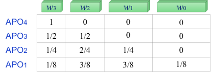
Verification of Property 1 (Early-Mover Advantage): From Eqs. (22)-(25) or from Figure 7 we can easily find that
as by the concavity of .
Verification of Property 2 (Invariance to APO-order Changing): Notice that the MNO’s payoff given in (25) can be rewritten as , which is exactly the expected social welfare when the MNO reaches agreement with each APO with a probability of 0.5. Obviously, changing the order of APOs does not affect the MNO’s payoff.
| Example: Concurrent Bargaining. |
Consider the bargaining between the MNO and an arbitrary APO . The disagreement points (D) of APO and the MNO, and their payoffs (A) and payoff gains (G) if they reach an agreement (and ) are
where and are based on the expectation that the MNO will reach agreements with all other APOs bargaining concurrently. Then, the NBS with APO (i.e., the APO ’s payoff), and the MNO’s payoff under this NBS are
| (26) | ||||
where is the marginal social welfare generated by APO (assuming the MNO will reach agreements with all other APOs).
Verification of Property 3 (Invariance to AP-index Changing): Due to the symmetry of APOs in this example, we have:
That is, the APO’s payoff is independent of its index.
-D Examples of Grouping Effect
Now we use the example in Appendix -C to illustrate the grouping effect. For a better illustration, we consider that APOs and form a new group, denoted by , while APOs and bargain individually. A dummy APO is introduced for the notational consistence. With this APO grouping structure, the bargaining order under the sequential bargaining is , , . By Lemma 2, the traffic offloading profiles are still with this APO grouping structure. Next, we illustrate the payoff profiles under this APO grouping structure.
| Example: Grouping Effect in Sequential Bargaining. |
In Step , the MNO has reached agreements with APO and APO group , and now is bargaining with APO . With a similar analysis in Appendix -C, we can obtain the NBS in Step (i.e., the APO ’s payoff) and the MNO’s payoff under the NBS as follows.
| (27) | ||||
In Step , the MNO has reached agreements with APO , and now is bargaining with the APO group ). The disagreement points (D) of APO group and the MNO, and their payoffs (A) and payoff gains (G) if they reach an agreement (and , ) are
where and are derived from in Step . Note that here is different from that in Appendix -C, as in this new grouping structure, the MNO will not reach an agreement with any APO in under the disagreement outcome. Then, the NBS in Step (i.e., the total payoff of APOs and ), and the MNO’s payoff under this NBS are
| (28) | ||||
where is the virtual marginal social welfare generated by APOs , assuming that the MNO will reach agreement with APO with a probability of 0.5.
In Step , the MNO bargains with the dummy APO ), and thus the bargaining result is straightforward:
| (29) | ||||
In Step , the MNO bargains with APO . with a similar analysis in Appendix -C, we can obtain the NBS in Step (i.e., the APO ’s payoff) and the MNO’s payoff under this NBS as follows.
| (30) | ||||
Verification of Property 5 (Intra-Grouping Benefit): Comparing (28) with (23) and (24), we can find that the total payoff of APOs and increases if they form a group.
Verification of Property 6 (Inter-Grouping Benefit (Positive Externality)): Comparing (30) with (25), we can find that the payoff of APO also increases if APOs and form a group. Furthermore, comparing (27) with (22), the payoff of APO does not change.
| Example: Grouping Effect in Concurrent Bargaining. |
Consider the bargaining between the MNO and an APO (i.e., those not in the group). With a similar analysis in Appendix -C, we can obtain the NBS and the MNO’s payoff under this NBS as follows.
| (31) | ||||
Consider the bargaining between the MNO and the APO group . With a similar analysis, we can obtain the NBS with the APO group and the MNO’s payoff under this NBS as follows.
| (32) | ||||
Verification of Property 7 (Intra-Grouping Benefit): Comparing (32) with (26), we can find that the total payoff of APOs and increases if they form a group (as ).
Verification of Property 8 (No Inter-Group Benefit (Non-Externality)): Comparing (31) with (26), we can find that the payoff of each APO does not change under the new APO grouping structure.
(III) Proofs
-E Proof for Lemma 1 in Section IV
Proof.
To prove this lemma, we only need to prove that the NBS or given in this lemma uniquely solves the problem (9) or (10). Since (10) is a strictly convex optimization problem, it must has a unique solution. Next we solve (10) by sequential optimization on each variable. Specifically, we divide the derivation into two sequential steps: Step-I, finding the optimal under any feasible ; and Step-II, finding the optimal by substituting the optimal into problem (10). The social optimality of the above sequential optimization method is guaranteed by the facts that both sub-problems in the above two steps are convex optimization.
-F Proof for Lemma 2 in Section V-A
Proof: We first show that for any one-to-one bargaining with transferable utility, the disagreement points of bargainers will not affect the achieved social welfare, but only affect the welfare division among bargainers. Then, the bargaining solution must maximize the social welfare, regardless of the disagreement points of bargainers (this result is analytically shown in Section IV.B).
Take the one-to-one bargaining between the MNO and APO as an example. Let and denote the disagreement points of the MNO and the APO , respectively. Then, the NBS between the MNO and APO is given by
| (37) | ||||
where , , and is the NBS between the MNO and other APO . We further notice that
Then, the above optimization problem can be rewritten as
| (38) | ||||
where , and .
It is easy to obtain the following optimal solution for the above problem: (i) , and (ii) is the solution of the following optimization problem
| (39) |
Notice that . We further notice that the terms , , and are independent of . Thus, the above optimization problem is equivalent to the following social welfare maximization problem
| (40) |
That is, the NBS (or in the NBS) between the MNO and APO always maximizes the conditional social welfare, regardless of their disagreement points. Besides, the disagreement points will affect the payment in the NBS, as both and rely on the disagreement points.
Based on the above discussion, we have the following important proposition.
Proposition 1.
Given the NBS between the MNO and every APO , the NBS between the MNO and the APO always maximizes the social welfare , regardless of the disagreement points of the MNO and the APO . That is,
| (41) |
Next we show that under mild conditions, there is a unique bargaining solution for the entire one-to-many bargaining, and such a solution maximizes the overall social welfare.
Notice that the one-to-many bargaining consists of one-to-one bargaining, each corresponding to the bargaining between the MNO and a particular APO. Let denote the NBS between the MNO and every APO , and denote the NBS of the entire one-to-many bargaining, where and . Then, we need to show that the NBS is unique, and solves the social welfare maximization problem
| (42) | ||||
Consider the bargaining between the MNO and a particular APO . By Proposition 1, the NBS (or in the NBS) between the MNO and the APO satisfies:
| (43) |
Thus, the NBS (or in the NBS) of the entire one-to-many bargaining satisfies:
| (44) |
Obviously, the social welfare maximization solution must be a solution of the above equations, since for every . Thus, if there is a unique solution for (44), then it must be .
In general, however, there may have multiple solutions for (44), depending on the form of . To avoid this (multi-solution) situation, we introduce the following assumption:
Assumption 1.
The MNO’s serving cost is an additive function. That is, .
Let denote the MNO’s resource consumption for delivering the traffic within the coverage area of AP , and denote the MNO’s resource consumption for delivering the traffic not within the coverage area of any AP. Obviously, the total resource consumption is . The above assumption implies that
| (45) |
That is, the total serving cost is the summation of the serving costs in all different areas. Notice that in cellular networks, the total serving area is divided into small areas (called cells), and each cell is usually served by a particular base station. Thus, the actual total serving cost of the MNO can be viewed as the summation of the serving costs in all cells. Therefore, the above additive serving cost can be a good approximation to the actual serving cost when the cell size is small enough (hence each cell will not cover many APs), which will become more and more common given the current trend of reducing the cell size to increase the cellular capacity.
Based on this assumption, the MNO’s total serving cost without data offloading is
| (46) |
With data offloading, the MNO’s total serving cost under the offloading profile is
| (47) |
Thus, the serving cost reduction can be written as
| (48) | ||||
where . That is, is also an additive function. Based on the above, we can further rewrite the social welfare as
| (49) | ||||
where . That is, is also an additive function.
Notice that depends only on , while not on , . Thus, we can rewrite the function set (44) as the following equivalent function set.
| (50) |
Obviously, the above function set has a unique solution, since all functions in (50) are decoupled, each having a unique solution (as it is a strictly convex optimization problem).
Denote as the solution of (50). Then,
Thus, we have: for any ,
That is, the solution of (50) maximizes the social welfare.
Based on the above analysis, we can easily obtain the result in Lemma 2. That is, if the MNO’s serving cost is an additive function, then the NBS of the one-to-many bargaining is unique and maximizes the social welfare .
-G Proof for Lemma 3 in Section V-B
Proof.
We first notice that the objective function of (11) is a quadratic function of . Thus, we have the following optimal solution for (11) when there is no constraint in (11):
We next show that the above optimal is located in the feasible set of (11), that is, it satisfies the constraints of (11). Recall that is equivalent to the social welfare maximization solution. Thus, we have:
This implies that , and thus both constraints of (11) are satisfied under the optimal . By independence of irrelevant alternatives (IIA), the above is also the optimal solution of (11) with constraints. ∎
-H Proof for Lemma 4 in Section V-B
Proof.
Similar to Lemma 3, we have the following optimal solution for (14) when there is no constraint in (14):
Thus, we only need to prove that the above optimal satisfies the constraints of (14). Similarly, we first have:
since is the social welfare maximization solution. We further notice that
| (51) |
which implies that the more traffic offloaded to other APs, the less marginal welfare generated by an AP (with the same traffic offloading volume ). By (51), we have:
Based on above, we immediately have:
Thus, both constraints of (14) are satisfied under the optimal given above. ∎
-I Proof for Lemma 5 in Section V-B
Proof.
We prove the lemma by induction. Namely, we can prove the lemma by proving the following two statements:
- •
Statement 1: The NBS in the last Step (for APO ) is characterized by (17);
- •
Proof for Statement 1: By Lemma 3, we can easily find that , which is characterized by (17). Besides, the MNO’s payoff is , which is characterized by (18).
Proof for Statement 2: Suppose that the NBS after Step (i.e., for APOs ) are all characterized by (17). Accordingly, the MNO’s payoff after Step can be characterize by (18). Now we prove that the NBS in Step (i.e., for APO ) is also characterized by (17).
Since the MNO’s payoff in Step can be characterize by (18), we can easily find that when bargaining with APO in Step , the MNO’s disagreement point is
and the MNO’s payoff, if reaching an agreement with APO , is
Thus, the NBS between the MNO and APO is given by the following optimization problem
| (52) | ||||
where .
-J Proof for Theorem 1 in Section V-B
-K Proofs for Properties 1 and 2 in Section V-B
Proof.
We first prove Property 2 (Invariance to AP-order Changing). By (18), the MNO’s payoff can be written as
| (53) | ||||
where . The second line follows because and .
Intuitively, the above MNO’s payoff (53) can be viewed as the average social welfare under such a situation that the MNO and every APO will reach agreement with a probability of 0.5. By (53), we can easily find that the AP-order does not affect the MNO’s payoff in the S-NBS.
We then prove Property 1 (Early-Mover Advantage). Take an arbitrary APO as an example. By Lemma 5, its payoff is
where
Now suppose APO moves backward by one step. That is, APO becomes (denoted by to avoid confusion), and the original APO becomes (denoted by ) in the new bargaining sequence. Then, by Lemma 5, the APO ’s payoff in the new bargaining sequence is
where
The last line follows because and . Here we impliedly use the fact that the social optimal traffic offload profile are identical under any bargaining sequence.
Based on above, we can easily find that
By the concavity of , we further have:
Therefore, we have , that is, APO can achieve a higher payoff when bargaining earlier with the BS.
Intuitively, from (17) we can view the APO ’s payoff as (half of) the average marginal social welfare generated by APO under such a situation that all APOs prior to always reach agreements with the MNO while every posterior APO reaches agreement with the MNO or disagrees with a probability of 0.5. Furthermore, the concavity of implies that the more APOs accept the bargaining solution, the less marginal social welfare generated by an additional APO (under the same traffic offloading volume). Thus, we can immediately find that the APOs bargaining earlier with the MNO is more likely to generate larger average marginal social welfare, and therefore get higher payoff. ∎
-L Proof for Lemma 6 in Section V-B
Proof.
By definition, we can easily find that the NBS between the MNO and the APO is given by
| (54) | ||||
where .
Similar to (11), the objective function of (54) is a quadratic function of . Thus, we have the following optimal solution for (54) when there is no constraint in (54):
Thus, we only need to prove that the above optimal satisfies the constraints of (54). We can easily obtain that
since is the social welfare maximization solution. This implies that , and thus both constraints of (54) are satisfied under the optimal . ∎
-M Proof for Theorem 2 in Section V-B
-N Proofs for Properties 3 and 4 in Section V-B
Proof.
By (19), we can easily prove Properties 3 (Invariance to AP-index Changing). Intuitively, this is because all APOs are symmetric (in terms of the bargaining order) in the concurrent bargaining, and thus the AP-index has no impact on the APO’s payoff.
Compare (19) and (17), we can further find that in the concurrent bargaining, every APO achieves a payoff equal to its payoff in the sequential bargaining when it bargains with the MNO in the last step. By Property 1, this is exactly the worst payoff that it would achieve in the sequential bargaining. ∎
-O Proof for Property 5 in Section V-C
Proof.
For convenience, we focus only on the merge of two successive APOs, say and .1313 13 Note that when studying the merge of two non-successive APs, say and , we have to consider the bargaining order of the merged group and the APO between the APOs in the merged group, i.e., . Later we will show that such a discussion is sufficient, since it leads to the unique outcome where all APOs form a single group.
For notation convenience, we denote the new player (i.e., the merged group ) by . To keep the indexes of APOs , we introduce a dummy APO , that is, APO offers zero resource for data offloading, and receives zero payoff from the MNO. By Lemma 5, the payoff of the new player , i.e., the total payoff of APOs and , is
where
Notice that for dummy AP. Thus, we further have:
Intuitively, is the marginal welfare generated by both APOs and in the group together, suppose the MNO will () or will not () reach an agreement with every posterior APO , . Since is independent of , the total payoff of APOs and (when merging together) can be written as
where
Now we compute the payoffs of APOs , when they bargain independently with the MNO. By Lemma 5, we have
where
Thus, the total payoff of APOs and (when not merging together) can be written as
where
By the concavity of , we can easily find that
This implies that
and therefore . That is, APOs and can achieve a higher total payoff when they merge into a group and bargain with the MNO together. ∎
-P Proof for Property 6 in Section V-C
Proof.
We first study the impact of the merge of APOs and on the payoffs of prior APOs (i.e., those bargaining before APOs and ). Consider an arbitrary APO with . By Lemma 5, its payoff is
where .
Now suppose APOs and merge together. For notation convenience, we denote the merged group by , and introduce a dummy APO to keep the indexes of APOs consistently. Then, the APO ’s payoff under the new group structure is
where
The last line is because and . For convenience, we introduce the following notations:
Then, we can write the APO ’s payoff as follows:
By the concavity of , we further have: . Therefore, we have: , that is, APO can achieve a higher payoff when APOs and merge together.
By similar analysis, we can show that the merge of APOs and and has no impact on the payoff os posterior APOs, i.e., those bargaining after APOs and . ∎
-Q Proof for Property 7 in Section V-C
-R Proof for Property 8 in Section V-C
(IV) An Alternative Modeling Approach
-S Non-cooperative Game Formulation and Analysis
In this section, we formulate the data offload problem as a Stackelberg game based on the non-cooperative game theory, where the MNO acts as the game leader specifying the payments to APOs first, and then every APO acts as a game follower determining the traffic volume it is willing to deliver for the MNO.
We consider a simple linear payment. That is, the payment to an APO is simply defined as a linear function of (i.e., the traffic offload volume to APO ), and denoted by
| (55) |
where is the unit payment to APO for one unit of traffic offload volume. Notice that the transmission efficiency between an APO and its covered MUs is normalized to . Thus, also denotes the amount of APO ’s spectrum resource dedicate to data offload (i.e., to deliver the traffic offloaded from the MNO). In this sense, can also be viewed as the unit price of APO ’s spectrum resource.
With the linear payment, the game process is as follows. In the first stage, the MNO (leader) specifies a price profile , each intending for one APO. In the second stage, every APO responses with , the amount of its resource for data offloading, based on the price and the stochastic distribution of its own traffic demand. An Nash equilibrium (NE) is defined as such a strategy profile such that none of th player can improve its payoff by unilitery deviating. We solve the NE of this game by backward induction.
-S1 The APO’s Decision –
First, we study the APO’s optimal decision in the second stage, given the price specified by the MNO in the first stage. Formally, the decision problem for APO is
| (56) | ||||
where is APO ’s payoff defined in (6).
The first- and second-order derivatives of to are, respectively,
It is easy to see that (since and ). Thus, the problem (56) is a convex optimization, and the optimal solution can be solved using KKT analysis.
Next we present the optimal solution analytically using the FOC analysis. The key idea is that if the FOC condition is achievable, then the optimal is given by the FOC condition in (57). Otherwise, the optimal is the lower-bound or upper-bound of depending on the sign of the first-order derivative.
| (57) |
For convenience, we further introduce the concept of critical price of APO , denoted by
| (58) |
It is important to note that the FOC in (57) is only achievable when . When (or ), however, the first-order derivative is always smaller (or larger) than 0 and never equals to 0, and thus the optimal solution is the lower-bound (or upper-bound) of the feasible range of , i.e., (or ). Formally,
Lemma 7 (APO’s Optimal Decision).
Given the price , every APO ’s optimal decision is
where is the inverse function of .
The first and third cases can be referred to the previous discussion, and the second case is derived from the FOC (57) directly. When the price falls in , we further have
The above formula follows because . Based on above, we have the following properties for .
Property 9.
For any , the optimal satisfies:
- (a)
, that is, increases with ;
- (b)
, if , and vice versa.
The first condition implies that the higher price the MNO offers, the more resource the APO dedicates to data offload. The second condition implies that is an increasing concave (or convex) function of , if has a decreasing (or increasing) PDF . For later derivational convenience, we will assume that , and therefore .1414 14 Note that many common distributions satisfy the condition of decreasing (non-increasing) PDF. Typical examples include uniform distributions, exponential distributions, and power distributions with negative factors, etc.
-S2 The MNO’s Decision –
Now we study the MNO’s best decision in the first stage, based on its prediction of every APO ’s optimal response in the second stage (given in Lemma 7).
Denote as the price profile for all APOs, and as the APOs’ optimal responses. The decision problem for the MNO is
| (59) | ||||
where is the MNO’s payoff defined in (3), and is the pointwise product of vectors and . The element in denotes the payment to every APO.
We first capture some useful information from the first-order partial derivative. Notice that is a function of . The first-order partial derivative of to is
| (60) |
By Lemma 7, we have: , if or . It directly follows that: (i) if , and (ii) if . The first observation implies that any price lower than is indifferent to the MNO, and the second observation implies that any price higher than is dominated by .1515 15 Intuitively, if , APO always returns a zero amount of its resource for data offloading, and thus any price is indifferent to the MNO. If , APO always returns all of its resource for data offloading, and thus a higher price (above ) cannot bring more resource (from APO ) for the MNO, but will definitely lead to a higher payment. Therefore, we can focus on the price below . Formally,
Lemma 8.
For any optimal price profile , the following necessary condition holds:
and in addition, any price below is indifferent.
From (60), we can further find that the optimal price cannot be larger than (since by Lemma 8); otherwise, we will have , which implies that there must exist a price with which the MNO can achieve a higher payoff.1616 16 Here is an arbitrarily small positive number. Therefore, we can focus on the price below . Formally,
Lemma 9.
For any optimal price profile , the following necessary condition holds:
Note that if , then we can directly set as any price lower than , since any price below is indifferent to the MNO.
Then, we study the convexity of the optimization problem (59) by the second-partial partial derivative. Notice that is related to only, while independent of , . The second-order partial derivatives of are
It is easy to see that (i) , since and ; and (ii) , since (by Lemma 9) and (by the assumption of ). Thus, U is concave in . Furthermore, the constraint set of problem (59) is obviously a convex set. Therefore,
Lemma 10.
The problem (59) is a convex optimization.
By the convexity of problem (59), we can solve the problem using classic KKT analysis. Similar to Section V-A, we capture some useful properties of the optimal price profile using the FOC analysis. Suppose all constraints of (59) are strictly satisfied under the optimal solution. Then, the optimal must satisfy the FOC condition:
| (61) |
which leads to the following optimality condition immediately,
Theorem 3 (Optimality).
Suppose all constraints of (59) are not binding. The optimal price profile for the MNO satisfies the following conditions: ,
| (62) |
Now we capture some insight behind the above optimal given in Theorem 3. One one hand, the left hand side of (62) is the marginal cost () of the MNO. On the other hand, the right hand side of (62) is the marginal payment () to APO , i.e., the increase of the MNO’s payment induced by offloading additional units of traffic to APO . Specifically, to increase the traffic offload volume by , the MNO has to increase the price by , which will introduce an additional payment for the existing units of offloaded traffic volume, and a new payment for the coming units of offloaded traffic volume. The equation (62) suggests that in an optimal solution , the equals to the to every APO . Intuitively, if the is larger (or smaller) than the to APO , then the MNO can immediately improve its payoff by offloading more (or less) traffic to APO through increasing (or decreasing) .
By (62), we further have the following property.
Property 10.
Suppose all constraints of (42) are not binding. The optimal price profile satisfies:
| (63) |
where , .
Property 10 states that under the optimal , the MPs to all APOs would be the same. Intuitively, if the , then the MNO can immediately increase its payoff by increasing the traffic volume offloaded to APO and decreasing the traffic volume offloaded to APO .