Stability conditions on $\text{CY}_{N}$ categories associated to $A_{n}$-quivers and period maps

Let $N\geq 2$ be an integer. Here we review the geometric background for this paper and explain why we consider the periods of the differential form $p_{n}(z)^{\frac{N-2}{2}}dz$. Section 2 in [Tho06] is an excellent survey of related topics.

The category $\mathcal{D}_{n}^{N}$ was first introduced as the derived Fukaya category [KS02, Tho06] of Lagrangian $N$-spheres which form the basis of vanishing cycles in the universal deformation of the $A_{n}$-singularity

where $p_{n}(z)=z^{n+1}+u_{1}z^{n-1}+\cdots+u_{n}\,(u_{i}\in\mathbb{C})$ with simple zeros. We consider a symplectic structure on $X^{N}_{p}$ coming from the standard Kähler form on $\mathbb{C}^{N}\times\mathbb{C}$, and a nowhere vanishing holomorphic $N$-form $\Omega_{p}$ on $X^{N}_{p}$ given by taking Poincaré residue of the standard form $dx_{1}\cdots dx_{N}dz$ on $\mathbb{C}^{N+1}$.

Consider the projection

If $z\in\mathbb{C}$ is not a root of $p_{n}$, then the fiber $\pi^{-1}(z)$ is an affine quadric of complex dimension $N-1$ with a real slice $S^{N-1}\subset\pi^{-1}(z)$. Thus, each Lagrangian $N$-sphere is constructed by the total space of the $S^{N-1}$-fibration over a path $\gamma\colon[0,1]\to\mathbb{C}$ which connects distinct roots of $p_{n}$ (see [TY02, Section 6] or [Tho06, Section 2]).

As in [Dou02], a central charge “in the physics literature” of a Lagrangian $L\subset X^{N}_{p}$ is given by the period

Assume that $L$ is a $S^{N-1}$-fibration over the path $\gamma\colon[0,1]\to\mathbb{C}$. Then, up to constant multiplication, the above integration is reduced to the integration of the differential form $p_{n}(z)^{\frac{N-2}{2}}dz$ along the path $\gamma$ (see [TY02, Section 6]):

From this observation, we expect that the central charges of Bridgeland stability conditions on $\mathcal{D}_{n}^{N}$ can be constructed by using the period of the differential form $p_{n}(z)^{\frac{N-2}{2}}dz$.

First we explain the space of polynomials and the associated period map (Section 2). Let $M_{n}$ be the space of polynomials $p_{n}(z)=z^{n+1}+u_{1}z^{n-1}+\cdots+u_{n}\,(u_{i}\in\mathbb{C})$ with $n+1$ simple zeros. Note that the fundamental group of $M_{n}$ is the Artin group $B_{n+1}$. The action of $\mathbb{C}^{*}$ on $M_{n}$ is given by $(u_{1},\dots,u_{n})\mapsto(ku_{1},\dots,k^{n}u_{n})$ for $k\in\mathbb{C}^{*}$.

We regard $p_{n}(z)$ as a meromorphic function on the Riemann sphere $\mathbb{P}^{1}=\mathbb{C}\cup\{\infty\}$. For $p_{n}(z)\in M_{n}$, we define the quadratic differential on $\mathbb{P}^{1}$ by $\phi(z):=p_{n}(z)^{N-2}dz^{\otimes 2}$ and denote by $Q(N,n)$ the space of such differentials.

To consider the period of $\sqrt{\phi}=p_{n}(z)^{\frac{N-2}{2}}dz$, we need to introduce homology groups $H_{+}(\phi)$ and $H_{-}(\phi)$ which provide appropriate cycles for the integration of $\sqrt{\phi}$. If $N$ is even, the homology group is defined by the relative homology group $H_{+}(\phi)=H_{1}(\mathbb{C},\mathrm{Zero}(\phi);\mathbb{Z})$ where $\mathrm{Zero}(\phi)\subset\mathbb{C}$ is the set of zeros of $\phi$. If $N$ is odd, the homology group is defined by $H_{-}(\phi):=H_{1}(S\backslash\pi^{-1}(\infty);\mathbb{Z})$ where $\pi\colon S\to\mathbb{P}^{1}$ is the double cover of the hyperelliptic curve $S=\{y^{2}=p_{n}(z)\}$.

A linear map $Z_{\phi}\colon H_{\pm}(\phi)\longrightarrow\mathbb{C}$, called the period of $\phi$, is defined by

for $\gamma\in H_{\pm}(\phi)$.

Let $\Gamma$ be a free abelian group of rank $n$. An isomorphism of abelian groups $\theta\colon\Gamma\xrightarrow{\sim}H_{\pm}(\phi)$ is called a $\Gamma$-framing of $\phi\in Q(N,n)$. Denote by $Q(N,n)^{\Gamma}$ the set of framed differentials. For a framed differential $(\phi,\theta)\in Q(N,n)^{\Gamma}$, the composition of $\theta\colon\Gamma\to H_{\pm}(\phi)$ and $Z_{\phi}\colon H_{\pm}(\phi)\to\mathbb{C}$ gives a linear map $Z_{\phi}\circ\theta\colon\Gamma\to\mathbb{C}$. We define the period map by

Fix a point $*=(\phi_{0},\theta_{0})\in Q(N,n)^{\Gamma}$ and let $Q(N,n)^{\Gamma}_{*}\subset Q(N,n)^{\Gamma}$ be the connected component containing $*$. Then the universal cover of $Q(N,n)^{\Gamma}_{*}$ is isomorphic to the universal cover $\widetilde{M_{n}}$ of $M_{n}$. Thus the period map $\mathcal{W}_{N}$ is extended on $\widetilde{M_{n}}$:

Next we consider the category $\mathcal{D}_{n}^{N}$ (Section 4) and stability conditions on it (Section 5). For a quiver $Q$, we can define a dg algebra $\Gamma_{N}Q$, called the Ginzburg $\mathrm{CY}_{N}$ dg algebra [Gin]. Let $\mathcal{D}_{\mathrm{fd}}(\Gamma_{N}Q)$ be the derived category of dg modules over $\Gamma_{N}Q$ with finite total dimension. It was proved by Keller [Kel11] that the category $\mathcal{D}_{\mathrm{fd}}(\Gamma_{N}Q)$ is a $\mathrm{CY}_{N}$ triangulated category. Let $Q=\overrightarrow{A_{n}}$ be the $A_{n}$-quiver and set $\mathcal{D}^{N}_{n}:=\mathcal{D}_{\mathrm{fd}}(\Gamma_{N}\overrightarrow{A_{n}})$. An object $S\in\mathcal{D}^{N}_{n}$ is called $N$-spherical if

There is a full subcategory $\mathcal{H}_{0}$, called the standard heart of $\mathcal{D}_{n}^{N}$, and there are $N$-spherical objects $S_{1},\dots,S_{n}\in\mathcal{H}_{0}$ such that $\mathcal{H}_{0}$ is generated by these $N$-spherical objects.

From such objects, Seidel and Thomas defined autoequivalences $\Phi_{S_{1}},\dots,\Phi_{S_{n}}\in\Aut(\mathcal{D}_{n}^{N})$, called spherical twists [ST01]. They also proved that the subgroup $\Sph(\mathcal{D}_{n}^{N})\subset\Aut(\mathcal{D}_{n}^{N})$ generated by $\Phi_{S_{1}},\dots,\Phi_{S_{n}}$ is isomorphic to the braid group $B_{n+1}$.

A stability condition $\sigma=(Z,\mathcal{H})$ on a triangulated category $\mathcal{D}$ consists of a heart $\mathcal{H}\subset\mathcal{D}$ of a bounded t-structure and a linear map $Z\colon K(\mathcal{H})\to\mathbb{C}$ called the central charge, which satisfy some axioms. In [Bri07], Bridgeland showed that the set of stability conditions $\mathrm{Stab}(\mathcal{D})$ has the structure of a complex manifold, and the projection map

is a local isomorphism. There are two group actions on $\mathrm{Stab}(\mathcal{D})$; one is the action of $\mathbb{C}$ and the other is the action of $\Aut(\mathcal{D})$.

Consider the category $\mathcal{D}^{N}_{n}$. There is a distinguished connected component $\mathrm{Stab}^{\circ}(\mathcal{D}_{n}^{N})\subset\mathrm{Stab}(\mathcal{D}_{n}^{N})$ which contains stability conditions with the standard heart $\mathcal{H}_{0}$. The action of the group $\Sph(\mathcal{D}^{N}_{n})$ preserves the connected component $\mathrm{Stab}^{\circ}(\mathcal{D}_{n}^{N})$. Since $\Sph(\mathcal{D}_{n}^{N})\cong B_{n+1}$, the space $\mathrm{Stab}^{\circ}(\mathcal{D}_{n}^{N})$ has the action of the braid group $B_{n+1}$.

Our main result is the following.

When $N=2$, the result was proved by Thomas [Tho06]. When $N=3$ and $n=2$, the result was proved by Sutherland [Sut]. The result for $N=3$ and arbitrary $n$ follows from the result of Bridgeland-Smith [BS15] with some modifications (see Example 12.1 in [BS15]). After submitting this paper on arXiv, I received a preliminary version of the paper [BQS] from Bridgeland, which also proves the result for the case $n=2$ and $2\leq N\leq\infty$ by using a different method. Their approach is based on [Sut], while my approach is based on [BS15].

The result is compatible with the observation in [Bri06] that if there is a Frobenius structure on the space of stability conditions on a $\mathrm{CY}_{N}$ category, then the central charge corresponds to the twisted period of the Frobenius structure with the twist parameter $\nu=(N-2)/\penalty 2$. The twisted periods are characterized as the horizontal sections of the second structure connection of the Frobenius structure with some parameter $\nu$ (see [Dub04, Section 3]). By K. Saito’s theory of primitive forms [Sai83], there is a Frobenius structure on $M_{n}$ and the map $\mathcal{W}_{N}$ naturally arises as the period map associated to the primitive form. As in [Dub04, Section 5], the map $\mathcal{W}_{N}$ coincides with the twisted period map with the parameter $\nu=(N-2)/\penalty 2$. Therefore, the result supports the Bridgeland’s conjecture in [Bri06].

Many arguments of this paper are parallel to those of [BS15] with appropriate generalizations. We replace $\mathrm{CY}_{3}$ categories with $\mathrm{CY}_{N}$ categories, quivers with $(N-2)$-colored quivers, simple zeros with zeros of order $N-2$ and triangulations with $N$-angulations.

However as in Section 6, there are some points where parallel arguments can not be applied. In the case of $N$-angulations, it is not known what objects correspond to quivers with potential and their mutation in the case of triangulations. Hence we do not have natural dg algebras associated to $N$-angulations of surfaces and the categorical equivalence of Keller-Yang [KY11] is not established yet.

Fortunately, King-Qiu’s result [KQ] on the hearts of $\mathcal{D}_{n}^{N}$ together with the geometric realization of the $(N-2)$-cluster category of type $A_{n}$ by Baur-Marsh [BM08] allows us to apply the framework of [BS15] to our cases.

The key idea of constructing stability conditions on $\mathcal{D}_{n}^{N}$ from quadratic differentials is the fact that saddle-free quadratic differentials determine $N$-angulations of surfaces as follows. The differential $\phi$ determines a foliation on $\mathbb{P}^{1}$ by

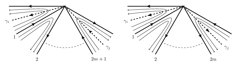
A leaf which connects zeros of $\phi$ is called a saddle trajectory. Near a zero of order $N-2$, the foliation behaves as in Figure 2. As a result, the foliation of a saddle-free differential $\phi$ determines the $N$-angulation $\Delta_{\phi}$ of the $((N-2)(n+1)+2)$-gon (Lemma 6.11) similar to the WKB triangulations in [BS15, GMN]. This is the reason why we consider zeros of order $N-2$. Using the results of Baur-Marsh and King-Qiu, we have a natural heart $\mathcal{H}(\Delta_{\phi})\subset\mathcal{D}_{n}^{N}$ with simple objects $S_{1},\dots,S_{n}$ (Corollary 6.4). Corresponding to these simple objects, there are cycles $\gamma_{1},\dots,\gamma_{n}\in H_{\pm}(\phi)$, called standard saddle classes (Corollary 6.13). The central charge of $S_{i}$ is defined by the period of the corresponding saddle class $\gamma_{i}$:

Thus, we can construct the stability condition $(Z,\mathcal{H}(\Delta_{\phi}))$ on $\mathcal{D}_{n}^{N}$ (Lemma 7.4).

Ishii-Ueda-Uehara [IUU10] proved that the space $\mathrm{Stab}(\mathcal{D}_{n}^{2})$ is connected, so $\mathrm{Stab}^{\circ}(\mathcal{D}_{n}^{2})=\mathrm{Stab}(\mathcal{D}_{n}^{2})$. Together with the result of Thomas in [Tho06], we have $\mathrm{Stab}(\mathcal{D}_{n}^{2})\cong\widetilde{M_{n}}$. In particular, $\mathrm{Stab}(\mathcal{D}_{n}^{2})$ is contractible. For $N\geq 3$, Qiu proved that $\mathrm{Stab}^{\circ}(\mathcal{D}_{n}^{N})$ is simply connected (Corollary 5.5 in [Qiu15]). Our Theorem 1.1 implies the following stronger result (Conjecture 5.8 in [Qiu15]).

The remaining problem is the connectedness of the space $\mathrm{Stab}(\mathcal{D}_{n}^{N})$. As in the case $N=2$, we naively expect the following.

First of all, I am deeply grateful to my advisor Akishi Kato for many valuable discussions, comments, correction of errors and constant encouragement. I would like to thank Kyoji Saito and Atsushi Takahashi for valuable comments on primitive forms. I also would like to thank Fumihiko Sanda for helpful discussions about Fukaya categories.

This work is supported by World Premier International Research Center Initiative (WPI initiative), MEXT, Japan.

This paper is dedicated to the memory of Kentaro Nagao, who explained many basics of this research area and gave me helpful comments at the starting point of this work.

We put $d_{n}^{N}:=(N-2)(n+1)+2$. We work over an algebraically closed field $k$. We use homological gradings $d\colon M_{i}\to M_{i-1}$ for dg algebras and dg modules. Assume that all triangulated categories in this paper are $k$-linear and their Grothendieck groups are free of finite rank ($K(\mathcal{D})\cong\mathbb{Z}^{n}$ for some $n$).

In this section, we introduce the braid groups and their representations on some lattices associated to $A_{n}$-quivers.

It is known that the element

generates the center of $B_{n+1}$.

We consider two representations $\rho_{+}$ and $\rho_{-}$ of $B_{n+1}$ on some lattices associated to the $A_{n}$-quivers. Such representations are equivalent to the reduced Burau representations with the parameters $\pm 1$ (see [KT08, Section 3]).

An $A_{n}$-quiver $\overrightarrow{A_{n}}$ is a quiver obtained by giving orientations on edges of the Dynkin diagram of type $A_{n}$. We set vertices of $\overrightarrow{A_{n}}$ by $\{1,\dots,n\}$ and assume that vertices $i$ and $i+1$ are connected by some arrow. Let $q_{ij}$ be the number of arrows from $i$ to $j$.

Let $L$ be a free abelian group of rank $n$ with generators $\alpha_{1},\dots,\alpha_{n}$:

We define a symmetric bilinear form $\left<\,,\,\right>_{+}$ and a skew-symmetric bilinear form $\left<\,,\,\right>_{-}$ on $L$ by

where $\delta_{ij}$ is the Kronecker delta.

Reflections (which depend on the sign $\pm$) $r_{1}^{\pm},\dots,r_{n}^{\pm}\colon L\to L$ via the bilinear forms $\left<\,,\,\right>_{\pm}$ is defined by

Let $W_{\pm}:=\left<r_{1}^{\pm},\dots,r_{n}^{\pm}\right>$ be the groups generated by these reflections.

Two representations $\rho_{\pm}\colon B_{n+1}\to\GL(L,\mathbb{Z})$ are defined by

We put the kernel of $\rho_{\pm}$ by $P_{\pm}$. Then we have a short exact sequence

Note that the group $W_{+}$ is a symmetric group of degree $n+1$ and the group $P_{+}$ is a pure braid group.

Let $p_{n}(z)$ be a polynomial of the following form

We denote by $\Delta(p_{n})$ the discriminant of $p_{n}$. (If $p_{n}(z)=\prod_{i=1}^{n+1}(z-a_{i})$, then $\Delta(p_{n})=\prod_{i<j}(a_{i}-a_{j})^{2}$.)

Denote by $M_{n}$ the space of such polynomials with simple zeros:

Define the free $\mathbb{C}^{*}$-action on $M_{n}$ by

Note that for the above action, we have the equation

Consider the description of $M_{n}$ as the configuration space of $\mathbb{C}$. Let $C_{n+1}(\mathbb{C})$ be the configuration space of $(n+1)$ distinct points in $\mathbb{C}$ and $C_{n+1}^{0}(\mathbb{C})\subset C_{n+1}(\mathbb{C})$ be the subspace consists of configurations with the center of mass zero:

A complex number $c\in\mathbb{C}$ acts on $C_{n+1}(\mathbb{C})$ as a parallel transportation $(a_{1},\dots,a_{n+1})\mapsto(a_{1}+c,\dots,a_{n+1}+c)$. Hence we have $C_{n+1}^{0}(\mathbb{C})=C_{n+1}(\mathbb{C})/\penalty\mathbb{C}$.

As a result, we have an isomorphism $C_{n+1}^{0}(\mathbb{C})\xrightarrow{\sim}M_{n}$ given by

Next we consider the description of a braid group $B_{n+1}$ as the fundamental group of $M_{n}$. Take a configuration $\{a_{1},\dots,a_{n+1}\}\in C_{n+1}(\mathbb{C})$. We fix some order $(a_{1},\dots,a_{n+1})$ for these $n+1$ points. Consider the collection of non-crossing paths $\gamma_{1},\dots,\gamma_{n}$ in $\mathbb{C}$ such that $\gamma_{i}$ connects $a_{i}$ and $a_{i+1}$. We call it the $A_{n}$-chain of paths. Let $\tau_{i}$ be a closed path in $C_{n+1}(\mathbb{C})$ which corresponds to the half-twist along $\gamma_{i}$ in the clockwise direction (see Figure 1), and consider its image in $M_{n}$ via the projection $C_{n+1}(\mathbb{C})\to M_{n}$ (we also write it by $\tau_{i}$).

It is well-known that there is an isomorphism of groups

For more details, we refer to [KT08, Section 1.6].

Let $\mathbb{P}^{1}$ be the Riemann sphere, and we fix the coordinate $z\in\mathbb{C}\cup\{\infty\}\cong\mathbb{P}^{1}$. For a polynomial $p_{n}\in M_{n}$, define the meromorphic quadratic differential $\phi$ on $\mathbb{P}^{1}$ by

$\phi$ has zeros of order $(N-2)$ at distinct $n+1$ points on $\mathbb{C}\subset\mathbb{P}^{1}$, and a unique pole of order $(d_{n}^{N}+2)$ at $\infty\in\mathbb{P}^{1}$.

We denote by $Q(N,n)$ the space of such quadratic differentials associated to $p_{n}\in M_{n}$:

Independent of $N$, the space $Q(N,n)$ is isomorphic to $M_{n}$ as a complex manifold, but we give this space various structures which depend on $N$.

We introduce the action of $\mathbb{C}^{*}$ on $Q(N,n)$. For $\phi(z)=p_{n}(z)^{N-2}dz^{\otimes 2}$, the action of $\mathbb{C}^{*}$ is defined by

where $k\cdot p_{n}$ is the action defined in Section 2.2. By using the equation $(k\cdot p_{n})(kz)=k^{n+1}p_{n}(z)$, we have the following formula.

For $\phi\in Q(N,n)$, denote by $\mathrm{Zero}(\phi)\subset\mathbb{P}^{1}$ the set of zeros of $\phi$ and by $\mathrm{Crit}(\phi)\subset\mathbb{P}^{1}$ the set of critical points of $\phi$. Note that $\mathrm{Crit}(\phi)=\mathrm{Zero}(\phi)\cup\{\infty\}$.

The action $z\mapsto kz$ of $k\in\mathbb{C}^{*}$ on $\mathbb{P}^{1}$ maps the critical points of $\phi$ to those of $k\cdot\phi$:

Note that if $N=3$, the homology group $H_{-}(\phi)$ corresponds to the hat-homology group in [BS15] which is written as $\hat{H}(\phi)$.

Proof. If $N$ is even, $|\mathrm{Zero}(\phi)|=n+1$ implies $\rank H_{+}(\phi)=n$.

If $N$ is odd, there are two cases, $n$ is even or odd. If $n$ is even, the genus of the hyperelliptic curve $S$ is $n/\penalty 2$ and the fiber $\pi^{-1}(\infty)$ consists of one point. Hence we have $\rank H_{-}(\phi)=2(n/\penalty 2)=n$. When $n$ is odd, the genus of $S$ is $(n-1)/\penalty 2$ and the fiber $\pi^{-1}(\infty)$ consists of two points. Hence we have $\rank H_{-}(\phi)=2\{(n-1)/\penalty 2\}+1=n$. $\square$

Let $\psi:=\sqrt{\phi}=p_{n}(z)^{\frac{N-2}{2}}\,dz$ be the square root of $\phi$. (If $N$ is odd, $\psi$ is determined up to the sign.) If $N$ is even, then $\psi$ is a holomorphic $1$-form on $\mathbb{P}^{1}\,\backslash\,\{\infty\}$, and if $N$ is odd, then $\psi$ is a holomorphic $1$-form on $S\,\backslash\,\pi^{-1}(\infty)$.

Therefore, for any cycle $\alpha\in H_{\pm}(\phi)$ the integration of $1$-form $\psi$ via the cycle $\alpha$

is well-defined.

Thus we have a group homomorphism $Z_{\phi}\colon H_{\pm}(\phi)\to\mathbb{C}$, called the period of $\phi$.

Following [BS15, Section 2.6], we introduce framings on $Q(N,n)$. Let $\Gamma$ be a free abelian group of rank $n$. A $\Gamma$-framing of $\phi\in Q(N,n)$ is an isomorphism of abelian groups

Denote by $Q(N,n)^{\Gamma}$ the space of pairs $(\phi,\theta)$ consisting of a quadratic differential $\phi\in Q(N,n)$ and a $\Gamma$-framing $\theta$. The projection

defines a principal $\GL(n,\mathbb{Z})$-bundle on $Q(N,n)$.

For $(\phi,\theta)\in Q(N,n)^{\Gamma}$, the composition of a framing $\theta$ and a period $Z_{\phi}$ gives a group homomorphism $Z_{\phi}\circ\theta\colon\Gamma\to\mathbb{C}$. Thus, we have the map

defined by $\mathcal{W}_{N}((\phi,\theta)):=Z_{\phi}\circ\theta\in\Hom_{\mathbb{Z}}(\Gamma,\mathbb{C})$. We call $\mathcal{W}_{N}$ a period map.

Proof. Theorem 4.12 in [BS15] can be easily extended to our cases. In our cases, the result also follows from K. Saito’s theory on primitive forms [Sai83, Section5] since $\mathcal{W}_{N}$ is interpreted as the period map associated to the primitive form of the $A_{n}$-singularity. $\square$

In this section, we introduce intersection forms on $H_{\pm}(\phi)$.

First we consider the case $N$ is even. The exact sequence of relative homology groups gives the isomorphism of homology groups

where $\widetilde{H}_{0}(\mathrm{Zero}(\phi);\mathbb{Z})$ is the reduced homology group of $H_{0}(\mathrm{Zero}(\phi);\mathbb{Z})$, and this isomorphism is induced by the boundary map. There is a trivial intersection form on $H_{0}(\mathrm{Zero}(\phi);\mathbb{Z})$, and it induces the intersection form on $\widetilde{H}_{0}(\mathrm{Zero}(\phi);\mathbb{Z})$. Through the above isomorphism of homology groups, we have the intersection form

Note that $I_{+}$ is symmetric and non-degenerate.

Next consider the case $N$ is odd. Let $\pi\colon S\to\mathbb{P}^{1}$ be the hyperelliptic curve introduced in Section 2.4, and $\iota\colon S\,\backslash\,\pi^{-1}(\infty)\to S$ be the inclusion. This inclusion induces the surjective group homomorphism

Since there is a skew-symmetric non-degenerate intersection form on $H_{1}(S;\mathbb{Z})$, through the inclusion $\iota_{*}$, we have the intersection form

The map $\iota_{*}$ is an isomorphism if $n$ is even and has the kernel of rank one if $n$ is odd. Therefore, $I_{-}$ is non-degenerate if $n$ is even or has the kernel of rank one if $n$ is odd.

For $\phi\in Q(N,n)$, fix the order of $\mathrm{Zero}(\phi)$ and consider the $A_{n}$-chain of path $\gamma_{1},\dots,\gamma_{n}$. If $N$ is even, the path $\gamma_{i}$ determines the homology class $\hat{\gamma}_{i}\in H_{+}(\phi)$ since $\gamma_{i}$ connects zeros of $\phi$. If $N$ is odd, since the lift $\pi^{-1}(\gamma_{i})$ on the hyperelliptic curve $S$ is a closed path in $S\backslash\pi^{-1}(\infty)$, we have the homology class $\hat{\gamma}_{i}:=[\pi^{-1}(\gamma_{i})]\in H_{-}(\phi)$.

The pair of the homology group $H_{\pm}(\phi)$ and the intersection form $I_{\pm}$ gives a geometric realization of the lattice $(L,\left<\,,\,\right>_{\pm})$ which is introduced in Section 2.1.

Proof. The result follows from the direct calculation. $\square$

For each $\phi\in Q(N,n)$, by corresponding to the homology group $H_{\pm}(\phi)$, we have a local system

For a continuous path $c\colon[0,1]\to Q(N,n)$ with $\phi_{0}=c(0),\,\phi_{1}=c(1)$, a parallel transportation along $c$ gives the identification

and this identification determines a flat connection on the local system. We call it the Gauss-Manin connection.

In the following, we fix a point $(\phi_{0},\theta_{0})\in Q(N,n)^{\Gamma}$ and denote by $Q(N,n)^{\Gamma}_{*}$ the connected component containing $(\phi_{0},\theta_{0})$. Any point $(\phi,\theta)\in Q(N,n)^{\Gamma}$ is contained in $Q(N,n)^{\Gamma}_{*}$ if and only if there is a continuous path $c\colon[0,1]\to Q(N,n)$ connecting $\phi_{0}$ and $\phi$ such that the diagram

commutes.

Note that different connected components of $Q(N,n)^{\Gamma}$ are all isomorphic since these are related by the action of $\GL(n,\mathbb{Z})$.

We introduce the $\mathbb{C}$-action on $Q(N,n)^{\Gamma}_{*}$, which is compatible with the $\mathbb{C}$-action on the space of stability conditions given in Section 5.3.

By using the intersection form $I_{\pm}$ on $H_{\pm}(\phi)$ defined in Section 2.6, we can compute how cycles change by the Gauss-Manin connection along a closed path in $Q(N,n)$. The result is known as the Picard-Lefschetz formula.

Let $\phi_{0}=\left[\prod_{i=1}^{n+1}(z-a_{i})\right]^{N-2}dz^{\otimes 2}$ be the fixed differential in the previous section. Take the $A_{n}$-chain of paths $\gamma_{1},\dots,\gamma_{n}$ for ordered zeros $(a_{1},a_{2},\dots,a_{n+1})$ as in Section 2.2. Under the identification $M_{n}\cong Q(N,n)$, we consider the half-twists $\tau_{1},\dots,\tau_{n}$ as in Section 2.2 and take the orientations of $\hat{\gamma}_{1},\dots,\hat{\gamma}_{n}\in H_{\pm}(\phi_{0})$ as in Lemma 2.6.

References

• [Ami09] C Amiot. Cluster categories for algebras of global dimension 2 and quivers with potential. Ann. Inst. Fourier (Grenoble), 59(6):2525–2590, 2009.
• [BBD82] A. A. Beĭlinson, J. Bernstein, and P. Deligne. Faisceaux pervers. In Analysis and topology on singular spaces, I (Luminy, 1981), volume 100 of Astérisque, pages 5–171. Soc. Math. France, Paris, 1982.
• [BM08] K. Baur and R. J. Marsh. A geometric description of mm-cluster categories. Trans. Amer. Math. Soc., 360(11):5789–5803, 2008.
• [Bri06] T. Bridgeland. Stability conditions on a non-compact Calabi-Yau threefold. Comm. Math. Phys., 266(3):715–733, 2006.
• [Bri07] T. Bridgeland. Stability conditions on triangulated categories. Ann. of Math., 166(2):317–345, 2007.
• [Bri09] T. Bridgeland. Spaces of stability conditions. In Algebraic geometry—Seattle 2005. Part 1, volume 80 of Proc. Sympos. Pure Math., pages 1–21. Amer. Math. Soc., Providence, RI, 2009.
• [BS15] T. Bridgeland and I. Smith. Quadratic differentials as stability conditions. Publ. Math. de l’IHES., 121:155–278, 2015.
• [BQS] T. Bridgeland, Y. Qiu and T. Sutherland. Stability conditions and the A2A_{2} quiver. arXiv:1406.2566.
• [BT09] A. B. Buan and H. Thomas. Coloured quiver mutation for higher cluster categories. Adv. Math., 222(3):971–995, 2009.
• [Dou02] R. Douglas. Dirichlet branes, homological mirror symmetry, and stability. In Proceedings of the International Congress of Mathematicians, Vol. III (Beijing, 2002), pages 395–408, Beijing, 2002. Higher Ed. Press.
• [Dub04] B. Dubrovin. On almost duality for Frobenius manifolds. In Geometry, topology, and mathematical physics, volume 212 of Amer. Math. Soc. Transl. Ser. 2., pages 75–132. Amer. Math. Soc, Providence, RI, 2004.
• [Gin] V. G. Ginzburg. Calabi-Yau algebras. arXiv:math/0612139.
• [GMN] D. Gaiotto, G. Moore, and A. Neitzke. Wall-crossing, Hitchin Systems, and the WKB Approximation. arXiv:0907.3987.
• [HRS96] D. Happel, I. Reiten, and S. O. Smalø. Tilting in abelian categories and quasitilted algebras. Mem. Amer. Math. Soc., 120(575):viii+ 88, 1996.
• [IUU10] A. Ishii, K. Ueda, and H. Uehara. Stability conditions on AnA_{n}-singularities. J. Differential Geom., 84(1):87–126, 2010.
• [Kel11] B Keller. Deformed Calabi-Yau completions. J. Reine Angew. Math., 654:125–180, 2011. With an appendix by Michel Van den Bergh.
• [KN13] B. Keller and P. Nicolás. Weight structures and simple dg modules for positive dg algebras Int. Math. Res. Not., 1028–1078, 2013.
• [KQ] K. King and Y. Qiu. Exchange graphs and Ext quivers. to appear in Adv. Math., arXiv:1109.2924v3.
• [KS] M. Kontsevich and Y. Soibelman. Stability structures, motivic Donaldson-Thomas invariants and cluster transformations. arXiv:0811.2435.
• [KS02] M. Khovanov and P. Seidel. Quivers, floer cohomology, and braid group actions. J. Amer. Math. Soc., 15:203–271, 2002.
• [KT08] C. Kassel and V. Turaev. Braid groups, volume 247 of Graduate Texts in Mathematics. Springer, New York, 2008. With the graphical assistance of Olivier Dodane.
• [KY11] B. Keller and D. Yang. Derived equivalences from mutations of quivers with potential. Adv. Math., 226(3):2118–2168, 2011.
• [Qiu15] Y. Qiu. Stability conditions and quantum dilogarithm identities for Dynkin quivers. Adv. Math., 269:220–264, 2015.
• [Sai83] K. Saito. Period Mapping Associated to a Primitive Form. In Publ. RIMS. 19:1231–1264, 1983.
• [ST01] P. Seidel and R. P. Thomas. Braid group actions on derived categories of coherent sheaves. Duke Math. J., 108(1):37–108, 2001.
• [Str84] K Strebel. Quadratic differentials, volume 5 of Ergebnisse der Mathematik und ihrer Grenzgebiete (3) [Results in Mathematics and Related Areas (3)]. Springer-Verlag, Berlin, 1984.
• [Sut] T. Sutherland. The modular curve as the space of stability conditions of a CY3 algebra. arXiv:1111.4184.
• [Tho06] R. P. Thomas. Stability conditions and the braid group. Comm. Anal. Geom., 14(1):135–161, 2006.
• [TY02] R.P. Thomas and S.T. Yau. Special Lagrangians, stable bundles and mean curvature flow. Comm. Anal. Geom., 10:1075–1113, 2002.
• [Woo10] J. Woolf. Stability conditions, torsion theories and tilting. J. Lon. Math. Soc., 82:663–682, 2010.