Fundamental Limits of Caching in Wireless D2D NetworksThanks: The authors are with the Department of Electrical Engineering, University of Southern California, Los Angeles, CA 90089, USA. (e-mail: {mingyuej, caire, molisch}@usc.edu)

Motivated by the above question, in this paper we consider the same model of D2D wireless networks as in [5, 8], with a caching and delivery scheme inspired by [10], based on subpacketization in the caching phase and (inter-session) coding in the delivery phase. Our main contributions are as follows: 1) if each node in the network can reach in a single hop all other nodes in the network, the proposed scheme achieves almost the same throughput of [10], without the need of a central base station; 2) if the transmission range of each node is limited, such that concurrent short range transmissions can co-exist in a spatial reuse scheme, then the throughput has the same scaling law (with possibly different leading term constants) of the reuse-only case [5, 8] or the coded-only case [10]. This result holds even if one optimizes the transmission range and therefore the spatial reuse of the system. Counterintuitively, this means that it is not possible to cumulate the spatial reuse gain and the coded multicasting gain, and that these two albeit different type of gains are equivalent as far as the throughput scaling law is concerned. Beyond scaling laws, in order to establish the best combination of reuse and coded multicasting gains, trading off the rate achieved on each local link (decreasing function of distance) with the number of users that can be reached by a coded multicast message (increasing function of distance), must be sought in terms of the actual throughput in bit/s/Hz (i.e., in the coefficients of the dominant terms of the throughput scaling for large $n,m$ and finite $M$, and not just in the scaling law itself).

We consider both deterministic caching and (decentralized) random caching (as done in [21] for the single bottleneck link case). In both cases, we show that for most regimes of the system parameters (apart from the regime of very small caches, which is not really relevant for applications), the throughput achieved with both the proposed deterministic and random caching schemes is optimal within a constant factor.

The paper is organized as follows. Section II presents the network model and the formal problem definition. We illustrate all the main results based on the deterministic caching scheme and its implications in Section III. In Section IV, we discuss the decentralized caching scheme and the corresponding coded delivery approach. Section V contains our concluding remarks and the main proofs are given in Appendices in order to keep the flow of exposition.

Before proceeding in the presentation of our results, we would like to make a few remarks to clarify obvious questions and anticipate possible concerns that this line of work (see for example [10, 21, 22, 23, 3, 2, 7, 24, 25, 26, 5, 8, 6, 27, 28, 29, 30, 31, 32]) may raise.

First, we would like to point out that in this paper we refer to “coding” in the sense of “inter-session network coding”, i.e., when the codeword is a function of symbols (or, “subpackets”) from different source messages (files in the library). Often, coding at the application layer [33, 34, 35] or right on top of the transport layer [36] is used in an intra-session only mode, in order to send linear combinations of subpackets from the same source message and cope with packet losses in the network, but without mixing subpackets of different messages. We point out that this intra-session “packet erasure coding” has conceptually little to do with “network coding”, although it has been sometimes referred to as “random linear network coding” when the linear combinations are generated with randomly drawn coefficients over some finite field. In line with [10] and with the protocol model of our previous work [5, 8], also in this paper any transmission within the appropriate range is assumed to be “noiseless” (i.e., perfectly decoded) and therefore we will not consider packet erasure coding against channel impairments.

Then, it is important to notice that this work, as well as [5, 8, 10], is based on an underlying time-scale decomposition for which the caching phase (i.e., placing information in the caches) is done “a priori”, at some time scale much slower than the delivery phase (i.e., satisfying the users demands). For example, we may imagine that the caches content is updated every day, through a conventional cellular network used during off-peak time, such that the content library is refreshed by inserting new titles and deleting old ones. This scenario differs significantly with respect to the conventional and widely studied “on-line” caching policies, where the cache content is updated along with the delivery process [37, 38, 39, 40, 41, 42, 43].

Finally, we would like to mention here that the considerations made in [5, 10, 21] about handling asynchronous demands holds verbatim in this paper, and shall not be repeated for the sake of brevity. It should be clear that although we consider (for simplicity of exposition) files of the same length, the schemes described in this paper generalize immediately (with the same fundamental performance) to the case of unequal length files and asynchronous demands.

The following theorem yields the achievable rate of the proposed caching and coded multicasting delivery scheme.

The caching and delivery scheme achieving (6) is given in Appendix A and an illustrative example is given in Section III-C. The proof of Theorem 1 is given in Appendix B. The corresponding achievable throughput is given by the following immediate corollary:

In this case, the transmission range can be chosen in order to have localized D2D communication and therefore allow for some spatial reuse. In this case, we need to design also a transmission policy to schedule concurrent active links. The proposed policy is based on clustering: the network is divided into clusters of equal size $g_{c}$, independently of the users’ demands. Users can receive messages only from nodes in the same cluster. Therefore, each cluster is treated as a small network. Assuming that $g_{c}M\geq m$,⁶⁶ 6 If the condition $g_{c}M\geq m$ is not satisfied, we can choose a larger transmission range such that this condition is feasible. the total cache capacity of each cluster is sufficient to store the whole file library. Under this assumption, the same caching and delivery scheme used to prove Theorem 1 can be used here. A simple achievable transmission policy consists of partitioning the set of clusters into ${\cal K}$ reuse sets, such that the clusters of the same reuse set do not interfere and can be active simultaneously. In each active cluster, a single transmitter is active per time-slot and it is received by all the nodes in the cluster, as in classical time-frequency reuse schemes with reuse factor ${\cal K}$ currently used in cellular networks [44, Ch. 17]. An example of a reuse set is shown in Fig. 1. In particular, we can pick ${\cal K}=\left(\left\lceil\sqrt{2}(1+\Delta)\right\rceil+1\right)^{2}$. This scheme achieves the following throughput:

The proof of Theorem 4 is given in Appendix E. Notice that whether reuse is convenient or not in this context depends on whether $C_{\sqrt{2}}$ (the link spectral efficiency for communicating across the network) is larger or smaller than $C_{r}/{\cal K}$, for some smaller $r$ which determines the cluster size. In turns, this depends on the how the link spectral efficiency varies as a function of the communication range. This aspect is not captured by the protocol model, and the answer may depend on the operating frequency and appropriate channel model of the underlying wireless network physical layer [6].

An upper bound on the throughput with reuse is given by:

The proof of Theorem 5 is given in Appendix F. Furthermore, we have:

The proof of Theorem 6 is given in Appendix G. Similar to the case of $r\geq\sqrt{2}$, when $L=L^{\prime}$ (i.e., when naive multicasting is possible), we can show that $\frac{T^{*}(M)}{T(M)}$ is upper bounded by the constant factor, independent of $m$, $n$ and $M$.

The proposed caching placement and delivery scheme and the techniques of the proof for the converse are illustrated through a simple example. Consider a network with three users ($n=3$). Each user can store $M=2$ files, and the library has size $m=3$ files, which are denoted by $A,B,C$. Let $r\geq\sqrt{2}$. Without loss of generality, we assume that each node requests one packet of a file ($L^{\prime}=1$). We divide each packet of each file into $6$ subpackets, and denote the subpackets of the $j$-th packet as $\{A_{j,\ell}:\ell=1,\ldots,6\}$, $\{B_{j,\ell}:\ell=1,\ldots,6\}$, and $\{C_{j,\ell}:\ell=1,\ldots,6\}$. The size of each subpacket is $F/6$. We let user $u$ stores $Z_{u}$, $u=1,2,3$, given as follows:

In this example, we consider the demand ${\sf f}=(A,B,C)$. Since the request vector contains distinct files, specifying which segment of each file is requested (i.e., the vector ${\sf s}$) is irrelevant and shall be omitted. In the coded delivery phase (see Fig. 2), user $1$ multicasts $B_{3}+C_{1}$ (useful to both user 2 and 3), user $2$ multicasts $A_{5}+C_{2}$ (useful to both users 1 and 3) and user $3$ multicasts $A_{6}+B_{4}$ (useful to both users 1 and 2). It follows that $R(2)=R_{1}+R_{2}+R_{3}=\frac{1}{6}\cdot 3=\frac{1}{2}$ is achievable.

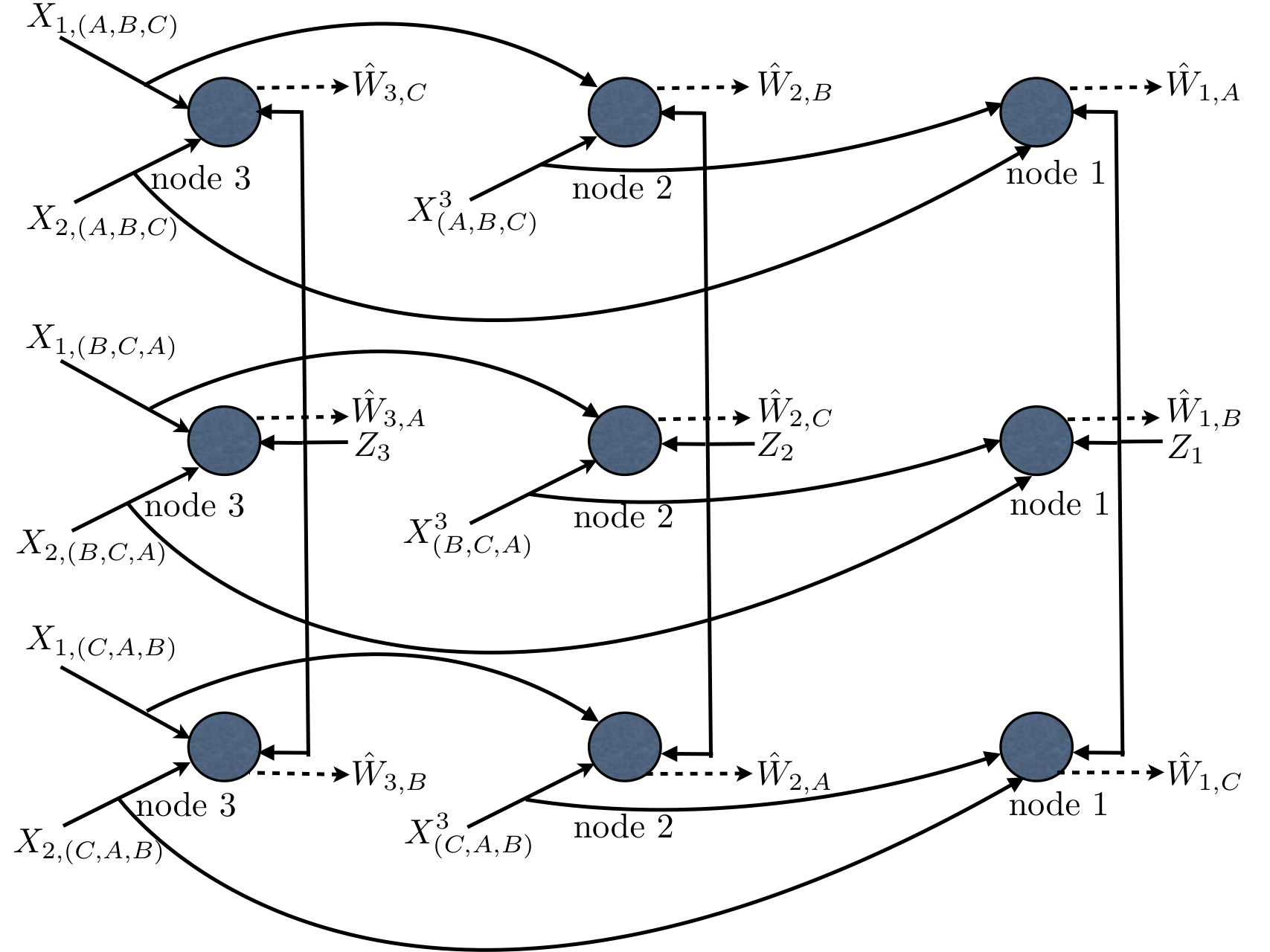
Next, we illustrate the idea of the general rate lower bound of Theorem 2. Without loss of generality, we assume that $L/L^{\prime}$ is an integer and let $s$ denote the segment index. For any scheme that satisfies arbitrary demands ${\sf f}$, with arbitrary segments ${\sf s}$, we denote by $R_{u,s,{\sf f}}^{\rm T}$ the number of coded bits transmitted by user $u$, relative to segment $s$ and request vector ${\sf f}$. Since the requests are arbitrary, we can consider a compound extension for all possible request vectors. For example, we let the first request be ${\sf f}=(A,B,C)$, the second request be ${\sf f}=(B,C,A)$ and the third request be ${\sf f}=(C,A,B)$. Then, the augmented compound-extended graph is shown in Fig. 3 where, consistently with our general notation defined in Section II, $Z_{u}$ denotes the cached symbols at user $u=1,2,3$, $X_{u,{\sf f}}$ denotes the transmitted message from user $u$ in correspondence of demand ${\sf f}$, and $\hat{W}_{u,f}$ is the decoded message at user $u$ relative to file $f$. Considering user 3, from the cut that separates $(X_{1,(A,B,C)},X_{2,(A,B,C)},X_{1,(B,C,A)},X_{2,(B,C,A)},X_{1,(C,A,B)},X_{2,(C,A,B)},Z_{3})$ and $(\hat{W}_{3,C},\hat{W}_{3,A},\hat{W}_{3,B})$, and by using the fact that the sum of the entropies of the received messages and the entropy of the side information (cache symbols) cannot be smaller than the number of requested information bits, we obtain that

Similarly, from the cut that separates $(X_{1,(A,B,C)}$, $X_{3,(A,B,C)}$, $X_{1,(B,C,A)}$, $X_{3,(B,C,A)}$, $X_{1,(C,A,B)}$, $X_{3,(C,A,B)}$, $Z_{2})$ and $(\hat{W}_{2,B},\hat{W}_{2,C},\hat{W}_{2,A})$, and from the cut that separates $(X_{2,(A,B,C)}$, $X_{3,(A,B,C)}$, $X_{2,(B,C,A)}$, $X_{3,(B,C,A)}$, $X_{2,(C,A,B)}$, $X_{3,(C,A,B)}$, $Z_{1})$ and $(\hat{W}_{1,A},\hat{W}_{1,B},\hat{W}_{1,C})$, we obtain analogous inequalities up to index permutations. By summing (18) and the other two corresponding inequalities and dividing all terms by 2, we obtain

Since we are interested in minimizing the worst-case rate, the sum $R^{T}_{1,s,{\sf f}}+R^{T}_{2,s,{\sf f}}+R^{T}_{3,s,{\sf f}}$ must yields the same min-max value $R^{\rm T}$ for any ${\sf s}$ and ${\sf f}$. This yields the bound

Finally, by definition of rate $R(M)$, we have that $R(M)=R^{T}/(FL^{\prime})$. Therefore, dividing both sides of (19) by $3FL$, we obtain that the best possible achievable rate must satisfy

In the example of this section, for $M=2$ we obtain $R^{*}(2)\geq\frac{1}{2}$. Therefore, in this case the achievability scheme given before is information theoretically optimal.

In the same case of $n=3$ users, per-node storage capacity $M=2$ and library size $m=3$, the coded multicasting scheme of [10] where a single codeword is sent to all users through a common bottleneck link achieves $R(2)=\frac{1}{3}$. Then, in this case, the relative loss incurred by not having a base station with access to all files is $3/2$.

The achievable rate of Theorem 1 can be written as the product of three terms, $R(M)=n\left(1-\frac{M}{m}\right)\frac{m}{Mn}$ with the following interpretation: $n$ is the number of transmissions by using a conventional scheme that serves individual demands without exploiting the asynchronous content reuse; $\left(1-\frac{M}{m}\right)$ can be viewed as the local caching gain, since any user can cache a fraction $M/m$ of any file, therefore it needs to receive only the remaining part; $\frac{m}{Mn}$ is the global caching gain, due to the ability of the scheme to turn the individual demands into a coded multicast message, such that transmissions are useful to many users despite the streaming sessions are strongly asynchronous. An analogous interpretation can be given for the terms appearing in the rate expression achievable with the scheme presented in [10] (see Section I), where the base station has access to all the files. Comparing this rate with our Theorem 1, we notice that they differ only in the last term (global caching gain), which in the base station case is given by $(1+\frac{nM}{m})^{-1}$. For $nM\gg m$, we notice that these factors are essentially identical.

As already noticed, Theorem 4 shows that there is no fundamental cumulative gain by using both spatial reuse and coded multicasting. Under our assumptions, spatial reuse may or may not be convenient, depending whether $\frac{C_{r}}{{\cal K}}$ is larger or smaller than $C_{\sqrt{2}}$. A closer look reveals a more subtle tradeoff. Without any spatial reuse, let $t=\frac{Mn}{m}\in\mathbb{Z}^{+}$, the length of the codewords in coded subpackets for each user, related to the size of the subpacketization, is $t{n\choose t}$. This may be very large when $n$ and $M$ are large. At the other extreme, we have the case where the cluster size is the minimum able to cache the whole library in each cluster. In this case, we can just store $M$ different whole files into each node, such that all $m$ files are present in each cluster, and for the delivery phase we just serve whole files without any coding as in [5]. In this case, the achieved throughput is $\frac{C_{r}}{{\cal K}}\frac{M}{m}$ bits/s/Hz, which is almost as good as the coded scheme, which achieves $\frac{C_{r}}{{\cal K}\left(\frac{m}{M}-1\right)}$. This simple scheme is a special case of the general setting treated in this paper, where spatial reuse is maximized and codewords have length 1. If we wish to use the achievable scheme of this paper, the codewords length is $\frac{Mg_{c}}{m}{g_{c}\choose\frac{Mg_{c}}{m}}$. Hence, spatial reuse yields a reduction in the codeword length of the corresponding coded multicasting scheme.

Further, we also notice that even though our scheme is design for a D2D system, it can also be used in a peer-to-peer (P2P) wired network, where each peer is allowed to cache information with limited storage capacity. By using our approach in the case of $r\geq\sqrt{2}$, peers can exchange multicast messages which are useful for a large number of other peers, provided that the network supports multicasting.

Decentralized random caching with coded multicast delivery has been considered in [21]. However, there is an important difference between our network model and that of [21], where, thanks to the central omniscient server (base station), possibly missing packets due to the decentralized random caching can always be supplied by the server by unicasting (or naive multicasting). In our system this is not possible, since no node has generally access to the whole file library. Hence, in order to ensure a vanishing probability of error, we shall use an additional layer of Maximum Distance Separable (MDS) coding and consider the limit of large packet size $F$.

We distinguish between two regimes: $t\stackrel{{\scriptstyle\Delta}}{{=}}\frac{Mn}{m}>1$ and $t=1$. As already noticed before, $t<1$ is not valid since in this case the file library cannot be cached into the network and therefore the worst case user demands cannot be satisfied.

For $t>1$, we consider the following scheme: each file segment of $F$ bits is divided into $K$ blocks of $F/K$ bits each, hereafter referred to as “subpackets”. These subpackets are interpreted as the elements of the binary extension field $\mbox{\bb F}_{2^{F/K}}$, and are encoded using a $(K,K/\rho)$-MDS code, for some $\rho<1$ the choice of which will be discussed later. Notice that this expands the size of each packet from $F$ to $F/\rho$. The resulting $K/\rho$ encoded blocks of $F/K$ bits each will be referred to as “MDS-coded symbols”. The definition of worst-case error probability and achievable rates given in Section II hold verbatim in this case. In particular, since the definition of achievable rate considers a sequence of coding schemes for $F\rightarrow\infty$, we can choose $K$ as a function of $F$ such that both $K$ and $F/K$ grow unbounded as $F$ increases. This ensures that, for any fixed $\rho$, $(K,K/\rho)$-MDS codes exist [45, 46]. The MDS-coded symbols are cached at random by the user nodes according to Algorithm 1.

Next, we describe a delivery scheme that provides to each requesting user enough MDS-coded symbols such that it can recover the desired file segments. For $k=1,\cdots,L^{\prime}$, let $s_{u}+k-1$ denote the index of the $k$-th requested packet of file $f_{u}$ by user $u$. Let $\{Z_{f}^{i,j}:j=1,\cdots,K/\rho\}$ denote the block of MDS-coded symbols from packet $i$ of file $f$. For $b=n,n-1,\ldots,2$, and each user subset ${\sf U}\subseteq\mathcal{U}$ of size $|{\sf U}|=b$, we define $Z_{f_{u},{\sf U}\backslash\{u\}}^{s_{u}+k-1}$ as the symbol sequence obtained by concatenating (in any pre-determined order) the symbols needed by $u\in{\sf U}$, present in all the caches of users $v\in{\sf U}\backslash\{u\}$, and not present in the cache of any other user $v^{\prime}\notin{\sf U}\backslash\{u\}$. We refer to $Z_{f_{u},{\sf U}\backslash\{u\}}^{s_{u}+k-1}$ as the symbols relative ot $u\in{\sf U}$ and exclusively cached in all nodes $v\in{\sf U}\backslash\{u\}$. Formally, the index set of the symbols forming $Z_{f_{u},{\sf U}\backslash\{u\}}^{s_{u}+k-1}$ is given by

where the index set does not depend on the packet index $s_{u}+k-1$ since the same caching rule is used for all packets (see Algorithm 1). Then, $Z_{f_{u},{\sf U}\backslash\{u\}}^{s_{u}+k-1}$ is the sequence of MDS-coded symbols formed by concatenating the symbols $\{Z_{f_{u}}^{s_{u}+k-1,j}:j\in J_{f_{u},{\sf U}\backslash\{u\}}\}$. By construction, each user $v\in{\sf U}$ has one local replica of $Z_{f_{u},{\sf U}\backslash\{u\}}^{s_{u}+k-1}$ (common symbols) for each $u\in{\sf U}\backslash\{v\}$. We also let $J_{{\sf U}}^{\rm max}=\max_{u\in{\sf U}}|J_{f_{u},{\sf U}\backslash\{u\}}|$, such that all sequences $Z_{f_{u},{\sf U}\backslash\{u\}}^{s_{u}+k-1}$ can be zero-padded⁷⁷ 7 With a slight abuse of notation we indicate by $Z_{f_{u},{\sf U}\backslash\{u\}}^{s_{u}+k-1}$ also the zero-padded version. to the common maximum length $J_{{\sf U}}^{\rm max}$. In order to deliver the MDS-coded symbols, each user $v\in{\sf U}\backslash\{u\}$ sends distinct (i.e., non-overlapping) segments of length $\frac{1}{b-1}\cdot J_{{\sf U}}^{\rm max}\cdot\frac{F}{K}$ of the sequence of XORed MDS-coded symbols $\bigoplus_{u\in{\sf U},u\neq v}Z_{f_{u},{\sf U}\backslash\{u\}}^{s_{u}+k-1}$. The delivery phase is summarized in Algorithm 2.

Since the scheme is admittedly complicated and its general description relies on a heavy notation, we provide here an illustrative example (see Fig. 4). As in the case of deterministic caching, consider the case of 3 users denoted by 1,2,3. Neglecting the packet superscript (irrelevant in this example), for the first round of the scheme, with $b=3$ (see Fig. 4), let $Z_{f_{1},\{2,3\}}$ be the sequence of MDS-coded symbols useful to user 1 (requesting file $f_{1}$) and present in the caches of users 2 and 3. Also, let $Z_{f_{2},\{1,3\}}$ and $Z_{f_{3},\{1,2\}}$ have similar and corresponding meaning, after permuting the indices. Then, user 1 forms the XORed sequence $Z_{f_{2},\{1,3\}}\oplus Z_{f_{3},\{1,2\}}$, user 2 forms the XORed sequence $Z_{f_{1},\{2,3\}}\oplus Z_{f_{3},\{1,2\}}$, and user 3 forms the XORed sequence $Z_{f_{1},\{2,3\}}\oplus Z_{f_{2},\{1,3\}}$. Finally, each user transmits to the other two users $1/2$ of its own XORed sequence. For the second round of the scheme, with $b=2$ (see Fig. 4), let $Z_{f_{1},\{2\}}$ and $Z_{f_{1},\{3\}}$ denote the sequence of MDS-coded symbols useful to user 1 and cached exclusively by user 2 and user 3, respectively. Similarly, let $Z_{f_{2},\{1\}}$, $Z_{f_{2},\{3\}}$, $Z_{f_{3},\{1\}}$ and $Z_{f_{3},\{2\}}$ have corresponding meaning. Since $b=2$, there is no multicasting opportunity. User 1 will just transmit sequence $Z_{f_{2},\{1\}}$ to user 2 and $Z_{f_{3},\{1\}}$ to user 3. Users 2 and 3 perform similar operations. Focusing on decoding at user 1, after the first round, half of $Z_{f_{1},\{2,3\}}$ is recovered from user 2 transmission and the other half from user 3 transmission, by using the side information of its own cache. After the second round, $Z_{f_{1},\{2\}}$ is directly received from user 2, and $Z_{f_{1},\{3\}}$ from user 3. Finally, if the MDS coding rate $\rho$ is chosen appropriately, user 1 is able to recover the desired file $f_{1}$ with high probability from the MDS-coded symbols $Z_{f_{1},\{2,3\}},Z_{f_{1},\{2\}}$ and $Z_{f_{1},\{3\}}$ and the symbols relative to file $f_{1}$ already present in its cache.

The following result yields a sufficient condition for the MDS coding rate $\rho$ such that, in the general case, all files can be decoded with high probability from the MDS coded symbols cached in the network:

Theorem 7 is proved in Appendix H. From Theorem 7 and the union bound, we have immediately that all the files can be successfully decoded from the cached MDS-coded symbols in the network with arbitrarily high probability for sufficiently large $K$.

References

- [1] “http://www.cisco.com/en/US/solutions/collateral/ns341/ns525/ns537 /ns705/ns827/white/paper/c11-520862.html.,” .
- [2] N. Golrezaei, A.F. Molisch, A.G. Dimakis, and G. Caire, “Femtocaching and device-to-device collaboration: A new architecture for wireless video distribution,” Communications Magazine, IEEE, vol. 51, no. 4, pp. 142–149, 2013.
- [3] N. Golrezaei, K. Shanmugam, A. G. Dimakis, A. F. Molisch, and G. Caire, “Femtocaching: Wireless video content delivery through distributed caching helpers,” in INFOCOM, 2012 Proceedings IEEE. IEEE, 2012, pp. 1107–1115.
- [4] N. Golrezaei, M. Ji, A. F. Molisch, A. G. Dimakis, and G. Caire, “Device-to-device communications for wireless video delivery,” in Signals, Systems and Computers (ASILOMAR), 2012 Conference Record of the Forty Sixth Asilomar Conference on. IEEE, 2012, pp. 930–933.
- [5] M. Ji, G. Caire, and A. F. Molisch, “Optimal throughput-outage trade-off in wireless one-hop caching networks,” in Information Theory Proceedings (ISIT), 2013 IEEE International Symposium on. IEEE, 2013, pp. 1461–1465.
- [6] M. Ji, G. Caire, and A. F Molisch, “Wireless device-to-device caching networks: Basic principles and system performance,” arXiv preprint arXiv:1305.5216, 2013.
- [7] S. Gitzenis, G.S. Paschos, and L. Tassiulas, “Asymptotic laws for joint content replication and delivery in wireless networks,” IEEE Trans. on Inform. Theory, vol. 59, no. 5, pp. 2760–2776, May 2013.
- [8] M. Ji, G. Caire, and A.F. Molisch, “The throughput-outage tradeoff of wireless one-hop caching networks,” arXiv preprint arXiv:1302.2168, 2013.
- [9] P. Gupta and P.R. Kumar, “The capacity of wireless networks,” Information Theory, IEEE Transactions on, vol. 46, no. 2, pp. 388–404, 2000.
- [10] M.A. Maddah-Ali and U. Niesen, “Fundamental limits of caching,” arXiv preprint arXiv:1209.5807, 2012.
- [11] Z. Bar-Yossef, Y. Birk, T.S. Jayram, and T. Kol, “Index coding with side information,” Information Theory, IEEE Transactions on, vol. 57, no. 3, pp. 1479–1494, 2011.
- [12] S. El Rouayheb, A. Sprintson, and C. Georghiades, “On the index coding problem and its relation to network coding and matroid theory,” Information Theory, IEEE Transactions on, vol. 56, no. 7, pp. 3187–3195, 2010.
- [13] E. Lubetzky and U. Stav, “Nonlinear index coding outperforming the linear optimum,” Information Theory, IEEE Transactions on, vol. 55, no. 8, pp. 3544–3551, 2009.
- [14] A. Blasiak, R. Kleinberg, and E. Lubetzky, “Index coding via linear programming,” arXiv preprint arXiv:1004.1379, 2010.
- [15] M. Chaudhry, Z. Asad, A. Sprintson, and M. Langberg, “On the complementary index coding problem,” in Information Theory Proceedings (ISIT), 2011 IEEE International Symposium on. IEEE, 2011, pp. 244–248.
- [16] S. Jafar, “Topological interference management through index coding,” 2013.
- [17] Ishay Haviv and Michael Langberg, “On linear index coding for random graphs,” in Information Theory Proceedings (ISIT), 2012 IEEE International Symposium on. IEEE, 2012, pp. 2231–2235.
- [18] F. Arbabjolfaei, B. Bandemer, Y.H. Kim, E. Sasoglu, and L. Wang, “On the capacity region for index coding,” in Information Theory Proceedings (ISIT), 2013 IEEE International Symposium on. IEEE, 2013, pp. 962–966.
- [19] S. Unal and A.B. Wagner, “General index coding with side information: Three decoder case,” in Information Theory Proceedings (ISIT), 2013 IEEE International Symposium on, July 2013, pp. 1137–1141.
- [20] E. Nygren, R. K. Sitaraman, and J. Sun, “The akamai network: a platform for high-performance internet applications,” ACM SIGOPS Operating Systems Review, vol. 44, no. 3, pp. 2–19, 2010.
- [21] M. A. Maddah-Ali and U. Niesen, “Decentralized caching attains order-optimal memory-rate tradeoff,” arXiv preprint arXiv:1301.5848, 2013.
- [22] R. Pedarsani, M.A. Maddah-Ali, and U. Niesen, “Online coded caching,” arXiv preprint arXiv:1311.3646, 2013.
- [23] U. Niesen and M. Maddah-Ali, “Coded caching with nonuniform demands,” arXiv preprint arXiv:1308.0178, 2013.
- [24] J Llorca, A.M. Tulino, K Guan, J Esteban, M Varvello, N Choi, and D Kilper, “Dynamic in-network caching for energy efficient content delivery,” in INFOCOM, 2013 Proceedings IEEE. IEEE, 2013, pp. 245–249.
- [25] J Llorca, A.M. Tulino, K Guan, J Esteban, M Varvello, N Choi, and D Kilper, “Network-coded caching-aided multicast for efficient content delivery,” in ICC, 2013 Proceedings IEEE. IEEE, 2013.
- [26] J Llorca and A.M. Tulino, “The content distribution problem and its complexity classification,” Alcatel-Lucent technical report, 2013.
- [27] M. Ji, G. Caire, and A.F. Molisch, “Fundamental limits of distributed caching in d2d wireless networks,” in Information Theory Workshop (ITW), 2013 IEEE. IEEE, 2013, pp. 1–5.
- [28] M. Ji, A.M. Tulino, J. Llorca, and G. Caire, “Order optimal coded caching-aided multicast under zipf demand distributions,” arXiv preprint arXiv:1402.4576, 2014.
- [29] M. Ji, A.M. Tulino, J. Llorca, and G. Caire, “Order optimal coded delivery and caching: Multiple groupcast index coding,” arXiv preprint arXiv:1402.4572, 2014.
- [30] A. Sengupta, R. Tandon, and T.C. Clancy, “Fundamental limits of caching with secure delivery,” arXiv preprint arXiv:1312.3961, 2013.
- [31] N Karamchandani, Maddah-Ali.M.A. Niesen, N, and S. Diggavi, “Hierarchical coded caching: divide and conquer,” in ITA. IEEE, 2014.
- [32] J. Hachem, N. Karamchandani, and S. Diggavi, “On wireless content distribution,” in ITA. IEEE, 2014.
- [33] A. Shokrollahi, “Raptor codes,” Information Theory, IEEE Transactions on, vol. 52, no. 6, pp. 2551–2567, 2006.
- [34] M. Luby, M. Watson, T. Gasiba, T. Stockhammer, and W. Xu, “Raptor codes for reliable download delivery in wireless broadcast systems,” in Consumer Communications and Networking Conference, 2006. CCNC 2006. 3rd IEEE. IEEE, 2006, vol. 1, pp. 192–197.
- [35] S. Aditya and S. Katti, “Flexcast: graceful wireless video streaming,” in Proceedings of the 17th annual international conference on Mobile computing and networking. ACM, 2011, pp. 277–288.
- [36] J. K. Sundararajan, D. Shah, Muriel Médard, Michael Mitzenmacher, and Joao Barros, “Network coding meets tcp,” in INFOCOM 2009, IEEE. IEEE, 2009, pp. 280–288.
- [37] A. Meyerson, K. Munagala, and S. Plotkin, “Web caching using access statistics,” in Proceedings of the twelfth annual ACM-SIAM symposium on Discrete algorithms. Society for Industrial and Applied Mathematics, 2001, pp. 354–363.
- [38] L. W. Dowdy and D. V. Foster, “Comparative models of the file assignment problem,” ACM Computing Surveys (CSUR), vol. 14, no. 2, pp. 287–313, 1982.
- [39] A. Dan, D. Sitaram, and P. Shahabuddin, “Dynamic batching policies for an on-demand video server,” Multimedia systems, vol. 4, no. 3, pp. 112–121, 1996.
- [40] M. R. Korupolu, C. G. Plaxton, and R. Rajaraman, “Placement algorithms for hierarchical cooperative caching,” in Proceedings of the tenth annual ACM-SIAM symposium on Discrete algorithms. Society for Industrial and Applied Mathematics, 1999, pp. 586–595.
- [41] I. Baev, R. Rajaraman, and C. Swamy, “Approximation algorithms for data placement problems,” SIAM Journal on Computing, vol. 38, no. 4, pp. 1411–1429, 2008.
- [42] S. Borst, V. Gupta, and A. Walid, “Distributed caching algorithms for content distribution networks,” in INFOCOM, 2010 Proceedings IEEE. IEEE, 2010, pp. 1–9.
- [43] K. C. Almeroth and M. H. Ammar, “The use of multicast delivery to provide a scalable and interactive video-on-demand service,” Selected Areas in Communications, IEEE Journal on, vol. 14, no. 6, pp. 1110–1122, 1996.
- [44] A.F. Molisch, Wireless communications, 2nd edition, IEEE Press - Wiley, 2011.
- [45] S. Lin and D. J. Costello, Error control coding, vol. 123, Prentice-hall Englewood Cliffs, 2004.
- [46] R. W. Yeung, Information theory and network coding, Springer, 2008.
- [47] T. Ho, M. Médard, R. Koetter, D. R Karger, M. Effros, J. Shi, and B. Leong, “A random linear network coding approach to multicast,” Information Theory, IEEE Transactions on, vol. 52, no. 10, pp. 4413–4430, 2006.
- [48] Y. Sánchez de la Fuente, T. Schierl, C. Hellge, T. Wiegand, D. Hong, D. De Vleeschauwer, W. Van Leekwijck, and Y. Le Louédec, “idash: improved dynamic adaptive streaming over http using scalable video coding,” in Proceedings of the second annual ACM conference on Multimedia systems. ACM, 2011, pp. 257–264.
- [49] L. Keller, A. Le, B. Cici, H. Seferoglu, C. Fragouli, and A. Markopoulou, “Microcast: Cooperative video streaming on smartphones,” in ACM MobiSys. ACM, 2012, pp. 57–70.
- [50] X. Wu, S. Tavildar, S. Shakkottai, T. Richardson, J. Li, R. Laroia, and A. Jovicic, “Flashlinq: A synchronous distributed scheduler for peer-to-peer ad hoc networks,” in Communication, Control, and Computing (Allerton), 2010 48th Annual Allerton Conference on. IEEE, 2010, pp. 514–521.
- [51] D. Camps-Mur, A. Garcia-Saavedra, and P. Serrano, “Device to device communications with wifi direct: overview and experimentation,” IEEE Wireless Communications Magazine, 2012.
- [52] K. Doppler, M. Rinne, C. Wijting, C. B. Ribeiro, and K. Hugl, “Device-to-device communication as an underlay to lte-advanced networks,” Communications Magazine, IEEE, vol. 47, no. 12, pp. 42–49, 2009.
- [53] T. Rappaport, F. Gutierrez, E. Ben-Dor, J. Murdock, Y. Qiao, and J. Tamir, “Broadband millimeter wave propagation measurements and models using adaptive beam antennas for outdoor urban cellular communications,” 2011.
- [54] Y. Azar, G. N. Wong, K. Wang, R. Mayzus, Jocelyn K. S., H. Zhao, F. Gutierrez, D. Hwang, and T. S. Rappaport, “28 ghz propagation measurements for outdoor cellular communications using steerable beam antennas in new york city,” in 2013 IEEE International Conference on Communications (2013 ICC), 2013.
- [55] R. C. Daniels, J. N. Murdock, T. S. Rappaport, and R. W. Heath, “60 ghz wireless: Up close and personal,” Microwave Magazine, IEEE, vol. 11, no. 7, pp. 44–50, 2010.
- [56] M. R. Akdeniz, Y. Liu, S. Sun, S. Rangan, T. S. Rappaport, and E. Erkip, “Millimeter wave channel modeling and cellular capacity evaluation,” arXiv preprint arXiv:1312.4921, 2013.
- [57] S. Rangan, T. Rappaport, E. Erkip, Z. Latinovic, M. R. Akdeniz, and Y. Liu, “Energy efficient methods for millimeter wave picocellular systems,” Communications, 2013.
- [58] S. Rangan, T. S. Rappaport, and E. Erkip, “Millimeter wave cellular wireless networks: Potentials and challenges,” arXiv preprint arXiv:1401.2560, 2014.
- [59] S. Boucheron, G. Lugosi, and P. Massart, Concentration Inequalities: A Nonasymptotic Theory of Independence, Oxford University Press, 2013.