跳到论文正文
W Papers独立论文阅读器 arXiv:1405.5195 论文正文 计算阅读时间 · 0%
引用这篇论文根据当前论文元数据生成,正式投稿前建议核对。


License: arXiv.org perpetual non-exclusive license
arXiv:1405.5195v2 [cs.IT] 17 Dec 2015

Capacity of a Class of State-Dependent Orthogonal Relay ChannelsThanks:  This paper was presented in part at the IEEE Information Theory Workshop (ITW), Laussane, Switzerland, Sept. 2012 [1]. I. Estella Aguerri is with the Mathematical and Algorithmic Sciences Laboratory, France Research Center, Huawei Technologies Company, Ltd., Boulogne-Billancourt 92100, France E-mail: inaki.estella@huawei.com. Deniz Gündüz is with the Department of Electrical and Electronic Engineer, Imperial College London, London SW7 2BT, U.K. E-mail: d.gunduz@imperial.ac.uk. The research presented here was done during the Ph.D. studies of Iñaki Estella Aguerri at Imperial College London.

Iñaki Estella Aguerri and Deniz Gündüz Affiliation: 
Abstract

The class of orthogonal relay channels in which the orthogonal channels connecting the source terminal to the relay and the destination, and the relay to the destination, depend on a state sequence, is considered. It is assumed that the state sequence is fully known at the destination while it is not known at the source or the relay. The capacity of this class of relay channels is characterized, and shown to be achieved by the partial decode-compress-and-forward (pDCF) scheme. Then the capacity of certain binary and Gaussian state-dependent orthogonal relay channels are studied in detail, and it is shown that the compress-and-forward (CF) and partial-decode-and-forward (pDF) schemes are suboptimal in general. To the best of our knowledge, this is the first single relay channel model for which the capacity is achieved by pDCF, while pDF and CF schemes are both suboptimal. Furthermore, it is shown that the capacity of the considered class of state-dependent orthogonal relay channels is in general below the cut-set bound. The conditions under which pDF or CF suffices to meet the cut-set bound, and hence, achieve the capacity, are also derived.

Index Terms: 
Capacity, channels with state, relay channel, decode-and-forward, compress-and-forward, partial decode-compress-and forward.

I Introduction

We consider a state-dependent orthogonal relay channel, in which the channels connecting the source to the relay, and the source and the relay to the destination are orthogonal, and are governed by a state sequence, which is assumed to be known only at the destination. We call this model the state-dependent orthogonal relay channel with state information available at the destination, and refer to it as the ORC-D model. See Figure 1 for an illustration of the ORC-D channel model.

Many practical communication scenarios can be modelled by the ORC-D model. For example, consider a cognitive network with a relay, in which the transmit signal of the secondary user interferes simultaneously with the received primary user signals at both the relay and the destination. After decoding the secondary user’s message, the destination obtains information about the interference affecting the source-relay channel, which can be exploited to decode the primary transmitter’s message. Note that the relay may be oblivious to the presence of the secondary user, and hence, may not have access to the side information. Similarly, consider a mobile network with a relay (e.g., a femtostation), in which the base station (BS) operates in the full-duplex mode, and transmits on the downlink channel to a user, in parallel to the uplink transmission of a femtocell user, causing interference for the uplink transmission at the femtostation. While the femtostation, i.e., the relay, has no prior information about this interfering signal, the BS knows it perfectly and can exploit this knowledge to decode the uplink user’s message forwarded by the femtostation.

The best known transmission strategies for the three terminal relay channel are the decode-and-forward (DF), compress-and-forward (CF) and partial decode-compress-and-forward (pDCF) schemes, which were all introduced by Cover and El Gamal in [2]. In DF, the relay decodes the source message and forwards it to the destination together with the source terminal. DF is generalized by the partial decode-and-forward (pDF) scheme in which the relay decodes and forwards only a part of the message. In the ORC-D model, pDF would be optimal when the channel state information is not available at the destination [3]; however, when the state information is known at the destination, fully decoding and re-encoding the message transmitted on the source-relay link renders the channel state information at the destination useless. Hence, we expect that pDF is suboptimal for ORC-D in general.

In CF, the relay does not decode any part of the message, and simply compresses the received signal and forwards the compressed bits to the destination using Wyner-Ziv coding followed by separate channel coding. Using CF in the ORC-D model allows the destination to exploit its knowledge of the state sequence; and hence, it can decode messages that may not be decodable by the relay. However, CF also forwards some noise to the destination, and therefore, may be suboptimal in certain scenarios. For example, as the dependence of the source-relay channel on the state sequence weakens, i.e., when the state information becomes less informative, CF performance is expected to degrade.

pDCF combines both schemes: part of the source message is decoded by the relay, and forwarded, while the remaining signal is compressed and forwarded to the destination. Hence, pDCF can optimally adapt its transmission to the dependence of the orthogonal channels on the state sequence. Indeed, we show that pDCF achieves the capacity in the ORC-D channel model, while pure DF and CF are in general suboptimal. The main results of the paper are summarized as follows:

  • •

    We derive an upper bound on the capacity of the ORC-D model, and show that it is achievable by the pDCF scheme. This characterizes the capacity of this class of relay channels.

  • •

    Focusing on the multi-hop binary and Gaussian models, we show that applying either only the CF or only the DF scheme is in general suboptimal.

  • •

    We show that the capacity of the ORC-D model is in general below the cut-set bound. We identify the conditions under which pure DF or pure CF meet the cut-set bound. Under these conditions the cut-set bounds is tight, and either DF or CF scheme is sufficient to achieve the capacity.

While the capacity of the general relay channel is still an open problem, there have been significant achievements within the last decade in understanding the capabilities of various transmission schemes, and the capacity of some classes of relay channels has been characterized. For example, DF is shown to be optimal for physically degraded relay channels and inversely degraded relay channels in [2]. In [3], the capacity of the orthogonal relay channel is characterized, and shown to be achieved by the pDF scheme. It is shown in [4] that pDF achieves the capacity of semi-deterministic relay channels as well. CF is shown to achieve the capacity in deterministic primitive relay channels in [5]. While all of these capacity results are obtained by using the cut-set bound for the converse proof [6], the capacity of a class of modulo-sum relay channels is characterized in [7], and it is shown that the capacity, achievable by the CF scheme, can be below the cut-set bound. The pDCF scheme is shown to achieve the capacity of a class of diamond relay channels in [8].

The state-dependent relay channel has also attracted considerable attention in the literature. Key to the investigation of the state-dependent relay channel model is whether the state sequence controlling the channel is known at the nodes of the network, the source, relay or the destination in a causal or non-causal manner. The relay channel in which the state information is non-causally available only at the source is considered in [9, 10], and both causally and non-causally available state information is considered in [11]. The model in which the state is non-causally known only at the relay is studied in [12] while causal and non-causal knowledge is considered in [13]. Similarly, the relay channel with state causally known at the source and relay is considered in [14], and state non-causally known at the source, relay and destination in [15]. Recently a generalization of pDF, called the cooperative-bin-forward scheme, has been shown to achieve the capacity of state-dependent semi-deterministic relay channels with causal state information at the source and destination [16]. The compound relay channel with informed relay and destination are discussed in [17] and [18]. The state-dependent relay channel with structured state has been considered in [19] and [20]. To the best of our knowledge, this is the first work that focuses on the state-dependent relay channel in which the state information is available only at the destination.

The rest of the paper is organized as follows. In Section II we provide the system model and our main result. Section III is devoted to the proofs of the achievability and converse for the main result. In Section IV, we provide two examples demonstrating the suboptimality of pDF and CF schemes on their own, and in Section V we show that the capacity is in general below the cut-set bound, and we provide conditions under which pure DF and CF schemes meet the cut-set bound. Finally, Section VII concludes the paper.

We use the following notation in the rest of the paper: Xij≜(Xi,Xi+1,…,Xj)X_{i}^{j}\triangleq(X_{i},X_{i+1},...,X_{j}) for i<ji<j, Xn≜(X1,…,Xn)X^{n}\triangleq(X_{1},...,X_{n}) for the complete sequence, Xn+1n≜∅X_{n+1}^{n}\triangleq\emptyset, and Zn∖i≜(Z1,…,Zi−1,Zi+1,…,Zn)Z^{n\setminus i}\triangleq(Z_{1},...,Z_{i-1},Z_{i+1},...,Z_{n}).

II System Model and Main Result

We consider the class of orthogonal relay channels depicted in Figure 1. The source and the relay are connected through a memoryless channel characterized by p⁡(yR|x1,z)p(y_{R}|x_{1},z), the source and the destination are connected through an orthogonal memoryless channel characterized by p⁡(y2|x2,z)p(y_{2}|x_{2},z), while the relay and the destination are connected by a memoryless channel p⁡(y1|xR,z)p(y_{1}|x_{R},z). The three memoryless channels depend on an independent and identically distributed (i.i.d.) state sequence {Z}i=1n\{Z\}_{i=1}^{n}, which is available at the destination. The input and output alphabets are denoted by 𝒳1\mathcal{X}_{1}, 𝒳2\mathcal{X}_{2}, 𝒳R\mathcal{X}_{R}, 𝒴1\mathcal{Y}_{1}, 𝒴2\mathcal{Y}_{2} and 𝒴R\mathcal{Y}_{R}, and the state alphabet is denoted by 𝒵\mathcal{Z}.

Refer to caption
Fig. 1: Orthogonal state-dependent relay channel with channel state information available at the destination, called the ORC-D model.

Let WW be the message to be transmitted to the destination with the assistance of the relay. The message WW is assumed to be uniformly distributed over the set 𝒲={1,…,M}\mathcal{W}=\{1,...,M\}. An (M,n,νn)(M,n,\nu_{n}) code for this channel consists of an encoding function at the source:

f:{1,…,M}→𝒳1n×𝒳2n,\displaystyle f:\{1,...,M\}\rightarrow\mathcal{X}_{1}^{n}\times\mathcal{X}_{2}^{n}, (1)

a set of encoding functions {fr,i}i=1n\{f_{r,i}\}_{i=1}^{n} at the relay, whose output at time ii depends on the symbols it has received up to time i−1i-1:

XR​i=fr,i(YR​1,…,YR⁡(i−1)),i=1,…,n,\displaystyle X_{Ri}=f_{r,i}(Y_{R1},...,Y_{R(i-1)}),\quad i=1,...,n, (2)

and a decoding function at the destination

g:𝒴1n×𝒴2n×𝒵n→{1,…,M}.\displaystyle g:\mathcal{Y}_{1}^{n}\times\mathcal{Y}_{2}^{n}\times\mathcal{Z}^{n}\rightarrow\{1,...,M\}. (3)

The probability of error, νn\nu_{n}, is defined as

νn≜1M​∑w=1MPr​{g⁡(Y1n,Y2n,Zn)≠w|W=w}.\displaystyle\nu_{n}\triangleq\frac{1}{M}\sum_{w=1}^{M}\text{Pr}\{g(Y_{1}^{n},Y_{2}^{n},Z^{n})\neq w|W=w\}. (4)

The joint probability mass function (pmf) of the involved random variables over the set 𝒲×𝒵n×𝒳1n×𝒳2n×𝒳Rn×𝒴Rn×𝒴1n×𝒴2n\mathcal{W}\times\mathcal{Z}^{n}\times\mathcal{X}_{1}^{n}\times\mathcal{X}_{2}^{n}\times\mathcal{X}_{R}^{n}\times\mathcal{Y}_{R}^{n}\times\mathcal{Y}_{1}^{n}\times\mathcal{Y}_{2}^{n} is given by

p(w,zn,x1n,x2n,xRn,yRn,y1n,y2n)=p(w)∏i=1np(zi)p(x1​i,x2​i|w)⋅\displaystyle p(w,z^{n},x_{1}^{n},x_{2}^{n},x_{R}^{n},y_{R}^{n},y_{1}^{n},y_{2}^{n})\!=\!p(w)\prod_{i=1}^{n}p(z_{i})p(x_{1i},x_{2i}|w)\cdot
p⁡(yR​i|zi,x1​i)​p​(xR​i|yRi−1)​p​(y1​i|xR​i,zi)​p​(y2​i|x2​i,zi).\displaystyle p(y_{Ri}|z_{i},x_{1i})p(x_{Ri}|y_{R}^{i-1})p(y_{1i}|x_{Ri},z_{i})p(y_{2i}|x_{2i},z_{i}).

A rate RR is said to be achievable if there exists a sequence of (2n​R,n,νn)(2^{nR},n,\nu_{n}) codes such that limn→∞νn=0\lim_{n\rightarrow\infty}\nu_{n}=0. The capacity, 𝒞\mathcal{C}, of this class of state-dependent orthogonal relay channels, denoted as ORC-D, is defined as the supremum of the set of all achievable rates.

We define R1R_{1} and R1R_{1} as follows, which can be thought as the capacities of the individual links from the relay to the destination, and from the source to the destination, respectively, when the channel state sequence is available at the destination:

R1≜maxp⁡(xR)⁡I⁡(XR;Y1|Z),R2≜maxp⁡(x2)⁡I⁡(X2;Y2|Z).\displaystyle R_{1}\triangleq\max_{p(x_{R})}I(X_{R};Y_{1}|Z),\quad R_{2}\triangleq\max_{p(x_{2})}I(X_{2};Y_{2}|Z). (5)

Let p∗​(xR)p^{*}(x_{R}) and p∗​(x2)p^{*}(x_{2}) be the channel input distributions achieving R1R_{1} and R2R_{2}, respectively.

Let us define 𝒫\mathcal{P} as the set of all joint pmf’s given by

𝒫≜{p(u,x1,z,yR,y^R):\displaystyle\mathcal{P}\triangleq\{p(u,x_{1},z,y_{R},\hat{y}_{R}): (6)
p(u,x1,z,yR,y^R)=p(u,x1)p(z)p(yR|x1,z)p(y^R|yR,u)},\displaystyle p(u,x_{1},z,y_{R},\hat{y}_{R})=p(u,x_{1})p(z)p(y_{R}|x_{1},z)p(\hat{y}_{R}|y_{R},u)\},

where UU and Y^R\hat{Y}_{R} are auxiliary random variables defined over the alphabets 𝒰\mathcal{U} and 𝒴^R\mathcal{\hat{Y}}_{R}, respectively.

The main result of this work, provided in the next theorem, is the capacity of the class of relay channels described above.

Theorem 1.

The capacity of the ORC-D relay channel is given by

𝒞=\displaystyle\mathcal{C}= sup𝒫\displaystyle\sup_{\mathcal{P}}\, R2+I⁡(U,YR)+I⁡(X1;Y^R|U​Z),\displaystyle R_{2}+I(U;Y_{R})+I(X_{1};\hat{Y}_{R}|UZ), (7)
s.t. R1≥I⁡(U,YR)+I⁡(YR;Y^R|U​Z),\displaystyle R_{1}\geq I(U;Y_{R})+I(Y_{R};\hat{Y}_{R}|UZ),

where |𝒰|≤|𝒳1|+3|\mathcal{U}|\leq|\mathcal{X}_{1}|+3 and |𝒴^R|≤|𝒰|​|𝒴R|+1|\mathcal{\hat{Y}}_{R}|\leq|\mathcal{U}||\mathcal{Y}_{R}|+1.

Proof.

The achievability part of the theorem is proven in Section III-A, while the converse proof can be found in Section III-B. ∎

In the next section, we show that the capacity of this class of state-dependent relay channels is achieved by the pDCF scheme. To the best of our knowledge, this is the first single-relay channel model for which the capacity is achieved by pDCF, while the pDF and CF schemes are both suboptimal in general. In addition, the capacity of this relay channel is in general below the cut-set bound [6]. These issues are discussed in more detail in Sections IV and V.

It follows from Theorem 1 that the transmission over the relay-destination and source-destination links can be independently optimized to operate at the corresponding capacities, and these links in principle act as error-free channels of capacity R1R_{1} and R2R_{2}, respectively. We also note that the relay can acquire some knowledge about the channel state sequence ZnZ^{n} from its channel output YRnY^{n}_{R}, and could use it in the transmission over the relay-destination link, which depends on the same state information sequence. In general, non-causal state information available at the relay can be exploited to increase the achievable throughput in multi-user setups [21, 22]. However, it follows from Theorem 1 that this knowledge is useless. This is because the channel state information acquired from YRnY^{n}_{R} can be seen as delayed feedback to the relay, which does not increase the capacity in point-to-point channels.

II-A Comparison with previous relay channel models

Here, we compare ORC-D with other relay channel models in the literature, and discuss the differences and similarities. The discrete memoryless relay channel consists of four finite sets 𝒳\mathcal{X}, 𝒳R\mathcal{X}_{R}, 𝒴\mathcal{Y} and 𝒴R\mathcal{Y}_{R}, and a probability distribution p(y,yR|x,xR)p(y,y_{R}|x,x_{R}). In this setup, XX corresponds to the source input to the channel, YY to the channel output available at the destination, while YRY_{R} is the channel output available at the relay, and XRX_{R} is the channel input symbol chosen by the relay. We note that the three-terminal relay channel model in [2] reduces to ORC-D by setting Xn=(X1n,X2n)X^{n}=(X_{1}^{n},X_{2}^{n}), Yn=(Y1n,Y2n,Zn)Y^{n}=(Y_{1}^{n},Y_{2}^{n},Z^{n}), and p(y,yR|x1xR)=p(y1,y2,yR,z|x1,x2,xR)=p(z)p(yR|x1,z)p(y1|xR,z)p(y2|x2,z)p(y,y_{R}|x_{1}x_{R})=p(y_{1},y_{2},y_{R},z|x_{1},x_{2},x_{R})=p(z)p(y_{R}|x_{1},z)p(y_{1}|x_{R},z)p(y_{2}|x_{2},z).

Refer to caption
Fig. 2: The ORC-D as a class of primitive relay channel.
Refer to caption
Fig. 3: The ORC-D is a particular case of the state dependent orthogonal relay channel with orthogonal components.

By considering the channel from the relay to the destination as an error-free link with finite capacity, the ORC-D is included in the class of primitive relay channels proposed in [5] and [23] as seen in Figure 2, for which the channel distribution satisfies p(y,yR|x,xR)=p(y,yR|x)p(y,y_{R}|x,x_{R})=p(y,y_{R}|x). Although the capacity of this channel remains unknown in general, it has been characterized for certain special cases. CF has been shown to achieve the cut-set bound, i.e., to be optimal, in [5], if the relay output, YRY_{R}, is a deterministic function of the source input and output at the destination, i.e., YR=f⁡(X,Y)Y_{R}=f(X,Y). The capacity of a class of primitive relay channels under a particular modulo sum structure is shown to be achievable by CF in [7], and to be below the cut-set bound. Theorem 1 provides the optimality of pDCF for a class of primitive relay channels, not included in any of the previous relay models for which the capacity is known. It is discussed in [23] that for the primitive relay channel, CF and DF do not outperform one another in general. It is also noted that their combination in the form of pDCF might not be sufficient to achieve the capacity in general. We will see in Section IV that both DF and CF are in general suboptimal, and that pDCF is necessary and sufficient to achieve the capacity for the class of primitive relay channels considered in this paper.

It is also interesting to compare the ORC-D model with the orthogonal relay channel proposed in [3], in which the source-relay link is orthogonal to the multiple-access channel from the source and relay to the destination, i.e., p(y,yR|x,xR)=p(y|x2,xR)p(yR|x1,xR)p(y,y_{R}|x,x_{R})=p(y|x_{2},x_{R})p(y_{R}|x_{1},x_{R}). The capacity for this model is shown to be achievable by pDF, and coincides with the cut-set bound. For the ORC-D, we have p(y,yR|x,xR)=p(z)p(y2|x2,z)p(y1|xR,z)p(yR|x1,xR,z)p(y,y_{R}|x,x_{R})=p(z)p(y_{2}|x_{2},z)p(y_{1}|x_{R},z)p(y_{R}|x_{1},x_{R},z), i.e., given the channel inputs, the orthogonal channel outputs at the relay and the destination are still dependent due to ZZ. Therefore, the ORC-D does not fall within the class of orthogonal channels considered in [3]. We can consider the class of state dependent relay channel with orthogonal components satisfying p(y,z,yR|x,xR)=p(z)p(y|x2,xR,z)p(yR|x1,xR,z)p(y,z,y_{R}|x,x_{R})=p(z)p(y|x_{2},x_{R},z)p(y_{R}|x_{1},x_{R},z) as shown in Figure 3. This class includes the orthogonal relay channel in [3] and the ORC-D as a particular cases. However, the capacity for this class of state dependent relay channel remains open in general.

III Proof of Theorem 1

We first show in Section III-A that the capacity claimed in Theorem 1 is achievable by pDCF. Then, we derive the converse result for Theorem 1 in Section III-B.

III-A Achievability

We derive the rate achievable by the pDCF scheme for ORC-D using the achievable rate expression for the pDCF scheme proposed in [2] for the general relay channel. Note that the three-terminal relay channel in [2] reduces to ORC-D by setting Xn=(X1n,X2n)X^{n}=(X_{1}^{n},X_{2}^{n}) and Yn=(Y1n,Y2n,Zn)Y^{n}=(Y_{1}^{n},Y_{2}^{n},Z^{n}), as discussed in Section II-A.

In pDCF for the general relay channel, the source applies message splitting, and the relay decodes only a part of the message. The part to be decoded by the relay is transmitted through the auxiliary random variable UnU^{n}, while the rest of the message is superposed onto this through channel input XnX^{n}. Block Markov encoding is used for transmission. The relay receives YRnY_{R}^{n} and decodes only the part of the message that is conveyed by UnU^{n}. The remaining signal YRnY_{R}^{n} is compressed into Y^Rn\hat{Y}_{R}^{n}. The decoded message is forwarded through VnV^{n}, which is correlated with UnU^{n}, and the compressed signal is superposed onto VnV^{n} through the relay channel input XRnX_{R}^{n}. At the destination the received signal YnY^{n} is used to recover the message. See [2] for details. The achievable rate of the pDCF scheme is given below.

Theorem 2.

(Theorem 7,[2]) The capacity of a relay channel p(y,yR|x,xR)p(y,y_{R}|x,x_{R}) is lower bounded by the following rate:

RpDCF=sup\displaystyle R_{\mathrm{pDCF}}=\sup min\displaystyle\min {I(X;Y,Y^R|XR,U)+I(U;YR|XR,V),\displaystyle\{I(X;Y,\hat{Y}_{R}|X_{R},U)+I(U;Y_{R}|X_{R},V), (8)
I(X,XR;Y)−I(Y^R;YR|X,XR,U,Y)},\displaystyle\;\;I(X,X_{R};Y)-I(\hat{Y}_{R};Y_{R}|X,X_{R},U,Y)\},
s.t. I(Y^R;YR|Y,XR,U)≤I(XR;Y|V),\displaystyle I(\hat{Y}_{R};Y_{R}|Y,X_{R},U)\leq I(X_{R};Y|V),

where the supremum is taken over all joint pmf’s of the form

p(v)p(u|v)p(x|u)p(xR|v)p(y,yR|x,xR)p(y^R|xR,yR,u).\displaystyle p(v)p(u|v)p(x|u)p(x_{R}|v)p(y,y_{R}|x,x_{R})p(\hat{y}_{R}|x_{R},y_{R},u).

Since ORC-D is a special case of the general relay channel model, the rate RpDCFR_{\mathrm{pDCF}} is achievable in an ORC-D as well. The capacity achieving pDCF scheme for ORC-D is obtained from (8) by setting V=∅V=\emptyset, and generating XRnX_{R}^{n} and X1nX_{1}^{n} independent of the rest of the variables with distribution p∗​(xR)p^{*}(x_{R}) and p∗​(x1)p^{*}(x_{1}), respectively, as given in the next lemma.

Lemma 1.

For the class of relay channels characterized by the ORC-D model, the capacity expression 𝒞\mathcal{C} defined in (7) is achievable by the pDCF scheme.

Proof.

See Appendix A. ∎

The optimal pDCF scheme for ORC-D applies independent coding over the source-destination and the source-relay-destination branches. The source applies message splitting. Part of the message is transmitted over the source-destination branch and decoded at the destination using Y2nY_{2}^{n} and ZnZ^{n}. In the relay branch, the part of the message to be decoded at the relay is transmitted through UnU^{n}, while the rest of the message is superposed onto this through the channel input X1nX_{1}^{n}. At the relay the part conveyed by UnU^{n} is decoded from YRnY_{R}^{n}, and the remaining signal YRnY_{R}^{n} is compressed into Y^Rn\hat{Y}_{R}^{n} using binning and assuming that ZnZ^{n} is available at the decoder. Both UnU^{n} and the bin index corresponding to Y^Rn\hat{Y}_{R}^{n} are transmitted over the relay-destination channel using XRnX_{R}^{n}. At the destination, XRnX_{R}^{n} is decoded from Y1nY_{1}^{n}, and UnU^{n} and the bin index are recovered. Then, the decoder looks for the part of message transmitted over the relay branch jointly typical with Y^Rn\hat{Y}_{R}^{n} within the corresponding bin and ZnZ^{n}.

III-B Converse

The proof of the converse consists of two parts. First we derive a single-letter upper bound on the capacity, and then, we provide an alternative expression for this bound, which coincides with the rate achievable by pDCF.

Lemma 2.

The capacity of the class of relay channels characterized by the ORC-D model is upper bounded by

Ru​p=sup𝒫min{\displaystyle R_{up}=\sup_{\mathcal{P}}\min\{ R2+I⁡(U,YR)+I⁡(X1;Y^R|U​Z),\displaystyle R_{2}+I(U;Y_{R})+I(X_{1};\hat{Y}_{R}|UZ), (10)
R1+R2−I(Y^R;YR|X1UZ)}.\displaystyle R_{1}+R_{2}-I(\hat{Y}_{R};Y_{R}|X_{1}UZ)\}.
Proof.

See Appendix B. ∎

As stated in the next lemma, the upper bound Ru​pR_{up}, given in Lemma 2, is equivalent to the capacity expression 𝒞\mathcal{C} given in Theorem 1. Since the achievable rate meets the upper bound, this concludes the proof of Theorem 1.

Lemma 3.

The upper bound on the achievable rate Ru​pR_{up} given in Lemma 2 is equivalent to the capacity expression 𝒞\mathcal{C} in Theorem 1.

Proof.

See Appendix C. ∎

IV The Multihop Relay Channel with State: Suboptimality of Pure pDF and CF schemes

We have seen in Section III that the pDCF scheme is capacity-achieving for the class of relay channels characterized by the ORC-D model. In order to prove the suboptimality of the pure DF and CF schemes for this class of relay channels, we consider a simplified system model, called the multihop relay channel with state information available at the destination (MRC-D), which is obtained by simply removing the direct channel from the source to the destination, i.e., R2=0R_{2}=0.

The capacity of this multihop relay channel model and the optimality of pDCF follows directly from Theorem 1. However, the single-letter capacity expression depends on the joint pmf of X1X_{1}, YRY_{R}, XRX_{R} and Y1Y_{1} together with the auxiliary random variables UU and Y^R\hat{Y}_{R}. Unfortunately, the numerical characterization of the optimal joint pmf of these random variables is very complicated for most channels. A simple and computable upper bound on the capacity can be obtained from the cut-set bound [24]. For MRC-D, the cut-set bound is given by

RCS=min⁡{R1,maxp⁡(x1)⁡I⁡(X1;YR|Z)}.\displaystyle R_{\mathrm{CS}}=\min\{R_{1},\max_{p(x_{1})}I(X_{1};Y_{R}|Z)\}. (11)

Next, we characterize the rates achievable by the DF and CF schemes for MRC-D. Since they are special cases of the pDCF scheme, their achievable rates can be obtained by particularizing the achievable rate of pDCF for this setup.

IV-1 DF Scheme

If we consider a pDCF scheme that does not perform any compression at the relay, i.e., YR^=∅\hat{Y_{R}}=\emptyset, we obtain the rate achievable by the pDF scheme. Note that the optimal distribution of XRX_{R} is given by p∗​(xr)p^{*}(x_{r}). Then, we have

RpDF\displaystyle R_{\mathrm{pDF}} =\displaystyle= min⁡{R1,supp⁡(x1,u)I⁡(U,YR)}.\displaystyle\min\{R_{1},\sup_{p(x_{1},u)}I(U;Y_{R})\}. (12)

From the Markov chain U−X1−YRU-X_{1}-Y_{R}, we have I⁡(U,YR)≤I⁡(X1,YR)I(U;Y_{R})\leq I(X_{1};Y_{R}), where the equality is achieved by U=X1U=X_{1}. That is, the performance of pDF is maximized by letting the relay decode the whole message. Therefore, the maximum rate achievable by pDF and DF for MRC-D coincide, and is given by

RDF=RpDF\displaystyle R_{\mathrm{DF}}=R_{\mathrm{pDF}} =\displaystyle= min⁡{R1,maxp⁡(x1)⁡I⁡(X1,YR)}.\displaystyle\min\{R_{1},\max_{p(x_{1})}I(X_{1};Y_{R})\}. (13)

We note that considering more advanced DF strategies based on list decoding as in [23] does not increase the achievable rate in the MRC-D, since there is no direct link.

IV-2 CF Scheme

If the pDCF scheme does not perform any decoding at the relay, i.e., U=V=∅U=V=\emptyset, pDCF reduces to CF. Then, the achievable rate for the CF scheme in MRC-D is given by

RCF\displaystyle R_{\mathrm{CF}} =\displaystyle= supI⁡(X1;Y^R|Z)\displaystyle\sup I(X_{1};\hat{Y}_{R}|Z) (14)
s.t. ​R1≥I⁡(Y^R;YR|Z),\displaystyle\text{s.t. }\;R_{1}\geq I(\hat{Y}_{R};Y_{R}|Z),
over ​p​(x1)​p​(z)​p​(yR|x1,z)​p​(y^R|yR).\displaystyle\text{over }p(x_{1})p(z)p(y_{R}|x_{1},z)p(\hat{y}_{R}|y_{R}).

IV-A Multihop Parallel Binary Symmetric Channel
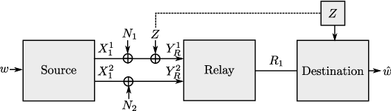
Refer to caption
Fig. 4: The parallel binary symmetric MRC-D with parallel source-relay links. The destination has side information about only one of the source-relay links.

In this section we consider a special MRC-D as shown in Figure 4, which we call the parallel binary symmetric MRC-D. For this setup, we characterize the optimal performance of the DF and CF schemes, and show that in general pDCF outperforms both, and that in some cases the cut-set bound is tight and coincides with the channel capacity. This example proves the suboptimality of both DF and CF on their own for ORC-D.

In this scenario, the source-relay channel consists of two parallel binary symmetric channels. We have X1=(X11,X12)X_{1}=(X_{1}^{1},X_{1}^{2}), YR=(YR1,YR2)Y_{R}=(Y_{R}^{1},Y_{R}^{2}) and p⁡(yR|xR,z)=p⁡(yR1|x11,z)​p​(yR2|x12)p(y_{R}|x_{R},z)=p(y_{R}^{1}|x^{1}_{1},z)p(y_{R}^{2}|x_{1}^{2}) characterized by

YR1\displaystyle Y_{R}^{1} =\displaystyle= X11⊕N1⊕Z,and YR2=X12⊕N2,\displaystyle X_{1}^{1}\oplus N_{1}\oplus Z,\quad\text{and }\quad Y_{R}^{2}=X_{1}^{2}\oplus N_{2},

where N1N_{1} and N2N_{2} are i.i.d. Bernoulli random variables with Pr{N1=1}=Pr{N2=1}=δ\text{Pr}\{N_{1}=1\}=\text{Pr}\{N_{2}=1\}=\delta, i.e., N1∼Ber​(δ)N_{1}\sim\text{Ber}(\delta) and N2∼Ber​(δ)N_{2}\sim\text{Ber}(\delta). We consider a Bernoulli distributed state ZZ, Z∼Ber​(pz)Z\sim\text{Ber}(p_{z}), which affects one of the two parallel channels, and is available at the destination. We have 𝒳11=𝒳12=𝒴R1=𝒴R1=𝒩1=𝒩2=𝒵={0,1}\mathcal{X}_{1}^{1}=\mathcal{X}_{1}^{2}=\mathcal{Y}_{R}^{1}=\mathcal{Y}_{R}^{1}=\mathcal{N}_{1}=\mathcal{N}_{2}=\mathcal{Z}=\{0,1\}.

From (11), the cut-set bound is given by

RCS\displaystyle R_{\mathrm{CS}} =\displaystyle= min⁡{R1,maxp⁡(x11​x12)⁡I⁡(X11​X12;YR1​YR2|Z)}\displaystyle\min\{R_{1},\max_{p(x_{1}^{1}x_{1}^{2})}I(X_{1}^{1}X_{1}^{2};Y_{R}^{1}Y_{R}^{2}|Z)\} (15)
=\displaystyle= min⁡{R1,2​(1−h2​(δ))},\displaystyle\min\{R_{1},2(1-h_{2}(\delta))\},

where h2​(⋅)h_{2}(\cdot) is the binary entropy function defined as h2​(p)≜−p​log⁡p−(1−p)​log⁡(1−p)h_{2}(p)\triangleq-p\log p-(1-p)\log(1-p).

The maximum DF rate is achieved by X11∼Ber​(1/2)X_{1}^{1}\sim\text{Ber}(1/2) and X12∼Ber​(1/2)X_{1}^{2}\sim\text{Ber}(1/2), and is found to be

RDF\displaystyle R_{\mathrm{DF}} =\displaystyle= min⁡{R1,maxp⁡(x11​x12)⁡I⁡(X11​X12,YR1​YR2)}\displaystyle\min\{R_{1},\max_{p(x_{1}^{1}x_{1}^{2})}I(X_{1}^{1}X_{1}^{2};Y_{R}^{1}Y_{R}^{2})\} (16)
=\displaystyle= min⁡{R1,2−h2​(δ⋆pz)−h2​(δ)},\displaystyle\min\{R_{1},2-h_{2}(\delta\star p_{z})-h_{2}(\delta)\},

where α⋆β≜α⁡(1−β)+(1−α)​β\alpha\star\beta\triangleq\alpha(1-\beta)+(1-\alpha)\beta.

Following (14), the rate achievable by the CF scheme in the parallel binary symmetric MRC-D is given by

RCF\displaystyle R_{\mathrm{CF}} =\displaystyle= max⁡I⁡(X11​X12,Y^R|Z),\displaystyle\max I(X_{1}^{1}X_{1}^{2},\hat{Y}_{R}|Z), (17)
s.t. ​R1≥I⁡(YR1​YR2;Y^R|Z)\displaystyle\text{s.t. }\;\;R_{1}\geq I(Y_{R}^{1}Y_{R}^{2};\hat{Y}_{R}|Z)
over ​p​(z)​p​(x11​x12)​p​(yR1|z,x11)​p​(yR2|x2)​p​(y^R|yR1​yR2).\displaystyle\text{over }p(z)p(x_{1}^{1}x_{1}^{2})p(y_{R}^{1}|z,x_{1}^{1})p(y_{R}^{2}|x_{2})p(\hat{y}_{R}|y_{R}^{1}y_{R}^{2}).

Let us define h2−1​(q)h_{2}^{-1}(q) as the inverse of the entropy function h2​(p)h_{2}(p) for q≥0q\geq 0. For q<0q<0, we define h2−1​(q)=0h_{2}^{-1}(q)=0.

As we show in the next lemma, the achievable CF rate in (17) is maximized by transmitting independent channel inputs over the two parallel links to the relay by setting X11∼Ber​(1/2)X_{1}^{1}\sim\text{Ber}(1/2), X12∼Ber​(1/2)X_{1}^{2}\sim\text{Ber}(1/2), and by independently compressing each of the channel outputs YR1Y_{R}^{1} and YR2Y_{R}^{2} as Y^R1=YR1⊕Q1\hat{Y}_{R}^{1}=Y_{R}^{1}\oplus Q_{1} and Y^R2=YR2⊕Q2\hat{Y}_{R}^{2}=Y_{R}^{2}\oplus Q_{2}, respectively, where Q1∼Ber​(h2−1​(1−R1/2))Q_{1}\sim\text{Ber}(h_{2}^{-1}(1-R_{1}/2)) and Q2∼Ber​(h2−1​(1−R1/2))Q_{2}\sim\text{Ber}(h_{2}^{-1}(1-R_{1}/2)). Note that for R1≥2R_{1}\geq 2, the channel outputs can be compressed errorlessly. The maximum achievable CF rate is given in the following lemma.

Lemma 4.

The maximum rate achievable by CF over the parallel binary symmetric MRC-D is given by

RCF=2​(1−h2​(δ⋆h2−1​(1−R12))).\displaystyle R_{\mathrm{CF}}=2\left(1-h_{2}\left(\delta\star h_{2}^{-1}\left(1-\frac{R_{1}}{2}\right)\right)\right). (18)
Proof.

See Appendix D. ∎

Now, we consider the pDCF scheme for the parallel binary symmetric MRC-D. Although we have not been able to characterize the optimal choice of (U,Y^R,X11,X12)(U,\hat{Y}_{R},X_{1}^{1},X_{1}^{2}) in general, we provide an achievable scheme that outperforms both DF and CF schemes and meets the cut-set bound in some regimes. Let X11∼Ber​(1/2)X_{1}^{1}\sim\text{Ber}(1/2) and X12∼Ber​(1/2)X_{1}^{2}\sim\text{Ber}(1/2) and U=X12U=X_{1}^{2}, i.e., the relay decodes the channel input X12X_{1}^{2}, while YR1Y_{R}^{1} is compressed using Y^R=YR1+Q\hat{Y}_{R}=Y_{R}^{1}+Q, where Q∼Ber​(h2−1​(2−h2​(δ)−R1))Q\sim\text{Ber}(h^{-1}_{2}(2-h_{2}(\delta)-R_{1})). The rate achievable by this scheme is given in the following lemma.

Lemma 5.

A lower bound on the achievable pDCF rate over the parallel binary symmetric MRC-D is given by

RpDCF≥min⁡{R1,2−h2​(δ)−h2​(δ⋆h2−1​(2−h2​(δ)−R1))}.\displaystyle R_{\mathrm{pDCF}}\geq\min\{R_{1},2-h_{2}(\delta)\!-\!h_{2}\left(\delta\star h_{2}^{-1}\left(2-h_{2}(\delta)\!-\!R_{1}\right)\right)\}.
Proof.

See Appendix E. ∎

Refer to caption
Fig. 5: Achievable rates and the cut-set upper bound for the parallel binary symmetric MRC-D with respect to the binary noise parameter δ\delta, for R1=1.2R_{1}=1.2 and pz=0.15p_{z}=0.15.

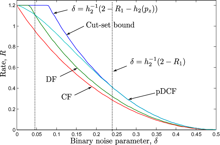
We notice that for pz≤h2−1​(2−h2​(δ)−R1)p_{z}\leq h_{2}^{-1}\left(2-h_{2}(\delta)-R_{1}\right), or equivalently, δ≤h2−1​(2−h2​(pz)−R1)\delta\leq h_{2}^{-1}\left(2-h_{2}(p_{z})-R_{1}\right), the proposed pDCF is outperformed by DF. In this regime, pDCF can achieve the same performance by decoding both channel inputs, reducing to DF.

Comparing the cut-set bound expression in (15) with RDFR_{\mathrm{DF}} in (16) and RCFR_{\mathrm{CF}} in (18), we observe that DF achieves the cut-set bound if R1≤2−h⁡(δ⋆pz)−h⁡(δ)R_{1}\leq 2-h(\delta\star p_{z})-h(\delta) while RCFR_{\mathrm{CF}} coincides with the cut-set bound if R1≥2R_{1}\geq 2. On the other hand, the proposed suboptimal pDCF scheme achieves the cut-set bound if R1≥2−h2​(δ)R_{1}\geq 2-h_{2}(\delta), i.e., for δ≥h2−1​(2−R1)\delta\geq h^{-1}_{2}(2-R_{1}). Hence, the capacity of the parallel binary symmetric MRC-D in this regime is achieved by pDCF, while both DF and CF are suboptimal, as stated in the next lemma.

Lemma 6.

If R1<2R_{1}<2 and δ≥h2−1​(2−R1)\delta\geq h^{-1}_{2}(2-R_{1}), pDCF achieves the capacity of the parallel binary symmetric MRC-D, while pure CF and DF are both suboptimal under these constraints. For R1≥2R_{1}\geq 2, both CF and pDCF achieve the capacity.

The achievable rates of DF, CF and pDCF, together with the cut-set bound are shown in Figure 5 with respect to δ\delta for R1=1.2R_{1}=1.2 and pz=0.15p_{z}=0.15. We observe that in this setup, DF outperforms CF in general, while for δ≤h2−1​(2−R1−h2​(pz))=0.0463\delta\leq h^{-1}_{2}(2-R_{1}-h_{2}(p_{z}))=0.0463, DF outperforms the proposed suboptimal pDCF scheme as well. We also observe that pDCF meets the cut-set bound for δ≥h2−1​(2−R1)=0.2430\delta\geq h^{-1}_{2}(2-R_{1})=0.2430, characterizing the capacity in this regime, and proving the suboptimality of both the DF and CF schemes when they are used on their own.

IV-B Multihop Binary Symmetric Channel

In order to gain further insights into the proposed pDCF scheme, we look into the binary symmetric MRC-D, in which, there is only a single channel connecting the source to the relay, given by

YR=X1⊕N⊕Z,\displaystyle Y_{R}=X_{1}\oplus N\oplus Z, (19)

where N∼Ber​(δ)N\sim\text{Ber}(\delta) and Z∼Ber​(pz)Z\sim\text{Ber}(p_{z}).

Similarly to Section IV-A, the cut-set bound and the maximum achievable rates for DF and CF are found as

RCS\displaystyle R_{\mathrm{CS}} =\displaystyle= min⁡{R1,1−h2​(δ)},\displaystyle\min\{R_{1},1-h_{2}(\delta)\}, (20)
RDF\displaystyle R_{\mathrm{DF}} =\displaystyle= min⁡{R1,1−h2​(δ⋆pz)},\displaystyle\min\{R_{1},1-h_{2}(\delta\star p_{z})\}, (21)
RCF\displaystyle R_{\mathrm{CF}} =\displaystyle= OPEN1−h2​(δ⋆h2−1​(1−R1))),\displaystyle 1-h_{2}(\delta\star h_{2}^{-1}(1-R_{1}))), (22)

where RDFR_{\mathrm{DF}} is achieved by X1∼Ber​(1/2)X_{1}\sim\text{Ber}(1/2), and RCFR_{\mathrm{CF}} can be shown to be maximized by X1∼Ber​(1/2)X_{1}\sim\text{Ber}(1/2) and Y^R=YR⊕Q\hat{Y}_{R}=Y_{R}\oplus Q, where Q∼Ber​(h2−1​(1−R1))Q\sim\text{Ber}(h_{2}^{-1}(1-R_{1})) similarly to Lemma 4. Note that, for YRY_{R} independent of ZZ, i.e., pz=0p_{z}=0, DF achieves the cut-set bound while CF is suboptimal. However, CF outperforms DF whenever pz≥h2−1​(1−R1)p_{z}\geq h_{2}^{-1}(1-R_{1}).

For the pDCF scheme, we consider binary (U,X1,Y^R)(U,X_{1},\hat{Y}_{R}), with U∼Ber​(p)U\sim\text{Ber}(p), a superposition codebook X1=U⊕WX_{1}=U\oplus W, where W∼Ber​(q)W\sim\text{Ber}(q), and Y^R=YR⊕Q\hat{Y}_{R}=Y_{R}\oplus Q with Q∼Ber​(α)Q\sim\text{Ber}(\alpha). As stated in the next lemma, the maximum achievable rate of this pDCF scheme is obtained by reducing it to either DF or CF, depending on the values of pzp_{z} and R1R_{1}.

Lemma 7.

For the binary symmetric MRC-D, pDCF with binary (U,X1,Y^R)(U,X_{1},\hat{Y}_{R}) achieves the following rate.

RpDCF\displaystyle R_{\mathrm{pDCF}} =\displaystyle= max⁡{RDF,RCF}\displaystyle\max\{R_{\mathrm{DF}},R_{\mathrm{CF}}\} (23)
=\displaystyle= {min⁡{R1,1−h2​(δ⋆pz)}if ​pz<h2−1​(1−R1),1−h2​(δ⋆h2−1​(1−R1))if pz≥h2−1(1−R1).\displaystyle\!\begin{cases}\min\{R_{1},1-h_{2}(\delta\star p_{z})\}&\text{if }p_{z}<h_{2}^{-1}(1-R_{1}),\\ 1-h_{2}(\delta\star h_{2}^{-1}(1-R_{1}))&\text{if }p_{z}\geq h_{2}^{-1}(1-R_{1}).\end{cases}

This result justifies the pDCF scheme proposed in Section IV-A for the parallel binary symmetric MRC-D. Since the channel p⁡(y12|x2)p(y_{1}^{2}|x_{2}) is independent of the channel state ZZ, the largest rate is are achieved if the relay decodes X12X_{1}^{2} from YR2Y_{R}^{2}. However, for channel p⁡(y11|x1,z)p(y_{1}^{1}|x_{1},z), which depends on ZZ, the relay either decodes X11X_{1}^{1}, or compress YR1Y_{R}^{1}, depending on pzp_{z}.

IV-C Multihop Gaussian Channel with State

Next, we consider an AWGN multihop channel, called Gaussian MRC-D, in which the source-relay link is characterized by YR=X1+VY_{R}=X_{1}+V, while the destination has access to correlated state information ZZ. We assume that VV and ZZ are zero-mean jointly Gaussian random variables with a covariance matrix

𝐂Z​V=[1ρρ1].\displaystyle\mathbf{C}_{ZV}=\left[\begin{matrix}1&\rho\\ \rho&1\end{matrix}\right]. (24)

The channel input at the source has to satisfy the power constraint E⁡[|X1n|2]≤n​PE[|X_{1}^{n}|^{2}]\leq nP. Finally, the relay and the destination are connected by a noiseless link of rate R1R_{1} (see Figure 6 for the channel model).

Refer to caption
Fig. 6: The multihop Gaussian relay channel with source-relay channel state information available at the destination.

In this case, the cut-set bound is given by

RCS=min⁡{R1,12​log⁡(1+P1−ρ2)}.\displaystyle R_{\mathrm{CS}}=\min\left\{R_{1},\frac{1}{2}\log\left(1+\frac{P}{1-\rho^{2}}\right)\right\}. (25)

It easy to characterize the optimal DF rate, achieved by a Gaussian input, as follows:

RDF=min⁡{R1,12​log⁡(1+P)}.\displaystyle R_{\mathrm{DF}}=\min\left\{R_{1},\frac{1}{2}\log(1+P)\right\}. (26)

For CF and pDCF, we consider the achievable rate when the random variables (X1,U,Y^R)(X_{1},U,\hat{Y}_{R}) are constrained to be jointly Gaussian, which is a common assumption in evaluating achievable rates, yet potentially suboptimal. For CF, we generate the compression codebook using Y^R=YR+Q\hat{Y}_{R}=Y_{R}+Q, where Q∼𝒩⁡(0,σq2)Q\sim\mathcal{N}(0,\sigma^{2}_{q}). Optimizing over σq2\sigma^{2}_{q}, the maximum achievable rate is given by

RCF\displaystyle R_{\mathrm{CF}} =\displaystyle= R1−12​log⁡(P+22​R1​(1−ρ2)P+1−ρ2).\displaystyle R_{1}-\frac{1}{2}\log\left(\frac{P+2^{2R_{1}}(1-\rho^{2})}{P+1-\rho^{2}}\right). (27)

For pDCF, we let U∼𝒩⁡(0,α​P1)U\sim\mathcal{N}(0,\alpha P_{1}), and X1=U+TX_{1}=U+T to be a superposition codebook where TT is independent of UU and distributed as T∼𝒩⁡(0,α¯​P1)T\sim\mathcal{N}(0,\bar{\alpha}P_{1}), where α¯≜1−α\bar{\alpha}\triangleq 1-\alpha. We generate a quantization codebook using the test channel Y^R=YR+Q\hat{Y}_{R}=Y_{R}+Q as in CF. Next lemma shows that with this choice of random variables, pDCF reduces either to pure DF or pure CF, similarly to the multihop binary model in Section IV-B.

Lemma 8.

The optimal achievable rate for pDCF with jointly Gaussian (X1,U,Y^R)(X_{1},U,\hat{Y}_{R}) is given by

RpDCF=max⁡{RDF,RCF}\displaystyle R_{\mathrm{pDCF}}=\max\{R_{\mathrm{DF}},R_{\mathrm{CF}}\} (28)
={min⁡{R1,1/2​log⁡(1+P)}if ​ρ2≤2−2​R1​(1+P),R1−12​log⁡(P+22​R1​(1−ρ2)P+1−ρ2)if ρ2>2−2​R1(1+P).\displaystyle=\begin{cases}\min\left\{R_{1},1/2\log(1+P)\right\}&\text{if }\rho^{2}\leq 2^{-2R_{1}}(1+P),\\ R_{1}-\frac{1}{2}\log\left(\frac{P+2^{2R_{1}}(1-\rho^{2})}{P+1-\rho^{2}}\right)&\text{if }\rho^{2}>2^{-2R_{1}}(1+P).\end{cases}
Proof.

See Appendix F. ∎

Refer to caption
Fig. 7: Achievable rates and the cut-set upper bound for the multihop AWGN relay channel with source-relay channel state information at the destination for R1=1R_{1}=1 and P=0.3P=0.3.

In Figure 7 the achievable rates are compared with the cut-set bound. It is shown that DF achieves the best rate when the correlation coefficient ρ\rho is low, i.e., when the destination has low quality channel state information, while CF achieves higher rates for higher values of ρ\rho. It is seen that pDCF achieves the best of the two transmission schemes. Note also that for ρ=0\rho=0 DF meets the cut-set bound, while for ρ=1\rho=1 CF meets the cut-set bound.

Although this example proves the suboptimality of the DF scheme for the channel model under consideration, it does not necessarily lead to the suboptimality of the CF scheme as we have constrained the auxiliary random variables to be Gaussian.

V Comparison with the Cut-Set Bound

In the examples considered in Section IV, we have seen that for certain conditions, the choice of certain random variables allows us to show that the cut-set bound and the capacity coincide. For example, we have seen that for the parallel binary symmetric MRC-D the proposed pDCF scheme achieves the cut-set bound for δ≥h2−1​(2−R1)\delta\geq h^{-1}_{2}(2-R_{1}), or Gaussian random variables meet the cut-set bound for ρ=0\rho=0 or ρ=1\rho=1 in the Gaussian MRC-D. An interesting question is whether the capacity expression in Theorem 1 always coincides with the cut-set bound or not; that is, whether the cut-set bound is tight for the relay channel model under consideration.

To address this question, we consider the multihop binary channel in (19) for Z∼Ber​(1/2)Z\sim\text{Ber}(1/2). The capacity 𝒞\mathcal{C} of this channel is given in the following lemma.

Lemma 9.

The capacity of the binary symmetric MRC-D with YR=X1⊕N⊕ZY_{R}=X_{1}\oplus N\oplus Z, where N∼Ber​(δ)N\sim\text{Ber}(\delta) and Z∼Ber​(1/2)Z\sim\text{Ber}(1/2), is achieved by CF and pDCF, and is given by

𝒞=1−h2​(δ⋆h2−1​(1−R1)).\displaystyle\mathcal{C}=1-h_{2}(\delta\star h_{2}^{-1}(1-R_{1})). (29)
Proof.

See Appendix G. ∎

From (20), the cut-set bound is given by RCS=1−h2​(δ)R_{\mathrm{CS}}=1-h_{2}(\delta). It then follows that in general the capacity is below the cut-set bound. Note that for this setup, RDF=0R_{\mathrm{DF}}=0 and pDCF reduces to CF, i.e., RpDCF=RCFR_{\mathrm{pDCF}}=R_{\mathrm{CF}}. See Figure 8 for comparison of the capacity with the cut-set bound for varying δ\delta values.

CF suffices to achieve the capacity of the binary symmetric MRC-D for Z∼Ber​(1/2)Z\sim\text{Ber}(1/2). While in general pDCF outperforms DF and CF, in certain cases these two schemes are sufficient to achieve the cut-set bound, and hence, the capacity. For the ORC-D model introduced in Section II, the cut-set bound is given by

RCS=R2+min⁡{R1,maxp⁡(x1)⁡I⁡(X1;YR|Z)}.\displaystyle R_{\mathrm{CS}}=R_{2}+\min\{R_{1},\max_{p(x_{1})}I(X_{1};Y_{R}|Z)\}. (30)

Next, we present four cases for which the cut-set bound is achievable, and hence, is the capacity:

  • Case 1) If I⁡(Z,YR)=0I(Z;Y_{R})=0, the setup reduces to the class of orthogonal relay channels studied in [3], for which the capacity is known to be achieved by pDF.

  • Case 2) If H⁡(YR|X1​Z)=0H(Y_{R}|X_{1}Z)=0, i.e., YRY_{R} is a deterministic function of X1X_{1} and ZZ, the capacity, given by

    R2+min⁡{R1,maxp⁡(x1)⁡I⁡(X1;YR|Z)},R_{2}+\min\{R_{1},\max_{p(x_{1})}I(X_{1};Y_{R}|Z)\},

    is achievable by CF.

  • Case 3) If maxp⁡(x1)⁡I⁡(X1,YR)≥R1\max_{p(x_{1})}I(X_{1};Y_{R})\geq R_{1}, the capacity, given by 𝒞=R2+R1\mathcal{C}=R_{2}+R_{1}, is achievable by pDF.

  • Case 4) Let arg⁡maxp⁡(x1)⁡I⁡(X1;YR|Z)=p¯​(x1)\arg\max_{p(x_{1})}I(X_{1};Y_{R}|Z)=\bar{p}(x_{1}). If R1>H⁡(Y¯R|Z)R_{1}>H(\bar{Y}_{R}|Z) for Y¯R\bar{Y}_{R} induced by p¯​(x1)\bar{p}(x_{1}), the capacity, given by R2+I⁡(X¯1;Y¯R|Z)R_{2}+I(\bar{X}_{1};\bar{Y}_{R}|Z), is achievable by CF.

Proof.

See Appendix H. ∎

Refer to caption
Fig. 8: Achievable rates, capacity and cut-set upper bound for the multihop binary relay channel with respect to δ\delta for R1=0.25R_{1}=0.25 and pz=0.5p_{z}=0.5.

These cases can be observed in the examples from Section IV. For example, in the Gaussian MRC-D with ρ=0\rho=0, YRY_{R} is independent of ZZ, and thus, DF meets the cut-set bound as stated in Case 1. Similarly, for ρ=1\rho=1 CF meets the cut-set bound since YRY_{R} is a deterministic function of XRX_{R} and ZZ, which corresponds to Case 2.

For the parallel binary symmetric MRC-D in Section IV-A, pDCF achieves the cut-set bound if δ≥h2−1​(2−R1)\delta\geq h^{-1}_{2}(2-R_{1}) due to the following reasoning. Since YR1Y_{R}^{1} is independent of X11X_{1}^{1}, from Case 1, DF should achieve the cut-set bound. Once X11X_{1}^{1} is decoded, the available rate to compress Y2Y_{2} is given by R1−I⁡(X1,Y1)=R1−1+h2​(δ)R_{1}-I(X_{1};Y_{1})=R_{1}-1+h_{2}(\delta), and the entropy of Y2Y_{2} conditioned on the channel state at the destination is given by H⁡(Y2|Z)=1−h2​(δ)H(Y_{2}|Z)=1-h_{2}(\delta). For δ≥h2−1​(2−R1)\delta\geq h^{-1}_{2}(2-R_{1}) we have R1−I⁡(X1,Y1)≥H⁡(Y2|Z)R_{1}-I(X_{1};Y_{1})\geq H(Y_{2}|Z). Therefore the relay can compress Y2Y_{2} losslessly, and transmit to the destination. This corresponds to Case 4. Thus, the capacity characterization in the parallel binary symmetric MRC-D is due to a combination of Case 1 and Case 4.

VI Conclusion

We have considered a class of orthogonal relay channels, in which the channels connecting the source to the relay and the destination, and the relay to the destination, depend on a state sequence, known at the destination. We have characterized the capacity of this class of relay channels, and shown that it is achieved by the partial decode-compress-and-forward (pDCF) scheme. This is the first three-terminal relay channel model for which the pDCF is shown to be capacity achieving while partial decode-and-forward (pDF) and compress-and-forward (CF) schemes are both suboptimal in general. We have also shown that, in general, the capacity of this channel is below the cut-set bound.

Appendix A Proof of Lemma 1

In the rate expression and joint pmf in Theorem 2, we set Xn=(X1n,X2n)X^{n}=(X_{1}^{n},X_{2}^{n}), Yn=(Y1n,Y2n,Zn)Y^{n}=(Y_{1}^{n},Y_{2}^{n},Z^{n}), V=∅V=\emptyset, and generate XRnX_{R}^{n} and X2nX_{2}^{n} independent of the rest of the random variables with distributions p∗​(xR)p^{*}(x_{R}) and p∗​(x2)p^{*}(x_{2}), which maximize the mutual information terms in (5), respectively. Under this set of distributions we have

I⁡(X;Y​Y^R|XR​U)\displaystyle I(X;Y\hat{Y}_{R}|X_{R}U) =\displaystyle= I(X1X2;Y1Y2Y^RZ|XR,U)\displaystyle I(X_{1}X_{2};Y_{1}Y_{2}\hat{Y}_{R}Z|X_{R},U)
=(a)\displaystyle\stackrel{{\scriptstyle(a)}}{{=}} I⁡(X1​X2;Y2​Y^R|XR​U​Z)\displaystyle I(X_{1}X_{2};Y_{2}\hat{Y}_{R}|X_{R}UZ)
=(b)\displaystyle\stackrel{{\scriptstyle(b)}}{{=}} I⁡(X2;Y2|Z)+I⁡(X1;Y^R|U​Z)\displaystyle I(X_{2};Y_{2}|Z)+I(X_{1};\hat{Y}_{R}|UZ)
=\displaystyle= R2+I⁡(X1;Y^R|U​Z),\displaystyle R_{2}+I(X_{1};\hat{Y}_{R}|UZ),
I⁡(U;YR|XR​V)\displaystyle I(U;Y_{R}|X_{R}V) =\displaystyle= I⁡(U;YR|XR)=(c)I⁡(U,YR),\displaystyle I(U;Y_{R}|X_{R})\stackrel{{\scriptstyle(c)}}{{=}}I(U;Y_{R}),
I⁡(X​XR,Y)\displaystyle I(XX_{R};Y) =\displaystyle= I⁡(X1​X2​XR,Y1​Y2​Z)\displaystyle I(X_{1}X_{2}X_{R};Y_{1}Y_{2}Z)
=(d)\displaystyle\stackrel{{\scriptstyle(d)}}{{=}} I⁡(X2​XR;Y1​Y2|Z)\displaystyle I(X_{2}X_{R};Y_{1}Y_{2}|Z)
=(e)\displaystyle\stackrel{{\scriptstyle(e)}}{{=}} I⁡(XR,Y1)+I⁡(X2;Y2|Z)=R1+R2,\displaystyle I(X_{R};Y_{1})+I(X_{2};Y_{2}|Z)=R_{1}+R_{2},
I⁡(Y^R;YR|X​XR​U​Y)\displaystyle I(\hat{Y}_{R};Y_{R}|XX_{R}UY) =\displaystyle= I⁡(Y^R;YR|XR​X1​X2​U​Y1​Y2​Z)\displaystyle I(\hat{Y}_{R};Y_{R}|X_{R}X_{1}X_{2}UY_{1}Y_{2}Z)
=(f)\displaystyle\stackrel{{\scriptstyle(f)}}{{=}} I⁡(Y^R;YR|XR​X1​X2​U​Y2​Z)\displaystyle I(\hat{Y}_{R};Y_{R}|X_{R}X_{1}X_{2}UY_{2}Z)
=(g)\displaystyle\stackrel{{\scriptstyle(g)}}{{=}} I⁡(Y^R;YR|X1​U​Z),\displaystyle I(\hat{Y}_{R};Y_{R}|X_{1}UZ),
I⁡(Y^R;YR|Y​XR​U)\displaystyle I(\hat{Y}_{R};Y_{R}|YX_{R}U) =\displaystyle= I⁡(Y^R;YR|Y1​Y2​Z​XR​U)\displaystyle I(\hat{Y}_{R};Y_{R}|Y_{1}Y_{2}ZX_{R}U)
=(h)\displaystyle\stackrel{{\scriptstyle(h)}}{{=}} I⁡(Y^R;YR|U​Z),\displaystyle I(\hat{Y}_{R};Y_{R}|UZ),
I⁡(XR;Y|V)\displaystyle I(X_{R};Y|V) =\displaystyle= I⁡(XR,Y1​Y2​Z)=I⁡(XR,Y1)=R1,\displaystyle I(X_{R};Y_{1}Y_{2}Z)=I(X_{R};Y_{1})=R_{1},

where (a)(a) is due to the Markov chain (X1​X2)−XR−Y1(X_{1}X_{2})-X_{R}-Y_{1}; (b),(c),(e),(f),(g),(h)(b),(c),(e),(f),(g),(h) are due to the independence of (U,X1)(U,X_{1}) and XRX_{R}, and (d)(d) is due to the Markov chain (Y1​Y2)−(X2​XR​Z)−X1(Y_{1}Y_{2})-(X_{2}X_{R}Z)-X_{1}.

Then, (8) reduces to the following rate

R=\displaystyle R= sup𝒫\displaystyle\underset{\mathcal{P}}{\sup} min{I(U;YR)+R2+I(X1;Y^R|UZ),\displaystyle\,\min\{I(U;Y_{R})+R_{2}+I(X_{1};\hat{Y}_{R}|UZ), (31)
R2+R1−I(Y^R;YR|X1UZ)},\displaystyle\;\qquad R_{2}+R_{1}-I(\hat{Y}_{R};Y_{R}|X_{1}UZ)\},
s.t. R1≥I⁡(Y^R;YR|U​Z).\displaystyle R_{1}\geq I(\hat{Y}_{R};Y_{R}|UZ). (32)

Focusing on the joint distributions in 𝒫\mathcal{P} such that the minimum in RR is achieved for the first argument, i.e.,

R1−I⁡(Y^R;YR|X1​U​Z)≥I⁡(U,YR)+I⁡(X1;Y^R|U​Z),\displaystyle R_{1}-I(\hat{Y}_{R};Y_{R}|X_{1}UZ)\geq I(U;Y_{R})+I(X_{1};\hat{Y}_{R}|UZ),

and using the chain rule for the mutual information, the rate achievable by pDCF is lower bounded by

R≥\displaystyle R\geq sup𝒫\displaystyle\underset{\mathcal{P}}{\sup}\; R2+I⁡(U,YR)+I⁡(X1;Y^R|U​Z)\displaystyle R_{2}+I(U;Y_{R})+I(X_{1};\hat{Y}_{R}|UZ) (33)
s.t. R1≥I⁡(U,YR)+I⁡(X1​YR;Y^R|U​Z),\displaystyle R_{1}\geq I(U;Y_{R})+I(X_{1}Y_{R};\hat{Y}_{R}|UZ),
R1≥I⁡(Y^R;YR|U​Z).\displaystyle R_{1}\geq I(\hat{Y}_{R};Y_{R}|UZ). (34)

From (33), we have

R1\displaystyle R_{1} ≥\displaystyle\geq I⁡(U,YR)+I⁡(X1​YR;Y^R|U​Z)\displaystyle I(U;Y_{R})+I(X_{1}Y_{R};\hat{Y}_{R}|UZ) (35)
=(a)\displaystyle\stackrel{{\scriptstyle(a)}}{{=}} I⁡(U,YR)+I⁡(Y^R;YR|U​Z)\displaystyle I(U;Y_{R})+I(\hat{Y}_{R};Y_{R}|UZ)
≥\displaystyle\geq I⁡(Y^R;YR|U​Z),\displaystyle I(\hat{Y}_{R};Y_{R}|UZ),

where (a)(a) is due to the Markov chain Y^R−(U​YR)−(X1​Z)\hat{Y}_{R}-(UY_{R})-(X_{1}Z). Hence, (33) implies (34), i.e., the latter condition is redundant, and R≥𝒞R\geq\mathcal{C}. Therefore the capacity expression 𝒞\mathcal{C} in (7) is achievable by pDCF. This concludes the proof.

Appendix B Proof of Lemma 2

Consider any sequence of (2n​R,n,νn)(2^{nR},n,\nu_{n}) codes such that limn→∞νn→0\lim_{n\rightarrow\infty}\nu_{n}\rightarrow 0. We need to show that R≤Ru​pR\leq R_{up}.

Let us define Ui≜(YR​1i−1​X1​i+1n​Zn∖i)U_{i}\triangleq(Y_{R1}^{i-1}X_{1i+1}^{n}Z^{n\setminus i}) and Y^R​i≜(Y1​i+1n)\hat{Y}_{Ri}\triangleq(Y_{1i+1}^{n}). For such Y^R​i\hat{Y}_{Ri} and UiU_{i}, the following Markov chain holds

Y^R​i−(Ui,YR​i)−(X1​i,X2​i,Zi,Y1​i,Y2​i,XR​i).\displaystyle\hat{Y}_{Ri}-(U_{i},Y_{Ri})-(X_{1i},X_{2i},Z_{i},Y_{1i},Y_{2i},X_{Ri}). (36)

From Fano’s inequality, we have

H⁡(W|Y1n​Y2n​Zn)≤n​ϵn,\displaystyle H(W|Y_{1}^{n}Y_{2}^{n}Z^{n})\leq n\epsilon_{n}, (37)

such that ϵn→0\epsilon_{n}\rightarrow 0 as n→∞n\rightarrow\infty.

First, we derive the following set of inequalities related to the capacity of the source-destination channel.

n​R\displaystyle nR =\displaystyle= H⁡(W)\displaystyle H(W) (38)
=(a)\displaystyle\stackrel{{\scriptstyle(a)}}{{=}} I⁡(W;Y1n​Y2n|Zn)+H⁡(W|Y1n​Y2n​Zn)\displaystyle I(W;Y_{1}^{n}Y_{2}^{n}|Z^{n})+H(W|Y_{1}^{n}Y_{2}^{n}Z^{n})
≤(b)\displaystyle\stackrel{{\scriptstyle(b)}}{{\leq}} I⁡(X1n​X2n;Y1n​Y2n|Zn)+n​ϵn,\displaystyle I(X_{1}^{n}X_{2}^{n};Y_{1}^{n}Y_{2}^{n}|Z^{n})+n\epsilon_{n},

where (a)(a) follows from the independence of ZnZ^{n} and WW; and (b)(b) follows from Fano’s inequality in (37).

We also have the following inequalities:

I⁡(X2n;Y2n|Zn)\displaystyle I(X_{2}^{n};Y_{2}^{n}|Z^{n})\! =\displaystyle= ∑i=1nH⁡(Y2​i|Zn​Y21i−1)−H⁡(Y2​i|Zn​Y21i−1​X2n)\displaystyle\!\sum_{i=1}^{n}H(Y_{2i}|Z^{n}Y_{21}^{i-1})-H(Y_{2i}|Z^{n}Y_{21}^{i-1}X_{2}^{n}) (39)
≤(a)\displaystyle\stackrel{{\scriptstyle(a)}}{{\leq}} ∑i=1nH⁡(Y2​i|Zi)−H⁡(Y2​i|Zi​X2​i)\displaystyle\sum_{i=1}^{n}H(Y_{2i}|Z_{i})-H(Y_{2i}|Z_{i}X_{2i})
=\displaystyle= ∑i=1nI⁡(X2​i;Y2​i|Zi)\displaystyle\sum_{i=1}^{n}I(X_{2i};Y_{2i}|Z_{i})
=(b)\displaystyle\stackrel{{\scriptstyle(b)}}{{=}} n​I​(X2​Q′;Y2​Q′|ZQ′​Q′)\displaystyle nI(X_{2Q^{\prime}};Y_{2Q^{\prime}}|Z_{Q^{\prime}}Q^{\prime})
≤(c)\displaystyle\stackrel{{\scriptstyle(c)}}{{\leq}} n​I​(X2​Q′;Y2​Q′|ZQ′)\displaystyle nI(X_{2Q^{\prime}};Y_{2Q^{\prime}}|Z_{Q^{\prime}})
≤(d)\displaystyle\stackrel{{\scriptstyle(d)}}{{\leq}} n​R2,\displaystyle nR_{2},

where (a)(a) follows since conditioning reduces entropy, (b)(b) follows by defining Q′Q^{\prime} as a uniformly distributed random variable over {1,…,n}\{1,...,n\} and (X2​Q′,Y2​Q′,ZQ′)(X_{2Q^{\prime}},Y_{2Q^{\prime}},Z_{Q^{\prime}}) as a pair of random variables satisfying Pr{X2​i=x2,Y2​i=y2,Zi=z}=Pr{X2​Q′=x2,Y2​Q′=y2,,ZQ′=z|Q=i}\text{Pr}\{X_{2i}=x_{2},Y_{2i}=y_{2},Z_{i}=z\}=\text{Pr}\{X_{2Q^{\prime}}=x_{2},Y_{2Q^{\prime}}=y_{2},,Z_{Q^{\prime}}=z|Q=i\} for i=1,…,ni=1,...,n, (c)(c) follows from the Markov chain relation Q′−X2​Q′−Y2​Q′Q^{\prime}-X_{2Q^{\prime}}-Y_{2Q^{\prime}} and (d)(d) follows from the definition of R2R_{2} in (5). Following the same steps, we obtain

I⁡(XRn;Y1n|Zn)≤n​R1.\displaystyle I(X_{R}^{n};Y_{1}^{n}|Z^{n})\leq nR_{1}. (40)

Then, we can bound the achievable rate as,

n​R\displaystyle nR =\displaystyle= I⁡(W,Y1n​Y2n​Zn)+H⁡(W|Y1n​Y2n​Zn)\displaystyle I(W;Y_{1}^{n}Y_{2}^{n}Z^{n})+H(W|Y_{1}^{n}Y_{2}^{n}Z^{n})
≤(a)\displaystyle\stackrel{{\scriptstyle(a)}}{{\leq}} I⁡(W,Y1n​Y2n​Zn)+n​ϵn\displaystyle I(W;Y_{1}^{n}Y_{2}^{n}Z^{n})+n\epsilon_{n}
=(b)\displaystyle\stackrel{{\scriptstyle(b)}}{{=}} I⁡(W;Y2n|Zn)+I⁡(W;Y1n|Y2n​Zn)+n​ϵn\displaystyle I(W;Y_{2}^{n}|Z^{n})+I(W;Y_{1}^{n}|Y_{2}^{n}Z^{n})+n\epsilon_{n}
≤(c)\displaystyle\stackrel{{\scriptstyle(c)}}{{\leq}} I⁡(X2n;Y2n|Zn)+I⁡(W;Y1n|Y2n​Zn)+n​ϵn\displaystyle I(X_{2}^{n};Y_{2}^{n}|Z^{n})+I(W;Y_{1}^{n}|Y_{2}^{n}Z^{n})+n\epsilon_{n}
≤(d)\displaystyle\stackrel{{\scriptstyle(d)}}{{\leq}} n​R2+H⁡(Y1n|Y2n​Zn)−H⁡(Y1n|W​Zn)+n​ϵn\displaystyle nR_{2}+H(Y_{1}^{n}|Y_{2}^{n}Z^{n})-H(Y_{1}^{n}|WZ^{n})+n\epsilon_{n}
≤(e)\displaystyle\stackrel{{\scriptstyle(e)}}{{\leq}} n​R2+H⁡(Y1n|Zn)−H⁡(Y1n|W​X1n​Zn)+n​ϵn\displaystyle nR_{2}+H(Y_{1}^{n}|Z^{n})-H(Y_{1}^{n}|WX_{1}^{n}Z^{n})+n\epsilon_{n}
=(f)\displaystyle\stackrel{{\scriptstyle(f)}}{{=}} n​R2+I⁡(X1n;Y1n|Zn)+n​ϵn\displaystyle nR_{2}+I(X_{1}^{n};Y_{1}^{n}|Z^{n})+n\epsilon_{n}
≤(g)\displaystyle\stackrel{{\scriptstyle(g)}}{{\leq}} n​R2+H⁡(X1n)−H⁡(X1n|Y1n​Zn)+n​ϵn\displaystyle nR_{2}+H(X_{1}^{n})-H(X_{1}^{n}|Y_{1}^{n}Z^{n})+n\epsilon_{n}
=\displaystyle= n​R2+∑i=1nH⁡(X1​i|X1​i+1n)−H⁡(X1n|Y1n​Zn)+n​ϵn\displaystyle nR_{2}+\sum_{i=1}^{n}H(X_{1i}|X_{1i+1}^{n})-H(X_{1}^{n}|Y_{1}^{n}Z^{n})+n\epsilon_{n}
≤(h)\displaystyle\stackrel{{\scriptstyle(h)}}{{\leq}} nR2+∑i=1n[I(YR​1i−1Zn∖i;YR​i)\displaystyle nR_{2}+\sum_{i=1}^{n}\bigg[I(Y_{R1}^{i-1}Z^{n\setminus i};Y_{Ri})
+H(X1​i|X1​i+1n)]−H(X1n|Y1nZn)+nϵn\displaystyle+H(X_{1i}|X_{1i+1}^{n})\bigg]-H(X_{1}^{n}|Y_{1}^{n}Z^{n})+n\epsilon_{n}
=\displaystyle= nR2+∑i=1n[I(YR​1i−1Zn∖iX1​i+1n;YR​i)\displaystyle nR_{2}+\sum_{i=1}^{n}\bigg[I(Y_{R1}^{i-1}Z^{n\setminus i}X_{1i+1}^{n};Y_{Ri})
−I⁡(X1​i+1n;YR​i|YR​1i−1​Zn∖i)+H⁡(X1​i|YR​1i−1​Zn∖i​X1​i+1n)\displaystyle-I(X_{1i+1}^{n};Y_{Ri}|Y_{R1}^{i-1}Z^{n\setminus i})+H(X_{1i}|Y_{R1}^{i-1}Z^{n\setminus i}X_{1i+1}^{n})
+I(X1​i;YR​1i−1Zn∖i|X1​i+1n)]−H(X1n|Y1nZn)+nϵn\displaystyle+I(X_{1i};Y_{R1}^{i-1}Z^{n\setminus i}|X_{1i+1}^{n})\bigg]-H(X_{1}^{n}|Y_{1}^{n}Z^{n})+n\epsilon_{n}
=(i)\displaystyle\stackrel{{\scriptstyle(i)}}{{=}} nR2+∑i=1n[I(YR​1i−1Zn∖iX1​i+1n;YR​i)\displaystyle nR_{2}+\sum_{i=1}^{n}\bigg[I(Y_{R1}^{i-1}Z^{n\setminus i}X_{1i+1}^{n};Y_{Ri})
+H(X1​i|YR​1i−1Zn∖iX1​i+1n)]−H(X1n|Y1nZn)+nϵn\displaystyle+H(X_{1i}|Y_{R1}^{i-1}Z^{n\setminus i}X_{1i+1}^{n})\bigg]-H(X_{1}^{n}|Y_{1}^{n}Z^{n})+n\epsilon_{n}
=\displaystyle= n​R2+∑i=1n[I⁡(Ui,YR​i)+H⁡(X1​i|Ui)]\displaystyle nR_{2}+\sum_{i=1}^{n}\bigg[I(U_{i};Y_{Ri})+H(X_{1i}|U_{i})\bigg]
−H⁡(X1n|Y1n​Zn)+n​ϵn\displaystyle-H(X_{1}^{n}|Y_{1}^{n}Z^{n})+n\epsilon_{n}
≤(j)\displaystyle\stackrel{{\scriptstyle(j)}}{{\leq}} nR2+∑i=1n[I(Ui;YR​i)+H(X1​i|Ui)\displaystyle nR_{2}+\sum_{i=1}^{n}\bigg[I(U_{i};Y_{Ri})+H(X_{1i}|U_{i})
−H(X1​i|UiZiY^R​i)]+nϵn\displaystyle-H(X_{1i}|U_{i}Z_{i}\hat{Y}_{Ri})\bigg]+n\epsilon_{n}
=(k)\displaystyle\stackrel{{\scriptstyle(k)}}{{=}} n​R2+∑i=1n[I⁡(Ui,YR​i)+I⁡(X1​i;Y^R​i|Ui​Zi)]+n​ϵn,\displaystyle nR_{2}+\sum_{i=1}^{n}\bigg[I(U_{i};Y_{Ri})+I(X_{1i};\hat{Y}_{Ri}|U_{i}Z_{i})\bigg]+n\epsilon_{n},

where (a)(a) is due to Fano’s inequality; (b)(b) is due to the chain rule and the independence of ZnZ^{n} from WW; (c)(c) is due to the data processing inequality; (d)(d) is due to the Markov chain relation Y2n−(W,Zn)−Y1nY_{2}^{n}-(W,Z^{n})-Y_{1}^{n} and (39); (e)(e) is due to the fact that conditioning reduces entropy, and that X1nX_{1}^{n} is a deterministic function of WW; (f)(f) is due to the Markov chain relation Y1n−X1n−WY^{n}_{1}-X_{1}^{n}-W; (g)(g) is due to the independence of ZnZ^{n} and X1nX_{1}^{n}; (i)(i) follows because

∑i=1nI⁡(X1​i;YR​1i−1​Zn∖i|X1​i+1n)\displaystyle\sum_{i=1}^{n}I(X_{1i};Y_{R1}^{i-1}Z^{n\setminus i}|X_{1i+1}^{n}) =(l)\displaystyle\stackrel{{\scriptstyle(l)}}{{=}} ∑i=1nI⁡(X1​i;YR​1i−1|X1​i+1n​Zn∖i)\displaystyle\sum_{i=1}^{n}I(X_{1i};Y_{R1}^{i-1}|X_{1i+1}^{n}Z^{n\setminus i})
=(m)\displaystyle\stackrel{{\scriptstyle(m)}}{{=}} ∑i=1nI⁡(X1​i+1n;YR​i|YR​1i−1​Zn∖i),\displaystyle\sum_{i=1}^{n}I(X_{1i+1}^{n};Y_{Ri}|Y_{R1}^{i-1}Z^{n\setminus i}),

where (l)(l) is due to the independence of ZnZ^{n} and X1nX_{1}^{n}; and (m)(m) is the conditional version of Csiszár’s equality [24]. Inequality (j)(j) is due to the following bound,

H⁡(X1n|Y1n​Zn)\displaystyle H(X_{1}^{n}|Y_{1}^{n}Z^{n}) =\displaystyle= ∑i=1nH⁡(X1​i|X1​i+1n​Zn​Y1n)\displaystyle\sum_{i=1}^{n}H(X_{1i}|X_{1i+1}^{n}Z^{n}Y_{1}^{n}) (41)
≥\displaystyle\geq ∑i=1nH⁡(X1​i|YR​1i−1​X1​i+1n​Zn​Y1n)\displaystyle\sum_{i=1}^{n}H(X_{1i}|Y_{R1}^{i-1}X_{1i+1}^{n}Z^{n}Y_{1}^{n})
=(n)\displaystyle\stackrel{{\scriptstyle(n)}}{{=}} ∑i=1nH⁡(X1​i|YR​1i−1​X1​i+1n​Zn​Y1​i+1n)\displaystyle\sum_{i=1}^{n}H(X_{1i}|Y_{R1}^{i-1}X_{1i+1}^{n}Z^{n}Y_{1i+1}^{n})
=\displaystyle= ∑i=1nH⁡(X1​i|Ui​Zi​Y^R​i),\displaystyle\sum_{i=1}^{n}H(X_{1i}|U_{i}Z_{i}\hat{Y}_{Ri}),

where (n)(n) is follows from the Markov chain relation X1​i−(YR​1i−1​X1​i+1n​Zn​Y1​i+1n)−Y11iX_{1i}-(Y_{R1}^{i-1}X_{1i+1}^{n}Z^{n}Y_{1i+1}^{n})-Y_{11}^{i}, and noticing that XR​i=fr,i​(YR​1i−1)X_{Ri}=f_{r,i}(Y_{R1}^{i-1}). Finally, (k)(k) is due to the fact that ZiZ_{i} independent of (X1​i,Ui)(X_{1i},U_{i}).

We can also obtain the following sequence of inequalities

n​R1\displaystyle nR_{1} +n​R2\displaystyle+nR_{2}
≥(a)\displaystyle\stackrel{{\scriptstyle(a)}}{{\geq}} I⁡(XRn;Y1n|Zn)+I⁡(X2n;Y2n|Zn)\displaystyle I(X_{R}^{n};Y_{1}^{n}|Z^{n})+I(X_{2}^{n};Y_{2}^{n}|Z^{n})
≥(b)\displaystyle\stackrel{{\scriptstyle(b)}}{{\geq}} H⁡(Y2n|Zn)−H⁡(Y2n|X2n​Zn)\displaystyle H(Y_{2}^{n}|Z^{n})-H(Y_{2}^{n}|X_{2}^{n}Z^{n})
+H⁡(Y1n|Y2n​Zn)−H⁡(Y1n|XRn​Zn)\displaystyle+H(Y_{1}^{n}|Y_{2}^{n}Z^{n})-H(Y_{1}^{n}|X_{R}^{n}Z^{n})
=\displaystyle= H⁡(Y1n​Y2n|Zn)−H⁡(Y2n|X2n​Zn)−H⁡(Y1n|XRn​Zn)\displaystyle H(Y_{1}^{n}Y_{2}^{n}|Z^{n})-H(Y_{2}^{n}|X_{2}^{n}Z^{n})-H(Y_{1}^{n}|X_{R}^{n}Z^{n})
=(c)\displaystyle\stackrel{{\scriptstyle(c)}}{{=}} H⁡(Y1n​Y2n|Zn)−H⁡(Y2n|X1n​X2n​YRn​Zn)\displaystyle H(Y_{1}^{n}Y_{2}^{n}|Z^{n})-H(Y_{2}^{n}|X_{1}^{n}X_{2}^{n}Y_{R}^{n}Z^{n})
−H⁡(Y1n|XRn​X1n​X2n​YRn​Y2n​Zn)\displaystyle-H(Y_{1}^{n}|X_{R}^{n}X_{1}^{n}X_{2}^{n}Y_{R}^{n}Y_{2}^{n}Z^{n})
≥(d)\displaystyle\stackrel{{\scriptstyle(d)}}{{\geq}} H⁡(Y1n​Y2n|Zn)−H⁡(Y1n​Y2n|X1n​X2n​YRn​Zn)\displaystyle H(Y_{1}^{n}Y_{2}^{n}|Z^{n})-H(Y_{1}^{n}Y_{2}^{n}|X_{1}^{n}X_{2}^{n}Y_{R}^{n}Z^{n})
=\displaystyle= I⁡(Y1n​Y2n;X1n​X2n​YRn|Zn)\displaystyle I(Y_{1}^{n}Y_{2}^{n};X_{1}^{n}X_{2}^{n}Y_{R}^{n}|Z^{n})
=\displaystyle= I⁡(X1n​X2n;Y1n​Y2n|Zn)+I⁡(Y1n​Y2n;YRn|X1n​X2n​Zn)\displaystyle I(X_{1}^{n}X_{2}^{n};Y_{1}^{n}Y_{2}^{n}|Z^{n})+I(Y_{1}^{n}Y_{2}^{n};Y_{R}^{n}|X_{1}^{n}X_{2}^{n}Z^{n})
≥(e)\displaystyle\stackrel{{\scriptstyle(e)}}{{\geq}} n​R+I⁡(Y1n​Y2n;YRn|X1n​X2n​Zn)−n​ϵn\displaystyle nR+I(Y_{1}^{n}Y_{2}^{n};Y_{R}^{n}|X_{1}^{n}X_{2}^{n}Z^{n})-n\epsilon_{n}
=(f)\displaystyle\stackrel{{\scriptstyle(f)}}{{=}} n​R+I⁡(Y1n;YRn|X1n​Zn)−n​ϵn\displaystyle nR+I(Y_{1}^{n};Y_{R}^{n}|X_{1}^{n}Z^{n})-n\epsilon_{n}
=\displaystyle= n​R+∑i=1nI⁡(Y1n;YR​i|X1n​YR​1i−1​Zn)−n​ϵn\displaystyle nR+\sum_{i=1}^{n}I(Y_{1}^{n};Y_{Ri}|X_{1}^{n}Y_{R1}^{i-1}Z^{n})-n\epsilon_{n}
≥\displaystyle\geq n​R+∑i=1nI⁡(Y1​i+1n;YR​i|X1n​YR​1i−1​Zn)−n​ϵn\displaystyle nR+\sum_{i=1}^{n}I(Y_{1i+1}^{n};Y_{Ri}|X_{1}^{n}Y_{R1}^{i-1}Z^{n})-n\epsilon_{n}
≥(g)\displaystyle\stackrel{{\scriptstyle(g)}}{{\geq}} n​R+∑i=1nI⁡(Y1​i+1n;YR​i|X1​in​YR​1i−1​Zn)−n​ϵn\displaystyle nR+\sum_{i=1}^{n}I(Y_{1i+1}^{n};Y_{Ri}|X_{1i}^{n}Y_{R1}^{i-1}Z^{n})-n\epsilon_{n}
=\displaystyle= n​R+∑i=1nI⁡(Y^R​i;YR​i|X1​i​Ui​Zi)−n​ϵn,\displaystyle nR+\sum_{i=1}^{n}I(\hat{Y}_{Ri};Y_{Ri}|X_{1i}U_{i}Z_{i})-n\epsilon_{n},

where (a)(a) follows from (39) and (40); (b)(b) is due to the fact that conditioning reduces entropy; (c)(c) is due to the Markov chains Y2n−(X2n​Zn)−(X1n​YRn)Y_{2}^{n}-(X_{2}^{n}Z^{n})-(X_{1}^{n}Y_{R}^{n}) and Y1n−(XRn​Zn)−(X1n​X2n​YRn​Y2n)Y_{1}^{n}-(X_{R}^{n}Z^{n})-(X_{1}^{n}X_{2}^{n}Y_{R}^{n}Y_{2}^{n}); (d)(d) follows since conditioning reduces entropy; (e)(e) is due to the expression in (38); (f)(f) is due to the Markov chain (YRn​Y1n)−(X1n​Zn)−(X2n​Y2n)(Y_{R}^{n}Y_{1}^{n})-(X_{1}^{n}Z^{n})-(X_{2}^{n}Y_{2}^{n}) and; (g)(g) is due to the Markov chain (Y1​i+1n)−(X1​in​YR​1i−1​Zn)−X11i−1(Y_{1i+1}^{n})-(X_{1i}^{n}Y_{R1}^{i-1}Z^{n})-X_{11}^{i-1}.

A single letter expression can be obtained by using the usual time-sharing random variable arguments. Let QQ be a time sharing random variable uniformly distributed over {1,…,n}\{1,...,n\}, independent of all the other random variables. Also, define a set of random variables (X1​Q,YR​Q,UQ,Y^R​Q,ZQ)(X_{1Q},Y_{RQ},U_{Q},\hat{Y}_{RQ},Z_{Q}) satisfying

Pr {X1​Q=x1,YR​Q=yR,UQ=u,Y^R​Q=y^R,ZQ=z|Q=i}\displaystyle\{X_{1Q}=x_{1},Y_{RQ}=y_{R},U_{Q}=u,\hat{Y}_{RQ}=\hat{y}_{R},Z_{Q}=z|Q=i\} (42)
=\displaystyle= Pr​{X1​i=x1,YR​i=yR,Ui=u,Y^R​i=y^D,Zi=z}\displaystyle\text{Pr}\{X_{1i}=x_{1},Y_{Ri}=y_{R},U_{i}=u,\hat{Y}_{Ri}=\hat{y}_{D},Z_{i}=z\}
for ​i=1,…,n.\displaystyle\qquad\text{for }i=1,...,n.

Define U≜(UQ,Q)U\triangleq(U_{Q},Q), Y^R≜Y^R​Q\hat{Y}_{R}\triangleq\hat{Y}_{RQ}, X1≜X1​QX_{1}\triangleq X_{1Q}, YR​Q≜YRY_{RQ}\triangleq Y_{R} and Z≜ZQZ\triangleq Z_{Q}. We note that the pmf of the tuple (X1,YR,U,Y^R,Z)(X_{1},Y_{R},U,\hat{Y}_{R},Z) belongs to 𝒫\mathcal{P} in (6) as follows:

p⁡(uCLOSE,\displaystyle p(u, OPENx1,yR,z,y^R)\displaystyle x_{1},y_{R},z,\hat{y}_{R})
=\displaystyle= p⁡(q,uQ,x1​Q,yR​Q,zQ,y^R​Q)\displaystyle p(q,u_{Q},x_{1Q},y_{RQ},z_{Q},\hat{y}_{RQ})
=\displaystyle= p⁡(q,uQ,x1​Q)​p​(zQ​yR​Q​y^R​Q|q,uQ​x1​Q)\displaystyle p(q,u_{Q},x_{1Q})p(z_{Q}y_{RQ}\hat{y}_{RQ}|q,u_{Q}x_{1Q})
=\displaystyle= p(q,uQ,x1​Q)p(zQ|q,uQ,x1​Q)p(yR​Q,y^R​Q|q,uQ,x1​Q,zQ)\displaystyle p(q,u_{Q},x_{1Q})p(z_{Q}|q,u_{Q},x_{1Q})p(y_{RQ},\hat{y}_{RQ}|q,u_{Q},x_{1Q},z_{Q})
=(a)\displaystyle\stackrel{{\scriptstyle(a)}}{{=}} p⁡(q,uQ,x1​Q)​p​(z)​p​(yR​Q|q,uQ,x1​Q,zQ)\displaystyle p(q,u_{Q},x_{1Q})p(z)p(y_{RQ}|q,u_{Q},x_{1Q},z_{Q})
⋅p⁡(y^R​Q|q,uQ,x1​Q,zQ,yR​Q)\displaystyle\cdot p(\hat{y}_{RQ}|q,u_{Q},x_{1Q},z_{Q},y_{RQ})
=(b)\displaystyle\stackrel{{\scriptstyle(b)}}{{=}} p⁡(q,uQ,x1​Q)​p​(z)​p​(yR|x1,z)​p​(y^R​Q|q,uQ,x1​Q,zQ,yR​Q)\displaystyle p(q,u_{Q},x_{1Q})p(z)p(y_{R}|x_{1},z)p(\hat{y}_{RQ}|q,u_{Q},x_{1Q},z_{Q},y_{RQ})
=(c)\displaystyle\stackrel{{\scriptstyle(c)}}{{=}} p⁡(q,uQ,x1​Q)​p​(z)​p​(yR|x1,z)​p​(y^R​Q|q,uQ,yR​Q)\displaystyle p(q,u_{Q},x_{1Q})p(z)p(y_{R}|x_{1},z)p(\hat{y}_{RQ}|q,u_{Q},y_{RQ})
=\displaystyle= p⁡(u,x1)​p​(z)​p​(yR|x1,z)​p​(y^R|u,yR),\displaystyle p(u,x_{1})p(z)p(y_{R}|x_{1},z)p(\hat{y}_{R}|u,y_{R}),

where (a)(a) follows since the channel state ZnZ^{n} is i.i.d; and thus p⁡(zQ|q,uQ,x1​Q)=p⁡(zQ|q)=p⁡(z)p(z_{Q}|q,u_{Q},x_{1Q})=p(z_{Q}|q)=p(z); (b)(b) follows since p⁡(yR​Q|q,uQ,x1​Q,zQ)=p⁡(yR​Q|q,x1​Q,zQ)=p⁡(yR|x1,z)p(y_{RQ}|q,u_{Q},x_{1Q},z_{Q})=p(y_{RQ}|q,x_{1Q},z_{Q})=p(y_{R}|x_{1},z); (c)(c) follows from the Markov chain in (36).

Then, we get the single letter expression,

R\displaystyle R ≤\displaystyle\leq R2+1n​∑i=1n[I⁡(Ui,YR​i)+I⁡(X1​i;Y^R​i|Ui​Zi)]+ϵn\displaystyle R_{2}+\frac{1}{n}\sum_{i=1}^{n}[I(U_{i};Y_{Ri})+I(X_{1i};\hat{Y}_{Ri}|U_{i}Z_{i})]+\epsilon_{n}
=\displaystyle= R2+I⁡(UQ;YR​Q|Q)+I⁡(X1​Q;Y^R​Q|UQ​ZQ​Q)+ϵn\displaystyle R_{2}+I(U_{Q};Y_{RQ}|Q)+I(X_{1Q};\hat{Y}_{RQ}|U_{Q}Z_{Q}Q)+\epsilon_{n}
≤\displaystyle\leq R2+I⁡(UQ​Q,YR​Q)+I⁡(X1​Q;Y^R​Q​Q|UQ​ZQ)+ϵn\displaystyle R_{2}+I(U_{Q}Q;Y_{RQ})+I(X_{1Q};\hat{Y}_{RQ}Q|U_{Q}Z_{Q})+\epsilon_{n}
=\displaystyle= R2+I⁡(U,YR)+I⁡(X1;Y^R|U​Z)+ϵn,\displaystyle R_{2}+I(U;Y_{R})+I(X_{1};\hat{Y}_{R}|UZ)+\epsilon_{n},

and

R1+R2\displaystyle R_{1}+R_{2} ≥\displaystyle\geq R+1n​∑i=1nI⁡(Y^R​i;YR​i|X1​i​Ui​Zi)−n​ϵn\displaystyle R+\frac{1}{n}\sum_{i=1}^{n}I(\hat{Y}_{Ri};Y_{Ri}|X_{1i}U_{i}Z_{i})-n\epsilon_{n}
=\displaystyle= R+I⁡(Y^R​Q;YR​Q|X1​Q​UQ​ZQ​Q)−n​ϵn\displaystyle R+I(\hat{Y}_{RQ};Y_{RQ}|X_{1Q}U_{Q}Z_{Q}Q)-n\epsilon_{n}
=\displaystyle= R+I⁡(Y^R;YR|X1​U​Z)−n​ϵn.\displaystyle R+I(\hat{Y}_{R};Y_{R}|X_{1}UZ)-n\epsilon_{n}.

The cardinality of the bounds on the alphabets of UU and Y^R\hat{Y}_{R} can be found using the usual techniques [24]. This completes the proof.

Appendix C Proof of Lemma 3

Now, we will show that the expression of Ru​pR_{up} in (10) is equivalent to the expression 𝒞\mathcal{C} in (7)(\ref{eq:capreg}). First we will show that 𝒞≤Ru​p\mathcal{C}\leq R_{up}. Consider the subset of pmf’s in 𝒫\mathcal{P} such that

R1\displaystyle R_{1} +R2−I⁡(Y^R;YR|X1​U​Z)\displaystyle+R_{2}-I(\hat{Y}_{R};Y_{R}|X_{1}UZ) (44)
≥R2+I⁡(U,YR)+I⁡(X1;Y^R|U​Z),\displaystyle\geq R_{2}+I(U;Y_{R})+I(X_{1};\hat{Y}_{R}|UZ),

holds. Then, similarly to (35) in Appendix A this condition is equivalent to

R1≥I⁡(U,YR)+I⁡(YR;Y^R|U​Z).\displaystyle R_{1}\geq I(U;Y_{R})+I(Y_{R};\hat{Y}_{R}|UZ). (45)

Hence, we have 𝒞≤Ru​p\mathcal{C}\leq R_{up}.

Then, it remains to show that 𝒞≥Ru​p\mathcal{C}\geq R_{up}. As R2R_{2} can be extracted from the supremum, it is enough to show that, for each (X1,U,Z,YR,Y^R)(X_{1},U,Z,Y_{R},\hat{Y}_{R}) tuple with a joint pmf pe∈𝒫p_{e}\in\mathcal{P} satisfying

R⁡(pe)\displaystyle R(p_{e}) ≤I⁡(U,YR)+I⁡(X1;Y^R|U​Z),\displaystyle\leq I(U;Y_{R})+I(X_{1};\hat{Y}_{R}|UZ), (46)
where R⁡(pe)≜R1−I⁡(Y^R;YR|X1​U​Z),\displaystyle R(p_{e})\triangleq R_{1}-I(\hat{Y}_{R};Y_{R}|X_{1}UZ),

there exist random variables (X1∗,U∗,Z,YR∗,Y^R∗)(X_{1}^{*},U^{*},Z,Y_{R}^{*},\hat{Y}_{R}^{*}) with joint pmf pe∗∈𝒫p_{e}^{*}\in\mathcal{P} that satisfy

R⁡(pe)\displaystyle R(p_{e}) =\displaystyle= I⁡(U∗,YR)+I⁡(X1∗;Y^R∗|U∗​Z)​and\displaystyle I(U^{*};Y_{R})+I(X_{1}^{*};\hat{Y}_{R}^{*}|U^{*}Z)\;\text{and }
R⁡(pe)\displaystyle R(p_{e}) ≤\displaystyle\leq R1−I⁡(Y^R∗;YR|X1∗​U∗​Z).\displaystyle R_{1}-I(\hat{Y}_{R}^{*};Y_{R}|X_{1}^{*}U^{*}Z). (47)

This argument is proven next.

Let BB denote a Bernoulli random variable with parameter λ∈[0,1]\lambda\in[0,1], i.e., B=1B=1 with probability λ\lambda, and B=0B=0 with probability 1−λ1-\lambda. We define the triplets of random variables:

(U′,X1′,Y^R′)={(U,X1,Y^R)if ​B=1,(X1,X1,∅)if ​B=0,\displaystyle(U^{{}^{\prime}},X_{1}^{{}^{\prime}},\hat{Y}_{R}^{{}^{\prime}})=\begin{cases}(U,X_{1},\hat{Y}_{R})&\text{if }B=1,\\ (X_{1},X_{1},\emptyset)&\text{if }B=0,\\ \end{cases} (48)

and

(U′′,X1′′,Y^R′′)={(X1,X1,∅)if ​B=1,(∅,∅,∅)if ​B=0.\displaystyle(U^{{}^{\prime\prime}},X_{1}^{{}^{\prime\prime}},\hat{Y}_{R}^{{}^{\prime\prime}})=\begin{cases}(X_{1},X_{1},\emptyset)&\text{if }B=1,\\ (\emptyset,\emptyset,\emptyset)&\text{if }B=0.\\ \end{cases} (49)

We first consider the case R⁡(pe)>I⁡(X1,YR)R(p_{e})>I(X_{1};Y_{R}). Let U∗=(U′,B)U^{*}=(U^{{}^{\prime}},B), X1∗=X1′X_{1}^{*}=X_{1}^{{}^{\prime}}, Y^R∗=(Y^R′,B)\hat{Y}_{R}^{*}=(\hat{Y}_{R}^{{}^{\prime}},B). For λ=1\lambda=1,

I⁡(U∗,YR)+I⁡(X1∗;Y^R∗|U∗​Z)\displaystyle I(U^{*};Y_{R})+I(X_{1}^{*};\hat{Y}_{R}^{*}|U^{*}Z) =\displaystyle= I⁡(U,YR)+I⁡(X1;Y^R|U​Z)\displaystyle I(U;Y_{R})+I(X_{1};\hat{Y}_{R}|UZ) (50)
>\displaystyle> R⁡(pe),\displaystyle R(p_{e}),

and for λ=0\lambda=0,

I⁡(U∗,YR)+I⁡(X1∗;Y^R∗|U∗​Z)\displaystyle I(U^{*};Y_{R})+I(X_{1}^{*};\hat{Y}_{R}^{*}|U^{*}Z) =\displaystyle= I⁡(X1,YR)\displaystyle I(X_{1};Y_{R}) (51)
<\displaystyle< R⁡(pe).\displaystyle R(p_{e}).

As I⁡(U∗,YR)+I⁡(X1∗;Y^R∗|U∗​Z)I(U^{*};Y_{R})+I(X_{1}^{*};\hat{Y}_{R}^{*}|U^{*}Z) is a continuous function of λ\lambda, by the intermediate value theorem, there exists a λ∈[0,1]\lambda\in[0,1] such that I⁡(U∗,YR)+I⁡(X1∗;Y^R∗|U∗​Z)=R⁡(pe)I(U^{*};Y_{R})+I(X_{1}^{*};\hat{Y}_{R}^{*}|U^{*}Z)=R(p_{e}). We denote the corresponding joint distribution by pe∗p_{e}^{*}.

We have

I⁡(Y^R∗;YR|X1∗​U∗​Z)\displaystyle I(\hat{Y}_{R}^{*};Y_{R}|X_{1}^{*}U^{*}Z) =\displaystyle= I(Y^R′;YR|X1′U′ZB)\displaystyle I(\hat{Y}_{R}^{{}^{\prime}};Y_{R}|X_{1}^{{}^{\prime}}U^{{}^{\prime}}ZB) (52)
=\displaystyle= λ​I​(Y^R;YR|X1​U​Z)\displaystyle\lambda I(\hat{Y}_{R};Y_{R}|X_{1}UZ)
≤\displaystyle\leq I⁡(Y^R;YR|X1​U​Z),\displaystyle I(\hat{Y}_{R};Y_{R}|X_{1}UZ),

which implies that pe∗p_{e}^{*} satisfies (47) since

R⁡(pe)\displaystyle R(p_{e}) =\displaystyle= R1−I⁡(Y^R;YR|X1​U​Z)\displaystyle R_{1}-I(\hat{Y}_{R};Y_{R}|X_{1}UZ) (53)
≤\displaystyle\leq R1−I⁡(Y^R∗;YR|X1∗​U∗​Z).\displaystyle R_{1}-I(\hat{Y}_{R}^{*};Y_{R}|X_{1}^{*}U^{*}Z).

Next we consider the case R⁡(pe)≤I⁡(XR,Y1)R(p_{e})\leq I(X_{R};Y_{1}). We define U∗=(U′′,B)U^{*}=(U^{{}^{\prime\prime}},B), X1∗=X1′′X_{1}^{*}=X_{1}^{{}^{\prime\prime}} and Y^R∗=(Y^R′′,B)\hat{Y}_{R}^{*}=(\hat{Y}_{R}^{{}^{\prime\prime}},B). Then, for λ=1\lambda=1,

I⁡(U∗,YR)+I⁡(X1∗;Y^R∗|U∗​Z)\displaystyle I(U^{*};Y_{R})+I(X_{1}^{*};\hat{Y}_{R}^{*}|U^{*}Z) =\displaystyle= I⁡(X1,YR)\displaystyle I(X_{1};Y_{R})
≥\displaystyle\geq R⁡(pe),\displaystyle R(p_{e}),

and for λ=0\lambda=0,

I⁡(U∗,YR)+I⁡(X1∗;Y^R∗|U∗​Z)\displaystyle I(U^{*};Y_{R})+I(X_{1}^{*};\hat{Y}_{R}^{*}|U^{*}Z) =\displaystyle= 0\displaystyle 0 (54)
<\displaystyle< R⁡(pe).\displaystyle R(p_{e}).

Once again, as I⁡(U∗,YR)+I⁡(X1∗;Y^R∗|U∗​Z)I(U^{*};Y_{R})+I(X_{1}^{*};\hat{Y}_{R}^{*}|U^{*}Z) is a continuous function of λ\lambda, by the intermediate value theorem, there exists a λ∈[0,1]\lambda\in[0,1] such that I⁡(U∗,YR)+I⁡(X1∗;Y^R∗|U∗​Z)=R⁡(pe)I(U^{*};Y_{R})+I(X_{1}^{*};\hat{Y}_{R}^{*}|U^{*}Z)=R(p_{e}). Again, we denote this joint distribution by pe∗p_{e}^{*}. On the other hand, we have I⁡(Y^R∗;YR|X1∗​U∗​Z)=0I(\hat{Y}_{R}^{*};Y_{R}|X_{1}^{*}U^{*}Z)=0, which implies that

R⁡(pe)\displaystyle R(p_{e}) =\displaystyle= R1−I⁡(Y^R;YR|X1​U​Z)\displaystyle R_{1}-I(\hat{Y}_{R};Y_{R}|X_{1}UZ) (55)
≤\displaystyle\leq R1\displaystyle R_{1}
=\displaystyle= R1−I⁡(Y^R∗;YR|X1∗​U∗​Z).\displaystyle R_{1}-I(\hat{Y}_{R}^{*};Y_{R}|X_{1}^{*}U^{*}Z).

That is, pe∗p_{e}^{*} also satisfies (47).

We have shown that for any joint pmf pe∈𝒫p_{e}\in\mathcal{P} satisfying (46)(\ref{eq:CondA}), there exist another joint pmf, pe∗p_{e}^{*}, that satisfies (47)(\ref{eq:newcondAle2}). For a distribution satisfying (47)(\ref{eq:newcondAle2}) we can write

R1\displaystyle R_{1} >\displaystyle> I⁡(U∗,YR)+I⁡(X1∗;Y^R∗|U∗​Z)+I⁡(Y^R∗;YR|X1∗​U∗​Z)\displaystyle I(U^{*};Y_{R})+I(X_{1}^{*};\hat{Y}_{R}^{*}|U^{*}Z)+I(\hat{Y}_{R}^{*};Y_{R}|X_{1}^{*}U^{*}Z)
=\displaystyle= I⁡(U∗,YR)+I⁡(YR​X1∗;Y^R∗|U∗​Z)\displaystyle I(U^{*};Y_{R})+I(Y_{R}X_{1}^{*};\hat{Y}_{R}^{*}|U^{*}Z)
=(a)\displaystyle\stackrel{{\scriptstyle(a)}}{{=}} I⁡(U∗,YR)+I⁡(Y^R∗;YR|U∗​Z)\displaystyle I(U^{*};Y_{R})+I(\hat{Y}_{R}^{*};Y_{R}|U^{*}Z)

where (a)(a) is due to Markov chain X1∗−(YR​Z​U∗)−Y^R∗X_{1}^{*}-(Y_{R}ZU^{*})-\hat{Y}_{R}^{*}. This concludes the proof.

Appendix D Proof of Lemma 4

Before deriving the maximum achievable rate by CF in Lemma 4, we provide some definitions that will be used in the proof.

Let XX and YY be a pair of discrete random variables, where 𝒳={1,2,…,n}\mathcal{X}=\{1,2,...,n\} and 𝒴={1,2,…,m}\mathcal{Y}=\{1,2,...,m\}, for n,m<∞n,m<\infty. Let 𝐩Y∈Δm\mathbf{p}_{Y}\in\Delta_{m} denote the distribution of YY, where Δk\Delta_{k} denotes the (k−1)(k-1)-dimensional simplex of probability kk-vectors. We define TX​YT_{XY} as the n×mn\times m stochastic matrix with entries TX​Y​(j,i)=Pr​{X=j|Y=i}T_{XY}(j,i)=\text{Pr}\{X=j|Y=i\}. Note that the joint distribution p⁡(x,y)p(x,y) is characterized by TX​YT_{XY} and 𝐩Y\mathbf{p}_{Y}.

Next, we define the conditional entropy bound from [25], which lower bounds the conditional entropy between two variables. Note the relabeling of the variables in [25] to fit our model.

Definition 1 (Conditional Entropy Bound).

Let 𝐩Y∈Δm\mathbf{p}_{Y}\in\Delta_{m} be the distribution of YY and TX​YT_{XY} denote the channel matrix relating XX and YY. Then, for 𝐪∈Δm\mathbf{q}\in\Delta_{m} and 0≤s≤H⁡(Y)0\leq s\leq H(Y), define the function

FTX​Y​(𝐪,s)\displaystyle F_{T_{XY}}(\mathbf{q},s) ≜\displaystyle\triangleq infp⁡(w|y):X−Y−W,H(Y|W)=s,𝐩Y=𝐪.H(X|W).\displaystyle\inf_{\begin{subarray}{c}p(w|y):\;X-Y-W,\\ H(Y|W)=s,\;\mathbf{p}_{Y}=\mathbf{q}.\end{subarray}}H(X|W). (56)

That is, FTX​Y​(𝐪,s)F_{T_{XY}}(\mathbf{q},s) is the infimum of H⁡(X|W)H(X|W) given a specified distribution 𝐪\mathbf{q} and the value of H⁡(Y|W)H(Y|W). Many properties of FTX​Y​(𝐪,s)F_{T_{XY}}(\mathbf{q},s) are derived in [25], such as its convexity on (𝐪,s)(\mathbf{q},s) [25, Theorem 2.3] and its non-decreasing monotonicity in ss [25, Theorem 2.5].

Consider a sequence of NN random variables 𝐘=(Y1,…,YN)\mathbf{Y}=(Y_{1},...,Y_{N}) and denote by 𝐪i\mathbf{q}_{i} the distribution of YiY_{i}, for i=1,…,Ni=1,...,N, by 𝐪(N)\mathbf{q}^{(N)} the joint distribution of 𝐘\mathbf{Y} and by 𝐪≜1N​∑i=1N𝐪i\mathbf{q}\triangleq\frac{1}{N}\sum_{i=1}^{N}\mathbf{q}_{i} the average distribution. Note that Y1,…,YNY_{1},...,Y_{N} can have arbitrary correlation. Define the sequence 𝐗=(X1,…,XN)\mathbf{X}=(X_{1},...,X_{N}), in which XiX_{i}, i=1,…,Ni=1,...,N, is jointly distributed with each YiY_{i} through the stochastic matrix TX​YT_{XY} and denote by TX​Y(N)T_{XY}^{(N)} the Kronecker product of NN copies of the stochastic matrix TX​YT_{XY}.

Then, the theorem given in [25, Theorem 2.4] can be straightforwardly generalized to non i.i.d. sequences as given in the following lemma.

Lemma 10.

For N∈ℤ+N\in\mathds{Z}^{+}, and 0≤N​s≤H⁡(𝐘)0\leq Ns\leq H(\mathbf{Y}), we have

FTX​Y(N)​(𝐪(N),N​s)≥N​FTX​Y​(𝐪,s),\displaystyle F_{T_{XY}^{(N)}}(\mathbf{q}^{(N)},Ns)\geq NF_{T_{XY}}(\mathbf{q},s), (57)

where equality holds for i.i.d. YiY_{i} components following 𝐪\mathbf{q}.

Proof.

Let W,𝐗,𝐘W,\mathbf{X},\mathbf{Y} be a Markov chain, such that H⁡(𝐘|W)=N​sH(\mathbf{Y}|W)=Ns. Then, using the standard identity we have

H⁡(𝐘|W)=∑k=1NH⁡(Yk|𝐘1k−1,W),\displaystyle H(\mathbf{Y}|W)=\sum_{k=1}^{N}H(Y_{k}|\mathbf{Y}_{1}^{k-1},W), (58)
H⁡(𝐗|W)=∑k=1NH⁡(Xk|𝐗1k−1,W).\displaystyle H(\mathbf{X}|W)=\sum_{k=1}^{N}H(X_{k}|\mathbf{X}_{1}^{k-1},W). (59)

Letting sk=H⁡(Yk|𝐘1k−1,W)s_{k}=H(Y_{k}|\mathbf{Y}_{1}^{k-1},W), we have

1N​∑k=1Nsk=s.\displaystyle\frac{1}{N}\sum_{k=1}^{N}s_{k}=s. (60)

Also, from the Markov chain Xk−(𝐘1k−1,W)−𝐗1k−1X_{k}-(\mathbf{Y}_{1}^{k-1},W)-\mathbf{X}_{1}^{k-1}, we have

H⁡(Xk|𝐗1k−1,W)\displaystyle H(X_{k}|\mathbf{X}_{1}^{k-1},W) ≥\displaystyle\geq H⁡(Xk|𝐘1k−1,𝐗1k−1,W)\displaystyle H(X_{k}|\mathbf{Y}_{1}^{k-1},\mathbf{X}_{1}^{k-1},W) (61)
=\displaystyle= H⁡(Xk|𝐘1k−1,W).\displaystyle H(X_{k}|\mathbf{Y}_{1}^{k-1},W). (62)

Applying the conditional entropy bound in (56) we have

H⁡(Xk|𝐘1k−1,W)≥FTX​Y​(𝐪k,sk).\displaystyle H(X_{k}|\mathbf{Y}_{1}^{k-1},W)\geq F_{T_{XY}}(\mathbf{q}_{k},s_{k}). (63)

Combining (59), (61) and (63) we have

H⁡(𝐗|W)\displaystyle H(\mathbf{X}|W) ≥\displaystyle\geq ∑k=1NFTX​Y​(𝐪k,sk)≥N​FTX​Y​(𝐪,s),\displaystyle\sum_{k=1}^{N}F_{T_{XY}}(\mathbf{q}_{k},s_{k})\geq NF_{T_{XY}}(\mathbf{q},s),

where the last inequality follows from the convexity of FT​(𝐪,s)F_{T}(\mathbf{q},s) in 𝐪\mathbf{q} and ss and (60).

If we let W,𝐗W,\mathbf{X}, 𝐘\mathbf{Y} be NN independent copies of the random variables W,X,YW,X,Y, that achieve FTX​Y​(𝐪,s)F_{T_{XY}}(\mathbf{q},s), we have H⁡(𝐘|W)=N​sH(\mathbf{Y}|W)=Ns and H⁡(𝐗|W)=FTX​Y(N)​(𝐪N)=N​FTX​Y​(𝐪,s)H(\mathbf{X}|W)=F_{T_{XY}^{(N)}}(\mathbf{q}^{N})=NF_{T_{XY}}(\mathbf{q},s). Therefore, FTX​Y(N)​(𝐪N)≤N​FTX​Y​(𝐪,s)F_{T_{XY}^{(N)}}(\mathbf{q}^{N})\leq NF_{T_{XY}}(\mathbf{q},s), and the equality holds for i.i.d. components of 𝐘\mathbf{Y}. ∎

Now, we look into the binary symmetric channel Y=X⊕NY=X\oplus N where N∼Ber​(δ)N\sim\text{Ber}(\delta). Due to the binary modulo-sum operation, we have X=Y⊕NX=Y\oplus N, and we can characterize the channel TX​YT_{XY} of this model as

TX​Y=[1−δδδ1−δ].\displaystyle T_{XY}=\left[\begin{matrix}1-\delta&\delta\\ \delta&1-\delta\end{matrix}\right]. (64)

When YY and XX are related through channel TX​YT_{XY} in (64), FTX​Y​(𝐪,s)F_{T_{XY}}(\mathbf{q},s) is characterized as follows [25].

Lemma 11.

Let Y∼Ber​(q)Y\sim\text{Ber}(q), i.e., 𝐪=[q,1−q]\mathbf{q}=[q,1-q], and TX​YT_{XY} be given as in (64). Then the conditional entropy bound is

FTX​Y​(q,s)=h2​(δ⋆h2−1​(s)),for ​0≤s≤h2​(q).\displaystyle F_{T_{XY}}(q,s)=h_{2}(\delta\star h^{-1}_{2}(s)),\quad\text{for }0\leq s\leq h_{2}(q).

In the following, we use the properties of FTX​Y​(𝐪,s)F_{T_{XY}}(\mathbf{q},s) to derive the maximum rate achievable by CF in the parallel binary symmetric MRC-D. From (17), we have

I⁡(YR1,YR2;Y^R|Z)\displaystyle I(Y_{R}^{1},Y_{R}^{2};\hat{Y}_{R}|Z) =\displaystyle= I⁡(X11⊕N1⊕Z,X12⊕N2;Y^R|Z)\displaystyle I(X_{1}^{1}\oplus N_{1}\oplus Z,X_{1}^{2}\oplus N_{2};\hat{Y}_{R}|Z)
=\displaystyle= I⁡(X11⊕N1,X12⊕N2;Y^R|Z).\displaystyle I(X_{1}^{1}\oplus N_{1},X_{1}^{2}\oplus N_{2};\hat{Y}_{R}|Z).

Let us define Y¯R1≜X11⊕N1\bar{Y}_{R}^{1}\triangleq X_{1}^{1}\oplus N_{1} and 𝐘¯R≜(Y¯R1,YR2)\bar{\mathbf{Y}}_{R}\triangleq(\bar{Y}_{R}^{1},Y_{R}^{2}), and the channel input 𝐗≜(X11,X12)\mathbf{X}\triangleq(X_{1}^{1},X_{1}^{2}). Note that the distribution of 𝐘¯R\bar{\mathbf{Y}}_{R}, given by 𝐪(2)\mathbf{q}^{(2)}, determines the distribution of 𝐗\mathbf{X} via TX​Y(2)T_{XY}^{(2)}, the Kronecker product of TX​YT_{XY} in (64). Then, we can rewrite the achievable rate for CF in (17) as follows

RCF\displaystyle R_{\mathrm{CF}} =\displaystyle= maxp⁡(𝐱)​p​(z)​p​(𝐲¯R|𝐱)​p​(y^R|𝐲¯R,z)⁡I⁡(𝐗,Y^R|Z)\displaystyle\max_{{p(\mathbf{x})p(z)p(\bar{\mathbf{y}}_{R}|\mathbf{x})p(\hat{y}_{R}|\bar{\mathbf{y}}_{R},z)}}I(\mathbf{X},\hat{Y}_{R}|Z) (65)
s.t. ​R1≥I⁡(𝐘¯R;Y^R|Z).\displaystyle\text{ s.t. }R_{1}\geq I(\bar{\mathbf{Y}}_{R};\hat{Y}_{R}|Z).

Next, we derive a closed form expression for RCFR_{\mathrm{CF}}. First, we note that if R1≥2R_{1}\geq 2, we have H⁡(𝐘¯R)≤R1H(\bar{\mathbf{Y}}_{R})\leq R_{1} and RCF=2​(1−h⁡(δ))R_{\mathrm{CF}}=2(1-h(\delta)), i.e., CF meets the cut-set bound.

For fixed 𝐪(2)\mathbf{q}^{(2)}, if H⁡(𝐘¯R)≤R1≤2H(\bar{\mathbf{Y}}_{R})\!\leq R_{1}\!\leq 2, the constraint in (65) is satisfied by any Y^R\hat{Y}_{R}, and can be ignored. Then, due to the Markov chain 𝐗−𝐘¯R−Y^R​Z\mathbf{X}-\bar{\mathbf{Y}}_{R}-\hat{Y}_{R}Z, and the data processing inequality, the achievable rate is upper bounded by

RCF\displaystyle R_{\mathrm{CF}} ≤\displaystyle\leq I⁡(𝐗,𝐘¯R)=H⁡(𝐘¯R)−2​h​(δ)≤R1−2​h​(δ).\displaystyle I(\mathbf{X},\bar{\mathbf{Y}}_{R})=H(\bar{\mathbf{Y}}_{R})-2h(\delta)\leq R_{1}-2h(\delta). (66)

For R1≤H⁡(𝐘¯R)≤2R_{1}\leq H(\bar{\mathbf{Y}}_{R})\leq 2, the achievable rate by CF is upper bounded as follows.

RCF\displaystyle R_{\mathrm{CF}} =(a)\displaystyle\stackrel{{\scriptstyle(a)}}{{=}} maxp⁡(𝐱)​p​(z)​p​(𝐲¯R|𝐱)​p​(y^R|𝐲¯R,z)⁡H⁡(𝐗)−H⁡(𝐗|Z​Y^R)\displaystyle\max_{{p(\mathbf{x})p(z)p(\bar{\mathbf{y}}_{R}|\mathbf{x})p(\hat{y}_{R}|\bar{\mathbf{y}}_{R},z)}}H(\mathbf{X})-H(\mathbf{X}|Z\hat{Y}_{R})
s.t. ​H​(𝐘¯R|Z​Y^R)≥H⁡(𝐘¯R)−R1\displaystyle\text{s.t. }H(\bar{\mathbf{Y}}_{R}|Z\hat{Y}_{R})\geq H(\bar{\mathbf{Y}}_{R})-R_{1}
≤(b)\displaystyle\stackrel{{\scriptstyle(b)}}{{\leq}} maxp⁡(𝐱)​p​(𝐲¯R|𝐱)​p​(w|𝐲¯R)⁡H⁡(𝐗)−H⁡(𝐗|W)\displaystyle\max_{{p(\mathbf{x})p(\bar{\mathbf{y}}_{R}|\mathbf{x})p(w|\bar{\mathbf{y}}_{R})}}H(\mathbf{X})-H(\mathbf{X}|W)
s.t. ​H​(𝐘¯R|W)≥H⁡(𝐘¯R)−R1\displaystyle\text{s.t. }H(\bar{\mathbf{Y}}_{R}|W)\geq H(\bar{\mathbf{Y}}_{R})-R_{1}
=\displaystyle= maxp⁡(𝐱)​p​(𝐲¯R|𝐱)⁡[H⁡(𝐗)−minp⁡(w|𝐲¯R)⁡H⁡(𝐗|W)]\displaystyle\max_{{p(\mathbf{x})p(\bar{\mathbf{y}}_{R}|\mathbf{x})}}[H(\mathbf{X})-\min_{{p(w|\bar{\mathbf{y}}_{R})}}H(\mathbf{X}|W)]
s.t. ​H​(𝐘¯R|W)≥H⁡(𝐘¯R)−R1\displaystyle\text{s.t. }H(\bar{\mathbf{Y}}_{R}|W)\geq H(\bar{\mathbf{Y}}_{R})-R_{1}
=(c)\displaystyle\stackrel{{\scriptstyle(c)}}{{=}} maxp⁡(𝐱)​p​(𝐲¯R|𝐱),0≤s≤H⁡(𝐘¯R)⁡[H⁡(𝐗)−FTX​Y(2)​(𝐪(2),s)]\displaystyle\max_{{p(\mathbf{x})p(\bar{\mathbf{y}}_{R}|\mathbf{x}),0\leq s\leq H(\bar{\mathbf{Y}}_{R})}}[H(\mathbf{X})-F_{T_{XY}^{(2)}}(\mathbf{q}^{(2)},s)]
s.t. ​s≥H⁡(𝐘¯R)−R1\displaystyle\text{ s.t. }s\geq H(\bar{\mathbf{Y}}_{R})-R_{1}
=(d)\displaystyle\stackrel{{\scriptstyle(d)}}{{=}} maxp⁡(𝐱)​p​(𝐲¯R|𝐱)⁡[H⁡(𝐗)−FTX​Y(2)​(𝐪(2),H⁡(𝐘¯R)−R1)]\displaystyle\max_{{p(\mathbf{x})p(\bar{\mathbf{y}}_{R}|\mathbf{x})}}[H(\mathbf{X})-F_{T_{XY}^{(2)}}(\mathbf{q}^{(2)},H(\bar{\mathbf{Y}}_{R})-R_{1})]
≤(e)\displaystyle\stackrel{{\scriptstyle(e)}}{{\leq}} maxp⁡(𝐱)​p​(𝐲¯R|𝐱)⁡[H⁡(𝐗)−2​FTX​Y​(𝐪,(H⁡(𝐘¯R)−R1)/2)],\displaystyle\max_{{p(\mathbf{x})p(\bar{\mathbf{y}}_{R}|\mathbf{x})}}[H(\mathbf{X})-2F_{T_{XY}}(\mathbf{q},(H(\bar{\mathbf{Y}}_{R})-R_{1})/2)],

where (a)(a) follows from the independence of ZZ from 𝐗\mathbf{X} and 𝐘¯R\bar{\mathbf{Y}}_{R}; (b)(b) follows since optimizing over WW can only increase the value compared to optimizing over (Z,Y^R)(Z,\hat{Y}_{R}); (c)(c) follows from the definition of the conditional entropy bound in (56); (d)(d) follows from the nondecreasing monotonicity of FTX​Y(2)​(𝐪(2),s)F_{T_{XY}^{(2)}}(\mathbf{q}^{(2)},s) in ss; and (e)(e) follows from Lemma 10, and 𝐪≜[q,1−q]=12​(𝐪1+𝐪2)\mathbf{q}\triangleq[q,1-q]=\frac{1}{2}(\mathbf{q}_{1}+\mathbf{q}_{2}) is the average distribution of 𝐘\mathbf{Y}.

Now, we lower bound H⁡(𝐘¯R)H(\bar{\mathbf{Y}}_{R}). Since conditioning reduces entropy, we have H⁡(𝐘¯R)≥H⁡(𝐘¯R|N1​N2)=H⁡(𝐗)H(\bar{\mathbf{Y}}_{R})\geq H(\bar{\mathbf{Y}}_{R}|N_{1}N_{2})=H(\mathbf{X}), and then we can lower bound H⁡(𝐘¯R)H(\bar{\mathbf{Y}}_{R}) as follows:

max⁡{H⁡(𝐗),R1}≤H⁡(𝐘¯R)≤2.\displaystyle\max\{H(\mathbf{X}),R_{1}\}\leq H(\bar{\mathbf{Y}}_{R})\leq 2. (67)

Let ν≜(max⁡{H⁡(𝐗),R1}−R1)/2\nu\triangleq(\max\{H(\mathbf{X}),R_{1}\}-R_{1})/2. Then, we have

RCF\displaystyle R_{\mathrm{CF}} (68)
≤(a)\displaystyle\stackrel{{\scriptstyle(a)}}{{\leq}} maxp⁡(𝐱)​p​(𝐲¯R|𝐱)⁡[H⁡(𝐗)−2​FTX​Y​(𝐪,ν)],\displaystyle\max_{{p(\mathbf{x})p(\bar{\mathbf{y}}_{R}|\mathbf{x})}}[H(\mathbf{X})-2F_{T_{XY}}(\mathbf{q},\nu)],
=(b)\displaystyle\stackrel{{\scriptstyle(b)}}{{=}} maxp⁡(𝐱)​p​(𝐲¯R|𝐱)⁡[H⁡(𝐗)−2​h2​(δ⋆h2−1​(ν))]\displaystyle\max_{{p(\mathbf{x})p(\bar{\mathbf{y}}_{R}|\mathbf{x})}}[H(\mathbf{X})-2h_{2}(\delta\star h^{-1}_{2}(\nu))]
s.t. ​0≤ν≤h2​(q)\displaystyle\text{s.t. }0\leq\nu\leq h_{2}(q)
≤(c)\displaystyle\stackrel{{\scriptstyle(c)}}{{\leq}} maxp⁡(𝐱)⁡[H⁡(𝐗)−2​h2​(δ⋆h2−1​(ν))]\displaystyle\max_{{p(\mathbf{x})}}[H(\mathbf{X})-2h_{2}(\delta\star h^{-1}_{2}(\nu))]
s.t. ​R1≤max⁡{H⁡(𝐗),R1}≤2+R1\displaystyle\text{s.t. }R_{1}\leq\max\{H(\mathbf{X}),R_{1}\}\leq 2+R_{1}
=(d)\displaystyle\stackrel{{\scriptstyle(d)}}{{=}} maxp⁡(𝐱)[H(𝐗)−2h2(δ⋆h2−1(max{H(𝐗),R1}−R1)/2))]\displaystyle\max_{{p(\mathbf{x})}}[H(\mathbf{X})-2h_{2}(\delta\star h^{-1}_{2}(\max\{H(\mathbf{X}),R_{1}\}-R_{1})/2))]
s.t. ​max⁡{H⁡(𝐗),R1}≤2\displaystyle\text{s.t. }\max\{H(\mathbf{X}),R_{1}\}\leq 2
=(e)\displaystyle\stackrel{{\scriptstyle(e)}}{{=}} max0≤α≤1⁡[2​α−2​h2​(δ⋆h2−1​((max⁡{2​α,R1}−R1)/2))]\displaystyle\max_{0\leq\alpha\leq 1}[2\alpha-2h_{2}(\delta\star h^{-1}_{2}((\max\{2\alpha,R_{1}\}-R_{1})/2))]
s.t. ​max⁡{R1,2​α}≤2,\displaystyle\text{s.t. }\max\{R_{1},2\alpha\}\leq 2,

where (a)(a) follows from (67) and FTX​Y​(𝐪,s)F_{T_{XY}}(\mathbf{q},s) being non-decreasing in ss; equality (b)(b) follows from the definition of FTX​Y​(q,s)F_{T_{XY}}(q,s) for the binary symmetric channel; (c)(c) follows since h2​(q)≤1h_{2}(q)\leq 1, and we are enlarging the optimization domain; (d)(d) follows since there is no loss in generality by reducing the optimization set, since max⁡{H⁡(𝐗),R1}≥R1\max\{H(\mathbf{X}),R_{1}\}\geq R_{1} and from (67), any (𝐗,𝐘¯R)(\mathbf{X},\bar{\mathbf{Y}}_{R}) following p⁡(𝐱,𝐲¯R)p(\mathbf{x},\bar{\mathbf{y}}_{R}) satisfy max⁡{H⁡(𝐗),R1}≤2\max\{H(\mathbf{X}),R_{1}\}\leq 2; and (e)(e) follows from defining H⁡(𝐗)≜2​αH(\mathbf{X})\triangleq 2\alpha, for 0≤α≤10\leq\alpha\leq 1.

Then, for 2​α≤R12\alpha\leq R_{1}, we have

RCF\displaystyle R_{\mathrm{CF}} ≤\displaystyle\leq max0≤α≤R1/2⁡[2​α−2​h2​(δ)]=R1−2​h2​(δ),\displaystyle\max_{0\leq\alpha\leq R_{1}/2}[2\alpha-2h_{2}(\delta)]=R_{1}-2h_{2}(\delta), (69)

and for 2​α>R12\alpha>R_{1}, we have

RCF\displaystyle R_{\mathrm{CF}} ≤\displaystyle\leq maxR1/2<α≤1⁡[2​α−2​h2​(δ⋆h2−1​(α−R1/2))].\displaystyle\max_{R_{1}/2<\alpha\leq 1}[2\alpha-2h_{2}(\delta\star h^{-1}_{2}(\alpha-R_{1}/2))]. (70)

Now, we solve (70). Let us define f⁡(u)≜h2​(δ⋆h2−1​(u))f(u)\triangleq h_{2}(\delta\star h^{-1}_{2}(u)) for 0≤u≤10\leq u\leq 1. Then, we have the following lemma from [26].

Lemma 12 ([26]).

Function f⁡(u)f(u) is convex for 0≤u≤10\leq u\leq 1.

We define g⁡(α)≜α−h2​(δ⋆h2−1​(α−R1/2))g(\alpha)\triangleq\alpha-h_{2}(\delta\star h^{-1}_{2}(\alpha-R_{1}/2)), such that RCF≤maxR1/2<α≤1⁡2​g​(α)R_{\mathrm{CF}}\leq\max_{R_{1}/2<\alpha\leq 1}2g(\alpha). We have that g⁡(α)g(\alpha) is concave in α\alpha, since is a shifted version by α\alpha, which is linear, of the composition of the concave function −f⁡(u)-f(u) and the affine function α−R1/2\alpha-R_{1}/2.

Proposition 1.

g⁡(α)g(\alpha) is monotonically increasing for R1/2≤α≤1+R1/2R_{1}/2\leq\alpha\leq 1+R_{1}/2.

Proof.

Using the chain rule for composite functions, we have

d2​g​(α)d​α2=−f′′​(α−R1/2),\displaystyle\frac{d^{2}g(\alpha)}{d\alpha^{2}}=-f^{\prime\prime}(\alpha-R_{1}/2), (71)

where f′′​(u)≜d2​f/d​u2​(u)f^{\prime\prime}(u)\triangleq d^{2}f/du^{2}(u).

Since g⁡(α)g(\alpha) is convex, and is defined over a convex region, it follows that its unique maximum is achieved either for f′′​(α−R1/2)=0f^{\prime\prime}(\alpha-R_{1}/2)=0, or at the boundaries of the region. It is shown in [26, Lemma 2] that f′′​(u)>0f^{\prime\prime}(u)>0 for 0<u<10<u<1. Therefore, the maximum is achieved either at u=0u=0 or at u=1u=1, or equivalently, for α=R1/2\alpha=R_{1}/2 or α=1+R1/2\alpha=1+R_{1}/2. Since g⁡(R1/2)=R1/2−h2​(δ)g(R_{1}/2)=R_{1}/2-h_{2}(\delta) and g⁡(1+R1/2)=R1/2g(1+R_{1}/2)=R_{1}/2, i.e., g⁡(R1/2)<g⁡(1+R1/2)g(R_{1}/2)<g(1+R_{1}/2), it follows that g⁡(α)g(\alpha) is monotonically increasing in α\alpha for R1/2≤α≤1+R1/2R_{1}/2\leq\alpha\leq 1+R_{1}/2. ∎

From Proposition 1 if follows that for R1/2≤α≤1R_{1}/2\leq\alpha\leq 1, g⁡(α)g(\alpha) achieves its maximum at α=1\alpha=1. Then, for 2​α>R12\alpha>R_{1}, we have

RCF\displaystyle R_{\mathrm{CF}} ≤\displaystyle\leq 2​(1−h2​(δ⋆h2−1​(1−R1/2))).\displaystyle 2(1-h_{2}(\delta\star h^{-1}_{2}(1-R_{1}/2))). (72)

Thus, from (69) and (72), for R1≤H⁡(𝐘¯R)R_{1}\leq H(\bar{\mathbf{Y}}_{R}) we have

RCF\displaystyle R_{\mathrm{CF}} ≤\displaystyle\leq 2​max⁡{R1/2−h2​(δ),1−h2​(δ⋆h2−1​(1−R1/2))}\displaystyle 2\max\{R_{1}/2-h_{2}(\delta),1-h_{2}(\delta\star h^{-1}_{2}(1-R_{1}/2))\} (73)
=\displaystyle= 2​(1−h2​(δ⋆h2−1​(1−R1/2))),\displaystyle 2(1-h_{2}(\delta\star h^{-1}_{2}(1-R_{1}/2))),

where the equality follows from Proposition 1 by noting that the first element in the maximum coincides with g⁡(R1/2)=R1/2−h2​(δ)g(R_{1}/2)=R_{1}/2-h_{2}(\delta), and the second one coincides with g⁡(1)g(1).

Finally, RCFR_{\mathrm{CF}} is upper bounded by the maximum over the joint distributions satisfying H⁡(𝐘¯R)≤R1H(\bar{\mathbf{Y}}_{R})\leq R_{1} given in (66), and the upper bound for the joint distributions satisfying R1≤H⁡(𝐘¯R)R_{1}\leq H(\bar{\mathbf{Y}}_{R}) given in (73). Since (66) coincides with g⁡(R1/2)g(R_{1}/2), (73) serves as an upper bound on RCFR_{\mathrm{CF}} when R1≤H⁡(𝐘¯R)R_{1}\leq H(\bar{\mathbf{Y}}_{R}).

Next, we show that the upper bound in (73) is achievable by considering the following variables

X11\displaystyle X_{1}^{1} ∼\displaystyle\sim Ber​(1/2),X12∼Ber​(1/2),Y^R=(Y^R1,Y^R2)\displaystyle\text{Ber}(1/2),\quad X_{1}^{2}\sim\text{Ber}(1/2),\quad\hat{Y}_{R}=(\hat{Y}_{R}^{1},\hat{Y}_{R}^{2})
Y^R1\displaystyle\hat{Y}_{R}^{1} =\displaystyle= YR1⊕Q1,Q1∼Ber​(h2−1​(1−R1/2)).\displaystyle Y_{R}^{1}\oplus Q_{1},\;Q_{1}\sim\text{Ber}(h^{-1}_{2}(1-R_{1}/2)).
Y^R2\displaystyle\hat{Y}_{R}^{2} =\displaystyle= YR2⊕Q2,Q2∼Ber​(h2−1​(1−R1/2)).\displaystyle Y_{R}^{2}\oplus Q_{2},\;Q_{2}\sim\text{Ber}(h^{-1}_{2}(1-R_{1}/2)).

Let Qi∼Ber​(ν)Q_{i}\sim\text{Ber}(\nu) for i=1,2i=1,2. Then from the constraint in (17) we have

I⁡(YR1CLOSE\displaystyle I(Y_{R}^{1} ,YR2;Y^R|Z)\displaystyle,Y_{R}^{2};\hat{Y}_{R}|Z)
=\displaystyle= H⁡(Y^R|Z)−H⁡(Y^R|YR1​YR2​Z)\displaystyle H(\hat{Y}_{R}|Z)-H(\hat{Y}_{R}|Y_{R}^{1}Y_{R}^{2}Z)
=\displaystyle= H⁡(X11⊕N1⊕Q1,X12⊕N2⊕Q2)−H⁡(Q1,Q2)\displaystyle H(X_{1}^{1}\oplus N_{1}\oplus Q_{1},X_{1}^{2}\oplus N_{2}\oplus Q_{2})-H(Q_{1},Q_{2})
=(a)\displaystyle\stackrel{{\scriptstyle(a)}}{{=}} 2−2​h2​(ν),\displaystyle 2-2h_{2}(\nu),

where (a)(a) follows since X1i∼Ber​(1/2)X_{1}^{i}\sim\text{Ber}(1/2), i=1,2i=1,2 and from the independence of Q1Q_{1} and Q2Q_{2}. We have 2​h2​(ν)≥2−R12h_{2}(\nu)\geq 2-R_{1}, and thus, ν≥h2−1​(1−R1/2)\nu\geq h^{-1}_{2}(1-R_{1}/2).

Then, the achievable rate in (17) is given by

I⁡(𝐗;Y^R|Z)\displaystyle I(\mathbf{X};\hat{Y}_{R}|Z) =\displaystyle= H⁡(Y^R|Z)−H⁡(Y^R|𝐗​Z)\displaystyle H(\hat{Y}_{R}|Z)-H(\hat{Y}_{R}|\mathbf{X}Z)
=\displaystyle= H⁡(X11⊕N1⊕Q1,X12⊕N2⊕Q2)\displaystyle H(X_{1}^{1}\oplus N_{1}\oplus Q_{1},X_{1}^{2}\oplus N_{2}\oplus Q_{2})
−H⁡(N1⊕Q1,N2⊕Q2)\displaystyle-H(N_{1}\oplus Q_{1},N_{2}\oplus Q_{2})
=\displaystyle= 2−2​h​(δ⋆ν)\displaystyle 2-2h(\delta\star\nu)
≤\displaystyle\leq 2−2​h2​(δ⋆h2−1​(1−R1/2)),\displaystyle 2-2h_{2}(\delta\star h^{-1}_{2}(1-R_{1}/2)),

where the last inequality follows from the bound on ν\nu. This completes the proof.

Appendix E Proof of Lemma 5

From (7), the achievable rate for the proposed pDCF scheme is given by

RpDCF\displaystyle R_{\mathrm{pDCF}} =\displaystyle= I⁡(X11,YR1)+I⁡(X12;Y^R|Z)\displaystyle I(X_{1}^{1};Y_{R}^{1})+I(X_{1}^{2};\hat{Y}_{R}|Z)
s.t. R1≥I⁡(X11,YR1)+I⁡(YR2;Y^R|Z).\displaystyle R_{1}\geq I(X_{1}^{1};Y_{R}^{1})+I(Y_{R}^{2};\hat{Y}_{R}|Z).

First, we note that the constraint is always satisfied for the choice of variables:

I⁡(X11CLOSE\displaystyle I(X_{1}^{1} ;YR1)+I(YR2;Y^R|Z)\displaystyle;Y_{R}^{1})+I(Y_{R}^{2};\hat{Y}_{R}|Z) (74)
=\displaystyle= H⁡(YR1)−H⁡(N1)+H⁡(X12⊕N2⊕Q)−H⁡(Q)\displaystyle H(Y_{R}^{1})-H(N_{1})+H(X_{1}^{2}\oplus N_{2}\oplus Q)-H(Q)
=\displaystyle= 1−h2​(δ)+1−h2​(h2−1​(2−h⁡(δ)−R1))\displaystyle 1-h_{2}(\delta)+1-h_{2}(h^{-1}_{2}(2-h(\delta)-R_{1}))
=\displaystyle= R1,\displaystyle R_{1},

where H⁡(YR1)=1H(Y_{R}^{1})=1 since X11∼Ber​(1/2)X_{1}^{1}\sim\text{Ber}(1/2) and H⁡(X12⊕N2⊕Q)=1H(X_{1}^{2}\oplus N_{2}\oplus Q)=1 since X12∼Ber​(1/2)X_{1}^{2}\sim\text{Ber}(1/2). Then, similarly the achievable rate is given by

RpDCF\displaystyle R_{\mathrm{pDCF}} =\displaystyle= I⁡(X11,YR1)+I⁡(X12;Y^R|Z)\displaystyle I(X_{1}^{1};Y_{R}^{1})+I(X_{1}^{2};\hat{Y}_{R}|Z)
=\displaystyle= H⁡(YR1)−H⁡(N1)+H⁡(X12⊕N2⊕Q)−H⁡(V⊕Q)\displaystyle H(Y_{R}^{1})-H(N_{1})+H(X_{1}^{2}\oplus N_{2}\oplus Q)-H(V\oplus Q)
=\displaystyle= 1−h2​(δ)+1−h2​(δ⋆h2−1​(2−h⁡(δ)−R1)),\displaystyle 1-h_{2}(\delta)+1-h_{2}(\delta\star h^{-1}_{2}(2-h(\delta)-R_{1})),

which completes the proof.

Appendix F Proof of Lemma 8

By evaluating (7) with the considered Gaussian random variables, we get

R\displaystyle R =\displaystyle= 12​log⁡(1+α​Pα¯​P+1)​(1+α¯​P(1−ρ2)+σq2)\displaystyle\frac{1}{2}\log\left(1+\frac{\alpha P}{\bar{\alpha}P+1}\right)\left(1+\frac{\bar{\alpha}P}{(1-\rho^{2})+\sigma^{2}_{q}}\right)
s.t. ​R1≥12​log⁡(1+α​Pα¯​P+1)​(1+α¯​P+(1−ρ2)σq2).\displaystyle\text{s.t. }R_{1}\geq\frac{1}{2}\log\left(1+\frac{\alpha P}{\bar{\alpha}P+1}\right)\left(1+\frac{\bar{\alpha}P+(1-\rho^{2})}{\sigma^{2}_{q}}\right).

We can rewrite the constraint on R1R_{1} as,

σq2≥f⁡(α)≜(P+1)​(α¯​P+1−ρ2)22​R1​(α¯​P+1)−(P+1).\displaystyle\sigma^{2}_{q}\geq f(\alpha)\triangleq\frac{(P+1)(\bar{\alpha}P+1-\rho^{2})}{2^{2R_{1}}(\bar{\alpha}P+1)-(P+1)}. (75)

Since RR is increasing in σq2\sigma^{2}_{q}, it is clear that the optimal σq2\sigma_{q}^{2} is obtained by σq2=f⁡(α)\sigma^{2}_{q}=f(\alpha), where α\alpha is chosen such that f⁡(α)≥0f(\alpha)\geq 0. It is easy to check that f⁡(α)≥0f(\alpha)\geq 0 for

α∈[0,min⁡{(1−2−2​R1)​(1+1P),1}].\displaystyle\alpha\in\left[0,\min\left\{(1-2^{-2R_{1}})\left(1+\frac{1}{P}\right),1\right\}\right]. (76)

Now, we substitute σq2=f⁡(α)\sigma^{2}_{q}=f(\alpha) in (F), and write the achievable rate as a function of α\alpha as

R⁡(α)=12​log⁡G​(α),\displaystyle R(\alpha)=\frac{1}{2}\log G(\alpha), (77)

where

G⁡(α)\displaystyle G(\alpha) ≜\displaystyle\triangleq (1+α​Pα¯​P+1)​(1+α¯​P(1−ρ2)+f⁡(α))\displaystyle\left(1+\frac{\alpha P}{\bar{\alpha}P+1}\right)\left(1+\frac{\bar{\alpha}P}{(1-\rho^{2})+f(\alpha)}\right) (78)
=\displaystyle= 22​R1​(1+P)​(1−ρ2+α¯​P)(1−ρ2)​22​R1​(1+α¯​P)+α¯​P​(1+P).\displaystyle\frac{2^{2R_{1}}(1+P)(1-\rho^{2}+\bar{\alpha}P)}{(1-\rho^{2})2^{2R_{1}}(1+\bar{\alpha}P)+\bar{\alpha}P(1+P)}.

We take the derivative of G⁡(α)G(\alpha) with respect to α\alpha:

G′​(α)≜22​R1​P​(1+P)​(1−ρ2)​(P+1−22​R1​ρ2)[P⁡(1+P)​α¯+22​R1​(1+α¯​P)​(1−ρ2)]2.\displaystyle G^{\prime}(\alpha)\triangleq\frac{2^{2R_{1}}P(1+P)\left(1-\rho^{2}\right)\left(P+1-2^{2R_{1}}\rho^{2}\right)}{\left[P(1+P)\bar{\alpha}+2^{2R_{1}}(1+\bar{\alpha}P)\left(1-\rho^{2}\right)\right]^{2}}.

We note that if ρ2≥2−R1​(P+1)\rho^{2}\geq 2^{-R_{1}}(P+1), then G′​(α)<0G^{\prime}(\alpha)<0, and hence, G⁡(α)G(\alpha) is monotonically decreasing. Achievable rate RR is maximized by setting α∗=0\alpha^{*}=0. When ρ2<2−R1​(P+1)\rho^{2}<2^{-R_{1}}(P+1), we have G′​(α)>0G^{\prime}(\alpha)>0, and hence α∗=min⁡{(1−2−R1)​(1+1P),1}=1\alpha^{*}=\min\left\{(1-2^{-R_{1}})\left(1+\frac{1}{P}\right),1\right\}=1, since we have (1−2−R1)​(1+1P)≥(1+1−ρ2P)>1(1-2^{-R_{1}})\left(1+\frac{1}{P}\right)\geq(1+\frac{1-\rho^{2}}{P})>1.

Appendix G Proof of Lemma 9

In order to characterize the capacity of the binary symmetric MRC-D, we find the optimal distribution of (U,X1,Y^R)(U,X_{1},\hat{Y}_{R}) in Theorem 1 for Z∼Ber​(1/2)Z\sim\text{Ber}(1/2). First, we note that UU is independent of YRY_{R} since

I⁡(U,YR)≤I⁡(X1,YR)=0,\displaystyle I(U;Y_{R})\leq I(X_{1};Y_{R})=0, (79)

where the inequality follows from the Markov chain U−X1−YRU-X_{1}-Y_{R}, and the equality follows since for Z∼Ber​(1/2)Z\sim\text{Ber}(1/2) the channel output of the binary channel YR=X1⊕N⊕ZY_{R}=X_{1}\oplus N\oplus Z is independent of the channel input X1X_{1} [6]. Then, the capacity region in (7) is given by

𝒞=\displaystyle\mathcal{C}= sup\displaystyle\sup\, {I⁡(X1;Y^R|U​Z):R1≥I⁡(YR;Y^R|U​Z)},\displaystyle\{I(X_{1};\hat{Y}_{R}|UZ):R_{1}\geq I(Y_{R};\hat{Y}_{R}|UZ)\},

where the supremum is taken over the set of pmf’s in the form

p⁡(u,x1)​p​(z)​p​(yR|x1,z)​p​(y^R|yR,u).\displaystyle p(u,x_{1})p(z)p(y_{R}|x_{1},z)p(\hat{y}_{R}|y_{R},u).

Let us define Y¯≜X1⊕N\bar{Y}\triangleq X_{1}\oplus N. The capacity is equivalent to

𝒞=\displaystyle\mathcal{C}= sup\displaystyle\sup\, {I⁡(X1;Y^R|U​Z):H⁡(Y¯|Y^​U​Z)≥H⁡(Y¯|U)−R1},\displaystyle\{I(X_{1};\hat{Y}_{R}|UZ):H(\bar{Y}|\hat{Y}UZ)\geq H(\bar{Y}|U)-R_{1}\},

over the joint pmf’s of the form

p⁡(u,x1)​p​(z)​p​(y¯|x1)​p​(y^R|y¯,u,z),\displaystyle p(u,x_{1})p(z)p(\bar{y}|x_{1})p(\hat{y}_{R}|\bar{y},u,z), (80)

where we have used the fact that Y¯\bar{Y} is independent from ZZ.

For any joint distribution for which 0≤H⁡(Y¯|U)≤R10\leq H(\bar{Y}|U)\leq R_{1}, the constraint in (G) is also satisfied. It follows from the Markov chain X1−Y¯−Y^RX_{1}-\bar{Y}-\hat{Y}_{R} given U,ZU,Z, and the data processing inequality, that

𝒞\displaystyle\mathcal{C} ≤\displaystyle\leq maxp⁡(u,x1)⁡{I⁡(X1;Y¯|Z​U):H⁡(Y¯|U)≤R1}\displaystyle\max_{p(u,x_{1})}\{I(X_{1};\bar{Y}|ZU):H(\bar{Y}|U)\leq R_{1}\} (81)
=\displaystyle= maxp⁡(u,x1)⁡{H⁡(Y¯|U)−h2​(δ):H⁡(Y¯|U)≤R1}\displaystyle\max_{p(u,x_{1})}\{H(\bar{Y}|U)-h_{2}(\delta):H(\bar{Y}|U)\leq R_{1}\}
≤\displaystyle\leq R1−h2​(δ).\displaystyle R_{1}-h_{2}(\delta).

We next consider the joint distributions for which R1≤H⁡(Y¯|U)R_{1}\leq H(\bar{Y}|U). Let p(u)=Pr[U=u]p(u)=\text{Pr}[U=u] for u=1,..,|𝒰|u=1,..,|\mathcal{U}|, and we can write

I⁡(CLOSE\displaystyle I( X1\displaystyle X_{1} ;Y^R|UZ)=H(X1|U)−∑up(u)H(X1|Y^RZu),\displaystyle;\hat{Y}_{R}|UZ)=H(X_{1}|U)-\sum_{u}p(u)H(X_{1}|\hat{Y}_{R}Zu), (82)

and

I⁡(YR;Y^R|U​Z)\displaystyle I(Y_{R};\hat{Y}_{R}|UZ) =(a)\displaystyle\stackrel{{\scriptstyle(a)}}{{=}} I⁡(Y¯;Y^R|U​Z)\displaystyle I(\bar{Y};\hat{Y}_{R}|UZ) (83)
=(b)\displaystyle\stackrel{{\scriptstyle(b)}}{{=}} H⁡(Y¯|U)−∑up⁡(u)​H​(Y¯|Y^R​Z​u),\displaystyle H(\bar{Y}|U)-\sum_{u}p(u)H(\bar{Y}|\hat{Y}_{R}Zu),

where (a)(a) follows from the definition of Y¯\bar{Y}, and (b)(b) follows from the independence of ZZ from Y¯\bar{Y} and UU.

For each uu, the channel input X1X_{1} corresponds to a binary random variable Xu∼Ber​(νu)X_{u}\sim\text{Ber}(\nu_{u}), where νu≜Pr​[X1=1|U=u]=p⁡(1|u)\nu_{u}\triangleq\text{Pr}[X_{1}=1|U=u]=p(1|u) for u=1,…,|𝒰|u=1,...,|\mathcal{U}|. The channel output for each XuX_{u} is given by Y¯u=Xu⊕N\bar{Y}_{u}=X_{u}\oplus N. We denote by qu≜Pr[Yu=1]=Pr[YR=1|U=u]q_{u}\triangleq\text{Pr}[Y_{u}=1]=\text{Pr}[Y_{R}=1|U=u]. Similarly, we define Y^u\hat{Y}_{u} as Y^R\hat{Y}_{R} for each uu value. Note that for each uu, Xu−Y¯u−Y^uX_{u}-\bar{Y}_{u}-\hat{Y}_{u} form a Markov chain.

Then, we have H⁡(X1|u)=h2​(νu)H(X_{1}|u)=h_{2}(\nu_{u}) and H⁡(Y¯|u)=h2​(δ⋆νu)H(\bar{Y}|u)=h_{2}(\delta\star\nu_{u}). We define su≜H⁡(Y¯|Y^R​Z​u)s_{u}\triangleq H(\bar{Y}|\hat{Y}_{R}Zu), such that 0≤su≤H⁡(Y¯u)0\leq s_{u}\leq H(\bar{Y}_{u}). Substituting (82) and (83) in (G) we have

𝒞\displaystyle\mathcal{C} =\displaystyle= maxp⁡(u,x1)​p​(y^R|yR,u)⁡[H⁡(X1|U)−∑up⁡(u)​H​(X1|Y^R​Z​u)]\displaystyle\max_{p(u,x_{1})p(\hat{y}_{R}|y_{R},u)}[H(X_{1}|U)-\sum_{u}p(u)H(X_{1}|\hat{Y}_{R}Zu)]
s.t. ​R1≥H⁡(Y¯|U)−∑up⁡(u)​H​(Y¯|Y^R​Z​u)\displaystyle\text{s.t. }R_{1}\geq H(\bar{Y}|U)-\sum_{u}p(u)H(\bar{Y}|\hat{Y}_{R}Zu)
=(a)\displaystyle\stackrel{{\scriptstyle(a)}}{{=}} maxp⁡(u,x1),⁡[H⁡(X1|U)−∑up⁡(u)​FTX​Y​(qu,su)]\displaystyle\max_{p(u,x_{1}),}[H(X_{1}|U)-\sum_{u}p(u)F_{T_{XY}}(q_{u},s_{u})]
s.t. ​R1≥H⁡(Y¯|U)−∑up⁡(u)​su, 0≤su≤H⁡(Y¯u)\displaystyle\text{s.t. }R_{1}\geq H(\bar{Y}|U)-\sum_{u}p(u)s_{u},\,0\leq s_{u}\leq H(\bar{Y}_{u})
=(b)\displaystyle\stackrel{{\scriptstyle(b)}}{{=}} maxp⁡(u,x1)⁡[H⁡(X1|U)−∑up⁡(u)​h2​(δ⋆h2−1​(su))]\displaystyle\max_{p(u,x_{1})}[H(X_{1}|U)-\sum_{u}p(u)h_{2}(\delta\star h_{2}^{-1}(s_{u}))]
s.t. ​R1≥H⁡(Y¯|U)−∑up⁡(u)​su, 0≤su≤H⁡(Y¯u),\displaystyle\text{s.t. }R_{1}\geq H(\bar{Y}|U)-\sum_{u}p(u)s_{u},\;0\leq s_{u}\leq H(\bar{Y}_{u}),
≤(c)\displaystyle\stackrel{{\scriptstyle(c)}}{{\leq}} maxp⁡(u,x1)⁡H⁡(X1|U)−h2​(δ⋆h2−1​(∑up⁡(u)​su))\displaystyle\max_{p(u,x_{1})}H(X_{1}|U)-h_{2}\left(\delta\star h_{2}^{-1}\left(\sum_{u}p(u)s_{u}\right)\right)
s.t. ​∑up⁡(u)​su≥H⁡(Y¯|U)−R1,\displaystyle\text{s.t. }\sum_{u}p(u)s_{u}\geq H(\bar{Y}|U)-R_{1},

where (a)(a) follows from the definition of FTX​Y​(q,s)F_{T_{XY}}(q,s) for channel Y¯u=Xu⊕N\bar{Y}_{u}=X_{u}\oplus N, which for each uu has a matrix TX​YT_{XY} as in (64), (b)(b) follows from the expression of FTX​Y​(q,s)F_{T_{XY}}(q,s) for the binary channel TX​YT_{XY} in Lemma 11, (c)(c) follows from noting that −h2​(δ⋆h2−1​(su))-h_{2}(\delta\star h_{2}^{-1}(s_{u})) is concave on sus_{u} from Lemma 12 and applying Jensen’s inequality. We also drop the conditions on sus_{u}, which can only increase 𝒞\mathcal{C}.

Then, similarly to the proof of Lemma 4, we have H⁡(Y¯|U)≥H⁡(Y¯|U​V)=H⁡(X1|U)H(\bar{Y}|U)\geq H(\bar{Y}|UV)=H(X_{1}|U), and we can upper bound the capacity as follows

𝒞\displaystyle\mathcal{C} ≤\displaystyle\leq maxp⁡(x1,u)⁡[H⁡(X1|U)−h2​(δ⋆h2−1​(∑up⁡(u)​su))]\displaystyle\max_{p(x_{1},u)}\left[H(X_{1}|U)-h_{2}\left(\delta\star h_{2}^{-1}\left(\sum_{u}p(u)s_{u}\right)\right)\right] (84)
s.t. ​∑up⁡(u)​su≥max⁡{H⁡(X1|U),R1}−R1\displaystyle\text{s.t. }\sum_{u}p(u)s_{u}\geq\max\{H(X_{1}|U),R_{1}\}-R_{1}
≤\displaystyle\leq max0≤α≤1⁡α−h2​(δ⋆h2−1​(max⁡{α,R1}−R1)),\displaystyle\max_{0\leq\alpha\leq 1}\alpha-h_{2}(\delta\star h_{2}^{-1}(\max\{\alpha,R_{1}\}-R_{1})),

where we have defined α≜H⁡(X1|U)\alpha\triangleq H(X_{1}|U).

The optimization problem can be solved similarly to the proof in Appendix D as follows. If 0≤α≤R10\leq\alpha\leq R_{1}, we have s¯≥0\bar{s}\geq 0 and

𝒞≤max0≤α≤R1⁡α−h2​(δ)=R1−h2​(δ).\displaystyle\mathcal{C}\leq\max_{0\leq\alpha\leq R_{1}}\alpha-h_{2}(\delta)=R_{1}-h_{2}(\delta). (85)

For R1≤α≤1R_{1}\leq\alpha\leq 1, we have

𝒞≤maxR1≤α≤1⁡α−h2​(δ⋆h2−1​(α−R1)).\displaystyle\mathcal{C}\leq\max_{R_{1}\leq\alpha\leq 1}\alpha-h_{2}(\delta\star h_{2}^{-1}(\alpha-R_{1})). (86)

Then, it follows from a scaled version of Proposition 1 that the upper bound is maximized for α=1\alpha=1. Then, by noticing that (85) corresponds to the value of the bound in (86) for α=R1\alpha=R_{1}, it follows that

𝒞\displaystyle\mathcal{C} ≤\displaystyle\leq 1−h2​(δ⋆h2−1​(1−R1)).\displaystyle 1-h_{2}(\delta\star h_{2}^{-1}(1-R_{1})). (87)

This bound is achievable by CF. This completes the proof.

Appendix H Proof of the Cut-Set Bound Optimality Conditions

Cases 11 and 22 are straightforward since under these assumptions, the ORC-D studied here becomes a particular case of the channel models in [27] and [5], respectively.

To prove Case 33 we use the following arguments. For any channel input distribution to the ORC-D, we have

I⁡(X1;YR|Z)\displaystyle I(X_{1};Y_{R}|Z) =\displaystyle= H⁡(X1|Z)−H⁡(X1|YR,Z)\displaystyle H(X_{1}|Z)-H(X_{1}|Y_{R},Z) (88)
≥\displaystyle\geq H⁡(X1)−H⁡(X1|YR)\displaystyle H(X_{1})-H(X_{1}|Y_{R})
=\displaystyle= I⁡(X1,YR),\displaystyle I(X_{1};Y_{R}),

where we have used the independence of X1X_{1} and ZZ, and the fact that conditioning reduces entropy. Then, the condition maxp⁡(x1)⁡I⁡(X1,YR)≥R1\max_{p(x_{1})}I(X_{1};Y_{R})\geq R_{1}, implies maxp⁡(x1)⁡I⁡(X1;YR|Z)≥R1\max_{p(x_{1})}I(X_{1};Y_{R}|Z)\geq R_{1}; and hence, the cut-set bound is given by RCS=R2+R1R_{\mathrm{CS}}=R_{2}+R_{1}, which is achievable by DF scheme.

In Case 44, the cut-set bound is given by R2+min⁡{R1,I⁡(X¯1;Y¯R|Z)}=R2+I⁡(X¯1;Y¯R|Z)R_{2}+\min\{R_{1},I(\bar{X}_{1};\bar{Y}_{R}|Z)\}=R_{2}+I(\bar{X}_{1};\bar{Y}_{R}|Z) since R1≥H⁡(Y¯R|Z)R_{1}\geq H(\bar{Y}_{R}|Z). CF achieves the capacity by letting X1X_{1} be distributed with p¯​(x1)\bar{p}(x_{1}), and choosing Y^R=Y¯R\hat{Y}_{R}=\bar{Y}_{R}. This choice is always possible as the CF constraint

R1≥I⁡(Y^R;Y¯R|Z)=H⁡(Y¯R|Z)−H⁡(Y¯R|Z,Y^R)=H⁡(Y¯R|Z),\displaystyle R_{1}\geq I(\hat{Y}_{R};\bar{Y}_{R}|Z)=H(\bar{Y}_{R}|Z)-H(\bar{Y}_{R}|Z,\hat{Y}_{R})=H(\bar{Y}_{R}|Z),

always holds. Then, the achievable rate for CF is RCF=R2+I⁡(X¯1;Y^R|Z)=R2+I⁡(X¯1;Y¯R|Z)R_{\mathrm{CF}}=R_{2}+I(\bar{X}_{1};\hat{Y}_{R}|Z)=R_{2}+I(\bar{X}_{1};\bar{Y}_{R}|Z), which is the capacity.

References

  • [1] I. Estella-Aguerri and D. Gunduz, “Capacity of a class of relay channels with state,” in Proc. of 2012 IEEE Information Theory Workshop (ITW), Sep. 2012, pp. 277–281.
  • [2] T. M. Cover and A. El Gamal, “Capacity theorems for the relay channel,” IEEE Trans. on Information Theory, vol. 25, no. 5, pp. 572 – 584, Sep. 1979.
  • [3] A. El Gamal and S. Zahedi, “Capacity of a class of relay channels with orthogonal components,” IEEE Trans. on Information Theory, vol. 51, no. 5, pp. 1815 –1817, May 2005.
  • [4] A. Gamal and M. Aref, “The capacity of the semideterministic relay channel (corresp.),” IEEE Trans. on Information Theory, vol. 28, no. 3, p. 536, May 1982.
  • [5] T. M. Cover and Y.-H. Kim, “Capacity of a class of deterministic relay channels,” in Proc. of 2007 IEEE International Symposium on Information Theory (ISIT), Jun. 2007, pp. 591 –595.
  • [6] T. M. Cover and J. A. Thomas, Elements of Information Theory. Wiley-Interscience, 1991.
  • [7] M. Aleksic, P. Razaghi, and W. Yu, “Capacity of a class of modulo-sum relay channels,” IEEE Trans. on Information Theory, vol. 55, no. 3, pp. 921 –930, Mar. 2009.
  • [8] W. Kang and S. Ulukus, “Capacity of a class of diamond channels,” IEEE Trans. on Information Theory, vol. 57, no. 8, pp. 4955 –4960, Aug. 2011.
  • [9] M. Khormuji and M. Skoglund, “On cooperative downlink transmission with frequency reuse,” in Proc. of 2009 IEEE International Symposium on Information Theory Proceedings (ISIT), Jun. 2009, pp. 849–853.
  • [10] A. Zaidi, S. Shamai, P. Piantanida, and L. Vandendorpe, “Bounds on the capacity of the relay channel with noncausal state information at source,” in Proc. of 2010 IEEE International Symposium on Information Theory Proceedings (ISIT), Jun. 2010, pp. 639 –643.
  • [11] B. Akhbari, M. Mirmohseni, and M.-R. Aref, “Achievable rate regions for relay channel with private messages with states known at the source,” in Proc. of 2010 IEEE International Conference on Information Theory and Information Security (ICITIS),, Dec. 2010, pp. 1080–1087.
  • [12] A. Zaidi, S. Shamai, P. Piantanida, and L. Vandendorpe, “Bounds on the capacity of the relay channel with noncausal state at the source,” IEEE Trans. on Information Theory, vol. 59, no. 5, pp. 2639–2672, May 2013.
  • [13] B. Akhbari, M. Mirmohseni, and M. Aref, “Compress-and-forward strategy for relay channel with causal and non-causal channel state information,” IET Communications, vol. 4, no. 10, pp. 1174–1186, Jul. 2010.
  • [14] M. Mirmohseni, B. Akhbari, and M.-R. Aref, “Compress-and-forward strategy for the relay channel with causal state information,” in Proc. of 2009 IEEE Information Theory Workshop (ITW), Oct. 2009, pp. 426–430.
  • [15] M. Khormuji, A. El Gamal, and M. Skoglund, “State-dependent relay channel: Achievable rate and capacity of a semideterministic class,” IEEE Trans. on Information Theory, vol. 59, no. 5, pp. 2629–2638, May 2013.
  • [16] R. Kolte, A. Özgür, and H. H. Permuter, “Cooperative binning for semideterministic channels,” CoRR, vol. abs/1508.05149, 2015. [Online]. Available: http://arxiv.org/abs/1508.05149
  • [17] O. Simeone, D. Gunduz, and S. Shamai, “Compound relay channel with informed relay and destination,” in Proc. of 47th Annual Allerton Conference on Communication, Control, and Computing, Allerton 2009, Oct. 2009, pp. 692 –699.
  • [18] A. Behboodi and P. Piantanida, “On the simultaneous relay channel with informed receivers,” in Proc. of 2009 IEEE International Symposium on Information Theory (ISIT), Jul. 2009, pp. 1179 –1183.
  • [19] K. Bakanoglu, E. Erkip, O. Simeone, and S. Shitz, “Relay channel with orthogonal components and structured interference known at the source,” IEEE Transactions on Comm., vol. 61, no. 4, pp. 1277–1289, Apr. 2013.
  • [20] K. Bakanoglu, E. Erkip, and O. Simeone, “Half-duplex Gaussian diamond relay channel with interference known at one relay,” in Proc. 2011 Conference Record of the Forty Fifth Asilomar Conference on Signals, Systems and Computers (ASILOMAR), Nov. 2011, pp. 1353 –1357.
  • [21] M. Li, O. Simeone, and A. Yener, “Message and state cooperation in a relay channel when only the relay knows the state,” CoRR, vol. abs/1102.0768, 2011. [Online]. Available: http://arxiv.org/abs/1102.0768
  • [22] A. Zaidi, S. Kotagiri, J. Laneman, and L. Vandendorpe, “Cooperative relaying with state available noncausally at the relay,” IEEE Trans. on Information Theory, vol. 56, no. 5, pp. 2272–2298, May 2010.
  • [23] Y.-H. Kim, “Coding techniques for primitive relay channels,” in Proc. of Allerton Conf. Commun., Control, Comput., Monticello, IL, Sep. 2007.
  • [24] A. E. Gamal and Y.-H. Kim, Network Information Theory. Cambridge University Press, 2011.
  • [25] H. S. Witsenhausen and A. D. Wyner, “A conditional entropy bound for a pair of discrete random variables,” IEEE Trans. on Information Theory, vol. 21, no. 5, pp. 493–501, Sep. 1975.
  • [26] A. Wyner and J. Ziv, “A theorem on the entropy of certain binary sequences and applications–i,” IEEE Trans. on Information Theory, vol. 19, no. 6, pp. 769–772, Nov. 1973.
  • [27] A. El Gamal and S. Zahedi, “Capacity of a class of relay channels with orthogonal components,” IEEE Trans. on Information Theory, vol. 51, no. 5, pp. 1815–1817, May 2005.
Iñaki Estella Aguerri Iñaki Estella Aguerri received his B.Sc. and M.Sc. degrees in Telecommunication engineering from Universitat Politècnica de Catalunya (UPC), Barcelona, Spain, in 2008 and 2011, respectively. He received his Ph.D. degree from Imperial College London, London, UK, in January 2015. In November 2014, he joined the Mathematical and Algorithmic Sciences Lab, France Research Center, Huawei Technologies Co. Ltd., Boulogne-Billancourt, France. From 2008 to 2013, he was research assistant at Centre Tecnològic de Telecomunicacions de Catalunya (CTTC) in Barcelona. His primary research interests are in the areas of information theory and communication theory, with special emphasis on joint source-channel coding and cooperative communications for wireless networks.
Deniz Gunduz Deniz Gunduz [S’03-M’08-SM’13] received the B.S. degree in electrical and electronics engineering from METU, Turkey in 2002, and the M.S. and Ph.D. degrees in electrical engineering from NYU Polytechnic School of Engineering in 2004 and 2007, respectively. After his PhD he served as a postdoctoral research associate at the Department of Electrical Engineering, Princeton University, and as a consulting assistant professor at the Department of Electrical Engineering, Stanford University. He also served as a research associate at CTTC in Barcelona, Spain. Since September 2012 he is a Lecturer in the Electrical and Electronic Engineering Department of Imperial College London, UK. He also held a visiting researcher position at Princeton University from November 2009 until November 2011. Dr. Gunduz is an Associate Editor of the IEEE Transactions on Communications, and an Editor of the IEEE Journal on Selected Areas in Communications (JSAC) Series on Green Communications and Networking. He is the recipient of a Starting Grant of the European Research Council, the 2014 IEEE Communications Society Best Young Researcher Award for the Europe, Middle East, and Africa Region, and the Best Student Paper Award at the 2007 IEEE International Symposium on Information Theory (ISIT). He is serving as a co-chair of the IEEE Information Theory Society Student Committee, and the co-director of the Imperial College Probability Center. He is the General Co-chair of the 2016 IEEE Information Theory Workshop. He served as a Technical Program Chair of the Network Theory Symposium at the 2013 and 2014 IEEE Global Conference on Signal and Information Processing (GlobalSIP), and General Co-chair of the 2012 IEEE European School of Information Theory (ESIT). His research interests lie in the areas of communication theory and information theory with special emphasis on joint source-channel coding, multi-user networks, energy efficient communications and privacy in cyber-physical systems.