The singular set of mean curvature flow with generic singularitiesThanks: The authors were partially supported by NSF Grants DMS 11040934, DMS 1206827, and NSF FRG grants DMS 0854774 and DMS 0853501

A key technical point in this paper is to prove a strong parabolic Reifenberg property for MCF with generic singularities. In fact, we will show that the space-time singular set is parabolic Reifenberg vanishing. In analysis⁴⁴ 4 See, for instance, [T]. a subset of Euclidean space is said to be Reifenberg (or Reifenberg flat) if on all sufficiently small scales it is, after rescaling to unit size, close to a $k$-dimensional plane. The dimension of the plane is always the same but the plane itself may change from scale to scale and from point to point. Many fractal curves, like the Koch snowflake, are Reifenberg with $k=1$ but have Hausdorff dimension strictly larger than one; see Figure 2. A set is said to be Reifenberg vanishing if the closeness to a $k$-plane goes to zero as the scale goes to zero. It is said to have the strong Reifenberg property if the $k$-dimensional plane depends only on the point but not on the scale. Finally, one sometimes distinguishes between half Reifenberg and full Reifenberg, where half Reifenberg refers to that the set is close to a $k$-dimensional plane, whereas full Reifenberg refers to that in addition one also has the symmetric property: The plane is also close to the set on the given scale.

Using [CM2], we show in this paper that the singular set in space-time is strong (half) Reifenberg vanishing with respect to parabolic distance.

The results of this paper should be contrasted with a result of Altschuler-Angenent-Giga, [AAG] (cf. [SrSs]). The paper [AAG] showed that in ${\mathbb{R}}^{3}$ the evolution of any rotationally symmetric surface obtained by rotating the graph of a function $r=u(x)$, $a<x<b$ around the $x$-axis is smooth except at finitely many points in space-time where either a cylindrical or spherical singularity forms. For more general rotationally symmetric surfaces (even mean convex), the singularities can consist of nontrivial curves. For instance, consider a torus of revolution bounding a region $\Omega$. If the torus is thin enough, it will be mean convex. Since the symmetry is preserved and because the surface always remains in $\Omega$, it can only collapse to a circle. Thus at the time of collapse, the singular set is a simple closed curve. In [W1]-[W4] (see, for example, section $5$ of [W3]), White showed that a mean convex surface evolving by MCF in ${\mathbb{R}}^{3}$ must be smooth at almost all times, and at no time can the singular set be more than $1$-dimensional. In all dimensions, White, [W1]–[W6], showed that the space-time singular set of a mean convex MCF has parabolic Hausdorff dimension at most $(n-1)$; see also theorem $1.15$ in [HaK]. White’s dimension bounds are proven by classifying the blowups and then appealing to his parabolic version of Federer’s dimension reducing argument in [W5]. The dimension reducing gives that the singular set of any MCF with only cylindrical singularities has dimension at most $(n-1)$.

We conjecture:

If this conjecture is true, then it would follow from this paper that in ${\mathbb{R}}^{3}$ and ${\mathbb{R}}^{4}$ MCF with only generic singularities is smooth except at finitely many times; cf. [Ba] and section $5$ in [W3].

Each time-slice of a MCF will be a subset of ${\mathbb{R}}^{n+1}$, but the space-time track of the flow is a subset of ${\mathbb{R}}^{n+1}\times{\mathbb{R}}$, where the first $n+1$ coordinates are in space and the last is the time variable. With the parabolic distance (0.1), the unit parabolic ball ${\mathcal{P}}B_{1}(0,0)$ at $x=0$ and $t=0$ is the product of $B_{1}(0)\subset{\mathbb{R}}^{n+1}$ and the unit interval $(-1,1)\subset{\mathbb{R}}$. Similarly, a parabolic ball of radius $r$ is given by a translated copy of $B_{r}(0)\times(-r^{2},r^{2})$. This scaling implies that the volume of a parabolic ball of radius $r$ is a constant times $r^{n+3}$. Finally, ${\mathcal{P}}T_{r}(T)$ will be the parabolic tubular neighborhood of radius $r$ about a set $T\subset{\mathbb{R}}^{n+1}\times{\mathbb{R}}$

The results proven here are used in [CM6] to prove regularity for the arrival time in the level set method.

We say that a subset $S\subset{\mathbb{R}}^{n+1}\times{\mathbb{R}}$ has the strong parabolic $k$-dimensional Reifenberg property if for some small $\delta\in(0,\frac{1}{8})$ and some $r_{0}>0$: For all $0<r\leq r_{0}$, $(x,t)\in S$, there is a $k$-plane $V_{x,t}\subset{\mathbb{R}}^{n+1}\times\{t\}$ so that

This could be called a half⁶⁶ 6 See, for instance, the remarks on page 258 of [S1]. Reifenberg because (1.1) requires only that $S$ is contained a tube about the plane $V_{x,t}$; the full Reifenberg is symmetric and requires also that the plane is contained in a tube around $S$. We emphasize that the $k$-plane $V_{x,t}$ is contained in ${\mathbb{R}}^{n+1}\times\{t\}$ and is allowed to depend only on the point $(x,t)$ in space-time, but not on the scale $r$. The required closeness in (1.1) is proportional to the scale.

It is instructive to keep in mind that a line of the form $t=a\,x$ in space-time ${\mathbb{R}}\times{\mathbb{R}}$ is parabolic one-dimensional Reifenberg only if $a=0$. More generally, any $C^{1}$ connected curve satisfying the parabolic one-dimensional Reifenberg condition must be in a time-slice.

We say that a subset $S\subset{\mathbb{R}}^{n+1}\times{\mathbb{R}}$ is Reifenberg vanishing if $\delta=\delta(r)\to 0$ as $r\to 0$.

The next example is strong $1$-Reifenberg on scales $<1$ and strong $2$-Reifenberg on larger scales. It is $1$-Reifenberg on all scales, but not strong.

The next lemma will give a condition that forces Reifenberg sets to be bi-Lipschitz graphs. Some additional condition is necessary since Example 1.1 satisfies the strong $2$-dimensional Reifenberg property on the scale $2$, but there is no single $2$-plane where the projection is bi-Lipschitz with constant close to one. The extra condition is (1.2) in the next lemma. This will give that the planes for nearby points are close, giving additional regularity of the set. In the lemma, $d_{{\mathcal{P}}H}$ denotes parabolic Hausdorff distance.

In Example 1.1, the two pairs of points could be separated by working on scales less than one so that only one pair was visible at a time. This is not possible in the next example, where we have arbitrarily close points with approximating planes that are very different. This example will be strong $1$-Reifenberg, but not on a uniform scale.

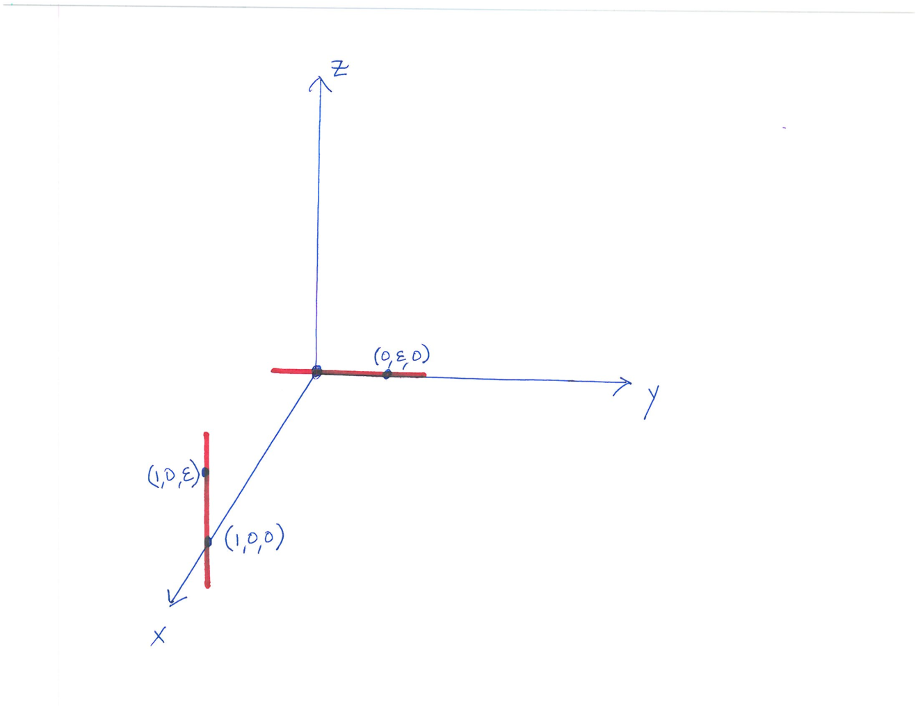
In the applications that we have in mind, we will not able to appeal to Lemma 1.1. However, the distribution $\{V_{y,t}\}$ of $k$-planes in our applications will have an additional regularity property which, as we will see, implies regularity of the set $S$. Roughly speaking, this property is equi-continuity of the distribution $\{V_{y,t}\}$:

Suppose we have a distribution of $k$-dimensional planes $\{V_{y,t}\}$ with $V_{y,t}\subset{\mathbb{R}}^{n+1}\times\{t\}$ labeled by a subset $S\subset{\mathbb{R}}^{n+1}\times{\mathbb{R}}$ with $(y,t)\in V_{y,t}\cap S$. For some $\delta>0$ sufficiently small, let $f:(0,1)\to(0,\delta)$ be a monotone non-decreasing function with $\lim_{r\to 0}f(r)=0$. We will say the distribution $\{V_{y,t}\}$ is $f$-regular if for all $r>0$ and all $(y_{1},t_{1})$, $(y_{2},t_{2})\in S$

for $r={\text{dist}}_{P}((y_{1},t_{1}),(y_{2},t_{2}))$.

Later in our applications to MCF with generic singularities, we will show that not only does the space-time singular set satisfy the strong parabolic (half) vanishing Reifenberg property but the distribution of $k$-planes will be $f$-regular.⁷⁷ 7 In fact, one can take $f(r)\approx(\log|\log r|)^{-\alpha}$ ($\alpha>0$).

The next theorem is the main result of this section. The strong Reifenberg property gives a bi-Lipschitz approximation when the approximating planes are close at nearby points. In Lemma 1.1, (1.2) implies this closeness. If the distribution is $f$-regular, then the closeness is automatic.

The $F$-functional, or Gaussian surface area, of a hypersurface $\Sigma\subset{\mathbb{R}}^{n+1}$ is

where the Gaussian is centered at $x\in{\mathbb{R}}^{n+1}$ and $\sqrt{\tau}>0$ is the scale. The entropy $\lambda$ is the supremum over all Gaussians (i.e., over all centers $x_{0}$ and scales $\sqrt{t_{0}}$)

Huisken’s monotonicity formula⁸⁸ 8 Ilmanen and White extended the monotonicity to the case where $M_{t}$ is a Brakke flow., [H1], for a MCF $M_{t}\subset{\mathbb{R}}^{n+1}$ states that $F_{x,\tau}(M_{t-\tau})$ is increasing in $\tau$ for every fixed $x$ and $t$. That is, if $0<\tau_{1}<\tau_{2}$, then

The monotonicity gives an upper semi-continuous limiting Gaussian density $\Theta_{x,t}$

The limiting density is at least one at each point in the support of the flow and greater than one at each singularity.

By definition, a tangent flow is the limit of a sequence of parabolic dilations at a singularity, where the convergence is on compact subsets. For instance, a tangent flow to $M_{t}$ at the origin in space-time is the limit of a sequence of rescaled flows $\frac{1}{\delta_{i}}\,M_{\delta_{i}^{2}\,t}$ where $\delta_{i}\to 0$. By Huisken’s monotonicity formula and an argument of Ilmanen and White, [I1], [W4], tangent flows are shrinkers, i.e., self-similar solutions of MCF that evolve by rescaling. A priori, different sequences $\delta_{i}$ could give different tangent flows; the question of uniqueness of the blowup is whether the limit is independent of the sequence. In [CM2] (see also [CM5]) it was proven that tangent flows at cylindrical singularities are unique. That is, any other tangent flow is also a cylinder with the same ${\mathbb{R}}^{k}$ factor that points in the same direction.

Throughout this subsection, $M_{t}$ will be a MCF in ${\mathbb{R}}^{n+1}$ with entropy at most $\lambda_{0}$. All constants will be allowed to depend on $n$ and $\lambda_{0}$.

We will let ${\mathcal{C}}_{k}$ denote the cylinder of radius $\sqrt{2(n-k)}$

and its rotations and translations in space.⁹⁹ 9 This is a different convention than in [CM2] where we used $k$ for the dimension of the spherical factor.

It will be useful to have compact notation for spatial rescalings of a set about a fixed point. Namely, given $z\in{\mathbb{R}}^{n+1}$, $r>0$ and $\Lambda\subset{\mathbb{R}}^{n+1}$, let $\Psi_{z,r}(\Lambda)$ be the rescaling of $\Lambda$ about $z$ by the factor $r$, i.e.,

The map $\Psi_{z,r}$ is a rescaling in space only.

We need a notion of what it means for the flow to look like a cylinder near a point. Namely, we will say that $M_{t}$ is $(j,\eta)$-cylindrical at $(y,t)$ on the time-scale $\tau$ if for every positive $s\leq\tau$

• •

  $\Psi_{y,\frac{1}{\sqrt{s}}}\,\left(B_{\eta^{-1}\sqrt{s}}(y)\cap M_{t-s}\right)$ is a graph over a fixed cylinder in ${\mathcal{C}}_{j}$ of a function with $C^{1}$ norm at most $\eta$.

It is important that the dilates $\Psi_{y,\frac{1}{\sqrt{s}}}\,\left(B_{\eta^{-1}\sqrt{s}}(y)\cap M_{t-s}\right)$ are graphs over the same cylinder as the time scale $s$ varies. The constant $j$ here is the dimension of the Euclidean factor of the cylinder. The constant $\eta$ measures how close the flow is to the cylinder in a scale-invariant way and, as $\eta$ gets smaller, the flow is closer to a cylinder on a larger set.

We will need the following result from [CM2] which gives that the flow becomes cylindrical near every cylindrical singularity. Roughly speaking, this says that if the flow is a graph over a cylinder just before a cylindrical singularity, then it remains a graph over the same cylinder as one approaches the singularity. Moreover, after rescaling, it is a graph over a larger set and is even closer to the cylinder.

We will also need a version of $(j,\eta)$-cylindrical where the same time-scale $\tau>0$ works uniformly on a subset $S\subset{\mathcal{S}}$. Namely, $M_{t}$ is uniformly $(j,\eta)$-cylindrical on $S$ on the time-scale $\tau$ if $M_{t}$ is $(j,\eta)$-cylindrical at each $y\in S$ on the time-scale $\tau$. Thus, the axis of the cylinder may vary with $y$, but the time-scale $\tau$ cannot.

In the next corollary, we will fix $j$ and let $S$ be the subset of ${\mathcal{S}}$ with singularity in ${\mathcal{C}}_{j}$.

Given any $y\in{\mathcal{S}}_{j}\setminus{\mathcal{S}}_{j-1}$, the flow is asymptotic to a shrinking cylinder at $y$, i.e., it looks like a cylinder in ${\mathcal{C}}_{j}$ just before $y$. Moreover, by [CM2], this limiting cylinder is unique (it has the same axis on each scale).

The main result of this subsection will show that uniformly $(j,\eta)$-cylindrical subsets of the singular set satisfy a strong Reifenberg property. The dimension of the approximating planes will be the dimension of the affine space for the cylinders.

The following proposition shows that the top strata ${\mathcal{S}}_{n-1}\setminus{\mathcal{S}}_{n-2}$ is always $(n-1,\eta)$-cylindrical on some time-scale $\tau>0$, with a similar statement for the lower strata.

We conclude that ${\mathcal{S}}_{n-1}\setminus{\mathcal{S}}_{n-2}$ has a strong Reifenberg property, with a similar statement for the lower strata:

References

- [AAG] S. Altschuler, S.B. Angenent, and Y. Giga, Mean curvature flow through singularities for surfaces of rotation, Journal of geometric analysis, Volume 5, Number 3, (1995) 293–358.
- [Al] F. J. Almgren, Jr., Q-valued functions minimizing dirichlet’s integral and the regularity of area minimizing rectiable currents up to codimension two, preprint.
- [An] B. Andrews, Noncollapsing in mean-convex mean curvature flow. Geom. Topol. 16 (2012), no. 3, 1413–1418.
- [Ba] R. Bamler, Long-time behavior of 3 dimensional Ricci flow – Introduction, preprint.
- [BeWa] J. Bernstein and L. Wang, A Remark on a Uniqueness Property of High Multiplicity Tangent Flows in Dimension Three, preprint, http://arxiv.org/abs/1402.6687.
- [B] K. Brakke, The motion of a surface by its mean curvature. Mathematical Notes, 20. Princeton University Press, Princeton, N.J., 1978.
- [ChCT] J. Cheeger, T.H. Colding, and G. Tian, Constraints on singularities under Ricci curvature bounds. C. R. Acad. Sci. Paris Sér. I Math. 324 (1997), no. 6, 645–649.
- [CGG] Y. G. Chen, Y. Giga, and S. Goto, Uniqueness and existence of viscosity solutions of generalized mean curvature flow equations, J. Diff. Geom., 33 (1991), 749–786.
- [CIM] T.H. Colding, T. Ilmanen and W.P. Minicozzi II, Rigidity of generic singularities of mean curvature flow, Public. IHES, DOI 10.1007/s10240-015-0071-3, arXiv:1304.6356.
- [CK] T.H. Colding and B. Kleiner, Singularity structure in mean curvature flow of mean-convex sets. Electron. Res. Announc. Amer. Math. Soc. 9 (2003), 121–124.
- [CM1] T.H. Colding and W.P. Minicozzi II, Generic mean curvature flow I; generic singularities, Annals of Math., 175 (2012), Issue 2, 755–833.
- [CM2] by same author, Uniqueness of blowups and Łojasiewicz inequalities, Annals of Math., to appear, arXiv:1312.4046.
- [CM3] by same author, The space of embedded minimal surfaces of fixed genus in a 3-manifold. IV. Locally simply connected. Annals of Math. (2) 160 (2004), no. 2, 573–615.
- [CM4] by same author, The space of embedded minimal surfaces of fixed genus in a 3-manifold. V. Finite genus, Annals of Math., 181 (2015), 1–153.
- [CM5] by same author, Łojasiewicz inequalities and applications, Surveys in Differential Geometry XIX, International Press, to appear, arXiv:1402.5087.
- [CM6] by same author, Differentiability of the arrival time, preprint, arXiv:1501.07899.
- [CMP] T.H. Colding, W.P. Minicozzi II and E.K. Pedersen, Mean curvature flow, Bulletin of the AMS, 52 (2015), no. 2, 297–333.
- [DKT] G. David, C. Kenig, and T. Toro, Asymptotically optimally doubling measures and Reifenberg flat sets with vanishing constant, Comm. Pure Appl. Math. 54 (2001), no. 4, 385–449.
- [D] C. De Lellis, Rectifiable sets, densities and tangent measures. Zurich Lectures in Advanced Mathematics. European Mathematical Society (EMS), Zürich, 2008.
- [E] K. Ecker, Regularity theory for mean curvature flow. Progress in Nonlinear Differential Equations and their Applications, 57. Birkhäuser Boston, Inc., Boston, MA, 2004.
- [ES] L. C. Evans and J. Spruck, Motion of level sets by mean curvature I, J. Diff. Geom., 33 (1991), no. 3, 635–681; II, Trans. Amer. Math. Soc., 330 (1992), no. 1, 321–332; III, J. Geom. Anal., 2 (1992), no. 2, 121–150; IV, J. Geom. Anal., 5 (1995), no. 1, 77–114.
- [F1] H. Federer, Geometric measure theory. Die Grundlehren der mathematischen Wissenschaften, Band 153 Springer-Verlag New York Inc., New York 1969.
- [F2] by same author, The singular sets of area minimizing rectifiable currents with codimension one and of area minimizing flat chains modulo two with arbitrary codimension. Bull. Amer. Math. Soc. 76 (1970) 767–771.
- [HaK] R. Haslhofer and B. Kleiner, Mean curvature flow of mean convex hypersurfaces, preprint, http://arXiv:1304.0926.
- [HoW] G. Hong and L. Wang, A geometric approach to the topological disk theorem of Reifenberg, Pacific J. Math. 233 (2007), no. 2, 321–339.
- [H1] G. Huisken, Asymptotic behavior for singularities of the mean curvature flow. J. Differential Geom. 31 (1990), no. 1, 285–299.
- [H2] by same author, Local and global behaviour of hypersurfaces moving by mean curvature. Differential geometry: partial differential equations on manifolds (Los Angeles, CA, 1990), 175–191, Proc. Sympos. Pure Math., 54, Part 1, Amer. Math. Soc., Providence, RI, 1993.
- [HS1] G. Huisken and C. Sinestrari, Convexity estimates for mean curvature flow and singularities of mean convex surfaces, Acta Math. 183 (1999) no. 1, 45–70.
- [HS2] by same author, Mean curvature flow singularities for mean convex surfaces, Calc. Var. Partial Differ. Equ. 8 (1999), 1–14.
- [HS3] by same author, Mean curvature flow with surgeries of two-convex hypersurfaces. Invent. Math. 175 (2009), no. 1, 137–221.
- [I1]
T. Ilmanen,
Singularities of Mean Curvature Flow of Surfaces, preprint, 1995,
http://www.math.ethz.ch/˜/papers/pub.html. - [I2] by same author, Elliptic regularization and partial regularity for motion by mean curvature, Memoirs Amer. Math. Soc. 520 (1994).
- [LjT] J. Li and G. Tian, The blow-up locus of heat flows for harmonic maps. Acta Math. Sin. (Engl. Ser.) 16 (2000), no. 1, 29–62.
- [LW] F.-H. Lin and C.-Y. Wang, Harmonic and quasi-harmonic spheres. III. Rectifiability of the parabolic defect measure and generalized varifold flows. Ann. Inst. H. Poincar� Anal. Non Lin�aire 19 (2002), no. 2, 209–259.
- [LY] F.-H. Lin and X. Yang, Geometric measure theory – an introduction. Advanced Mathematics (Beijing/Boston), 1. Science Press Beijing, Beijing; International Press, Boston, MA, 2002.
- [OS] S. Osher and J. Sethian, Fronts propagating with curvature-dependent speed: algorithms based on Hamilton-Jacobi formulations, J. Comput. Phys., 79 (1988), 12–49.
- [P] D. Preiss, Geometry of measures in : distribution, rectifiability, and densities. Ann. of Math. (2) 125 (1987), no. 3, 537–643.
- [PTT] D. Preiss, X. Tolsa and T. Toro, On the smoothness of Hölder-doubling measures, Calculus of Variations and PDE 35 (2009), 339–363.
- [R] E.R. Reifenberg, Solution of the Plateau Problem for m-dimensional surfaces of varying topological type. Acta Math. 104 (1960), 1–92.
- [S1] L. Simon, Rectifiability of the Singular Sets of Multiplicity 1 Minimal Surfaces and Energy Minimizing Maps, Surveys in Diff. Geom. 2 (1995), 246–305.
- [S2] by same author, Rectifiability of the singular set of energy minimizing maps, Cal. of Var. and PDE’s, (1995), Volume 3, Issue 1, 1–65.
- [SrSs] H. Soner and P. Souganidis, Singularities and uniqueness of cylindrically symmetric surfaces moving by mean curvature. Comm. Partial Differential Equations 18 (1993), no. 5-6, 859–894.
- [T] T. Toro, Doubling and Flatness: Geometry of Measures, Notices of the AMS, 44, 1997, 1087–1094.
- [W1] B. White, The nature of singularities in mean curvature flow of mean-convex sets. J. Amer. Math. Soc. 16 (2003), no. 1, 123–138.
- [W2] by same author, The size of the singular set in mean curvature flow of mean-convex sets, J. Amer. Math. Soc. 13 (2000), 665–695.
- [W3] by same author, Evolution of curves and surfaces by mean curvature. Proceedings of the International Congress of Mathematicians, Vol. I (Beijing, 2002), 525–538.
- [W4] by same author, Partial regularity of mean-convex hypersurfaces flowing by mean curvature, Int. Math. Res. Notices (1994) 185–192.
- [W5] by same author, Stratification of minimal surfaces, mean curvature flows, and harmonic maps, J. Reine Angew. Math. 488 (1997), 1–35.
- [W6] by same author, Subsequent singularities in mean-convex mean curvature flow, arXiv:1103.1469, 2011.