Majorana Braiding Dynamics on Nanowires

Introduction— Recent discovery of topological matters provides a novel platform of quantum devices. In particular , topological superconductors naturally realize yet-to-be discovered excitations called Majorana fermions as a collective mode in condensed matter physics [1, 2, 3]. Because of the self-antiparticle nature, the isolated Majorana zero modes display unusual physical properties such as non-Abelian anyon statistics, which is of extreme interest in realization of topological quantum computer in reality.

Topological superconductivity was originally recognized in $p$-wave spin-triplet superconductors [4, 5, 6, 7], however, advance on our understanding of topological matters enables us to design it even in a conventional $s$-wave superconducting state [8, 9, 10, 11]. A recent proposed scheme to realize Majorana fermions by using the spin-orbit interaction and Zeeman field [12, 10, 13, 11, 14] was eventually applied to a one-dimensional nanowire with proximity induced $s$-wave pairing [15, 16], which can be fabricated by the present experimental technique [17, 18, 19, 20, 21, 22]. Furthermore, varieties of proposals exist in order to improve the experimental accessibility and controllability of Majorana modes [23, 24, 25, 26, 27, 28, 29, 30, 31, 32, 33, 34, 35].

In topological quantum computation, quantum operations of qubits are implemented as an exchange process of Majorana zero modes. Thus, a crucial next step toward topological quantum computer is to understand such an operation of collective excitations as a time-dependent dynamical process.

In this paper, we investigate the braiding dynamics of Majorana zero modes on superconducting nanowires. Generalizing proposed methods of Majorana braiding [36, 37, 38, 39, 40, 41, 42, 43, 44, 45, 46, 47, 48, 49, 50], we consider a simpler cruciform junction of topologically non-trivial superconducting nanowires. This simple system functions as a quantum NOT gate of a Majorana qubit by switching gates connecting the wires to the cross point. Using this model, we simulate the Majorana braiding by solving the time-dependent Bogoliubov de Genne equation for the nanowires. A non-adiabatic dynamical process dominates the non-Abelian braiding that operates qubits of Majorana fermions. Our simulations clarify how qubits behave in the real-time braiding process, and elucidate the optimum condition of superconducting nanowires for efficient topological quantum operation.

Majorana Braiding— In the low energy limit, one-dimensional topological superconductors reduce to a one-dimensional spinless $p_{x}$-wave superconductor. We adopt the spinless $p_{x}$-wave superconductor as a model to analyze universal aspects of Majorana dynamics on nanowires,

where $c_{x}$ is a spinless fermion operator and $\mu$, $\lambda$ and $\Delta e^{i\theta}$ are the chemical potential, the hopping integral, and the $p$-wave pairing potential, respectively. ($\lambda>0$, $\Delta>0$.) There are two different topological phases in the spinless $p_{x}$-wave superconductor [6]. When $|\mu|<\lambda$, the $p_{x}$-wave superconductor realizes a topologically non-trivial superconducting state, and thus it supports a Majorana fermion on each end. In contrast, when $|\mu|>\lambda$, it becomes a topologically trivial state without Majorana end modes. Below, we consider $p_{x}$-wave superconducting nanowires in the topologically non-trivial phase.

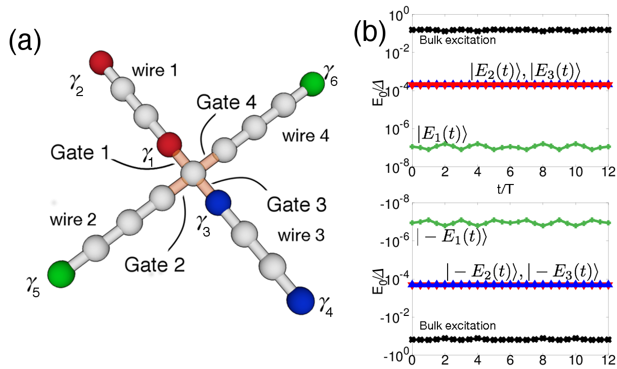
To braid the Majorana end states, we consider a cruciform junction illustrated in Fig.1 (a), where four topologically non-trivial nanowires (wire 1, 2, 3 and 4) are connected by four gates (gate 1, 2, 3 and 4). The hopping integral $\lambda$ and the paring potential $\Delta$ at the gates are tunable, so one can connect (disconnect) the wires by turning on (off) these parameters at the gates.

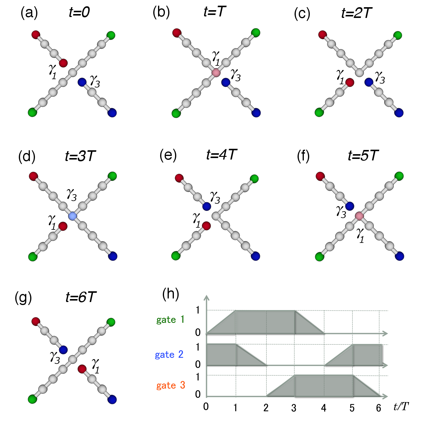
Now let us illustrate how one can exchange the Majorana end modes by switching these gates of the cruciform junction. Initially, we prepare the configuration of Fig.2(a), where wires 2 and 4 are connected by turning on gates 2 and 4, while wires 1 and 3 are disconnected. There are six Majorana end states in the initial configuration since two Majorna end states at the inner edge of wires 2 and 4 are gapped by the coupling at gates 2 and 4.

Counterclockwise exchange of the Majorana modes $\gamma_{1}$ and $\gamma_{3}$, which are localized at the inner edges of wires 1 and 3, can be implemented as follows: First, by turning on the gate 1 [Fig. 2(b)] and then turning off gate 2 [Fig. 2(c)], $\gamma_{1}$ moves to the inner edge of wire 2. Next, $\gamma_{3}$ moves to the inner edge of wire 1 by turning on gate 3 [Fig. 2(d)] and then turning off gate 1 [Fig. 2(e)]. Finally, $\gamma_{1}$ moves to the inner edge of wire 3 by turning on gate 2 [Fig. 2(f)] and then turning off gate 3 [Fig. 2(g)]. The final gate configuration is identical to the initial one, but $\gamma_{1}$ and $\gamma_{3}$ are exchanged.

In the initial configuration $(t=0)$, wire 1 and wire 3 are isolated from others. While wires 2 and 4 are connected to each other, they are also disconnected from the rest. Due to the finite length of wires, the mixing of Majorana modes occurs between $\gamma_{1}$ and $\gamma_{2}$, $\gamma_{3}$ and $\gamma_{4}$, and $\gamma_{5}$ and $\gamma_{6}$, respectively [6, 51, 52, 53, 54]. It induces the following effective coupling between zero modes,

where the constants $\epsilon$ and $\epsilon^{\prime}$ are real because ${\cal H}$ should be hermitian, and $\epsilon$ is larger than $\epsilon^{\prime}$ since the coupling between $\gamma_{5}$ and $\gamma_{6}$ is weaker than the others. Assuming the standard anti-commutation relation of Majorana zero modes, i.e. $\{\gamma_{i},\gamma_{j}\}=2\delta_{ij}$, ${\cal H}$ can be recast into

with the Dirac operators

obeying $\{c_{i},c_{j}^{\dagger}\}=\delta_{ij}$. Therefore, the mixing results in three negative energy states $|-E_{i}\rangle$ $(i=1,2,3)$ that are annihilated by $c_{i}$,

and three positve partners $|E_{i}\rangle$ that are annihilated by $c_{i}^{\dagger}$,

with $E_{1}=\epsilon^{\prime}$ and $E_{2}=E_{3}=\epsilon$.

By switching the gates as described above, we can exchange the Majorana zero modes $\gamma_{1}$ and $\gamma_{3}$. A proper gating process for the non-Abelian braiding does not merely interchange $\gamma_{1}$ and $\gamma_{3}$, but also provide a non-trivial relative phase between them, $\gamma_{1}\rightarrow-\gamma_{3}$, $\gamma_{3}\rightarrow\gamma_{1},$ or $\gamma_{1}\rightarrow\gamma_{3}$, $\gamma_{3}\rightarrow-\gamma_{1}$. In both cases, if we exchange $\gamma_{1}$ and $\gamma_{3}$ twice, $\gamma_{1}$ and $\gamma_{3}$ do not go back to the original, but they acquire the minus sign, $\gamma_{1}\rightarrow-\gamma_{1},$ $\gamma_{3}\rightarrow-\gamma_{3}.$ Therefore, after exchange $\gamma_{1}$ and $\gamma_{3}$ twice, the Dirac operators $c_{2}$ and $c_{3}$ transform into their conjugates $-c_{2}^{\dagger}$ and $-c_{3}^{\dagger}$ as

The nontrivial transformation of $c_{2}$ and $c_{3}$ implies that the negative energy states $|-E_{2}\rangle$ and $|-E_{3}\rangle$, which are annihilated by $c_{2}$ and $c_{3}$, respectively, end up as the positive energy partners $|E_{2}\rangle$ and $|E_{3}\rangle$, and vice versa, after the exchange process. In other words, if we choose these negative energy states as an initial state, the final state is orthogonal to the initial one. This complete interference is a direct signal of the non-Abelian anyon statistics: Indeed if the system obeys an ordinary Abelian statistics, any exchange process results in a phase factor for any initial state, so the final state cannot be orthogonal to the initial one. The above exchange process defines a quantum NOT gate for Majorana qubits $(|E_{2}\rangle,|-E_{2}\rangle)$ and $(|E_{3}\rangle,|-E_{3}\rangle)$.

Whereas the above procedure eventually works well as is shown below, the actual implementation needs a careful consideration for the gating. In Fig.1 (b), we show lower energy eigenvalues of the system as a function of $t$. The eigen energies $E_{1}(t)$, $E_{2}(t)$, $E_{3}(t)$ and their negative energy partners correspond to six Majorana zero modes of the system, where $E_{2}(t)$ and $E_{3}(t)$ are degenerate within numerical accuracy as well as their negative energy partners are. At $t=0$, these eigen energies coincide with $E_{i}$ $(i=1,2,3)$ in the above, $E_{i}(0)=E_{i},$ and we also have $E_{i}(6T)=E_{i}(12T)=E_{i}$ since the system goes back to the initial configuration at $t=6T$ and $12T$. We note here that there is no level crossing in the energy spectrum in Fig.1 (b), as expected from the von Neumann-Wigner theorem [55]. Therefore, a non-adiabatic transition is needed to achieve the non-Abelian braiding discussed in the above, since any state cannot be different from the original under an adiabatic process. Namely, the gating process in Fig.2 should not be too slow. The non-adiabatic transition is not a classical Landau-Zener transition, because the level spacing rarely depends on $t$ and there is no level approaching to each other at a particular time. We can also argue that a proper gating process should not be too fast at the same time. A fast gating process may create bulk excitations on nanowires, which may give rise to problematic decoherence of Majorana qubits. Therefore, the gating process for non-Abelian braiding should be performed at a proper range of speed.

Below we operate the gates 1, 2, 3 in accordance with the time-sequence diagram in Fig.2 (h). The gating speed can be controlled by an adiabatic parameter $T$: The gate operation becomes slower (faster) and more adiabatic (non-adiabatic) for larger (smaller) $T$. A moderate $T$ is required to realize the non-Abelian braiding.

Braiding Dynamics— We now numerically simulate the Majorana braiding process in Fig.2. To numerically evaluate our system, we take each wire length to be the same with one central site linking them. Each gate is represented as a factor $g_{i}\in[0,1]$ ($i=1,2,3,4$) multiplying the link on the gates in real space ¹¹ 1 For details, see Supplementary Material.. The dynamics of the system is described by the time-dependent Bogoliubov-de Genne equation

where $\Psi(t)$ is the quasiparticle wavefunction in the Nambu representation. The evaluation of the wavefunction during a time ${\mathit{\Delta}}t$ is given by $\Psi(t+{\mathit{\Delta}}t)={\cal U}(t+\mathit{\Delta}t;t)\Psi(t)$ with the time-evolution operator ${\cal U}(t+{\mathit{\Delta}}t;t)$,

which is well-approximated as ${\cal U}(t+\mathit{\Delta}t,t)\approx\exp\left[-i{\cal H}(t)\mathit{\Delta}t\right]$, within numerical errors for a sufficiently short $\mathit{\Delta}t$. To achieve a correct wavefunction change in time, we further expand the time-evolution operator in terms of Chebishev polynomials [56, 38], which can be retrieved recursively, that is

where $E_{0}\equiv\max|\langle\Psi|\mathcal{H}|\Psi\rangle|$ normalizes the Hamiltonian to avoid singularities of Chebishev polynomials and

constitute our expansion terms. Here $\tilde{H}={\cal H}/E_{0}$, $\mathit{\Delta}\tau=\mathit{\Delta}tE_{0}$, and $J_{k}$ are the Bessel functions of first kind. For small $\mathit{\Delta}\tau$, the coefficients $c_{k}(\mathit{\Delta}\tau)$ rapidly converge to zero as $k$ increases. Thus keeping the first few expansion terms in the right hand side of Eq.(10) is enough to reach numerically reliable results.

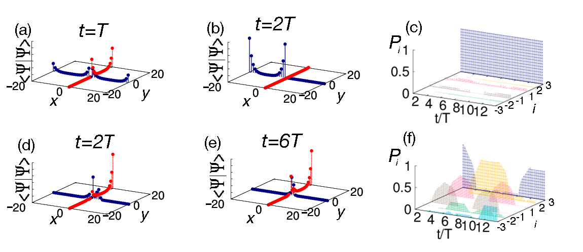
Figure 3 is one of the main results in this paper. In Fig.3, we illustrate how the wavefunction evolves in time in our numerical simulation of the non-Abelian braiding. We choose $|E_{3}\rangle$ as the initial state at $t=0$, and take $T=100/\Delta$. It demonstrates that only the inner part of the wave function moves in time, which exactly corresponds to the movement of Majorana mode $\gamma_{1}$. At $t=6T$, although the gate configuration goes back to the initial one, the inner part of the wave function moves to the inner edge of wire 3, which indicates that $\gamma_{1}$ is successfully interchanged with $\gamma_{3}$. Then finally, the inner part goes back to the initial position at $t=t_{\rm f}\equiv 12T$.

We project the same wavefunction into the instantaneous eigenstates $|\pm E_{i}(t)\rangle$ $(i=1,2,3)$ in Fig.3 (f). Initially, the wavefunction consists of only $|E_{3}\rangle$, but after the gating process starts, the wave function quickly spreads over the eigenstates $|-E_{3}\rangle$ and $|\pm E_{3}\rangle$. Nevertheless, the final state ends up at $|-E_{3}\rangle$, as expected as the non-Abelian braiding process mentioned above.

If one operates the gates too slowly or too quickly, the non-Abelian braiding fails. For example, in the slow gating with $T=100000/\Delta$, both inner and outer Majorana modes of wire 1 move together in time, in which the state mostly stays at the instantaneous eigenstate $|E_{3}(t)\rangle$, as expected by the adiabatic theorem. On the other hand, for the quick gating with $T=1/\Delta$, the wave function extends over all eigenstates $|\pm E_{i}(t)\rangle$ $(i=1,2,3)$, and it never goes back to the initial state. In the latter case, the wave function in the final state also spreads over nanowires in space, which suggests that bulk modes are excited during the gating. We exemplify these unsuccessful braiding in Fig. 4.

To quantify the non-Abelian braiding, we introduce its success rate $P_{\rm s}$ as the probability that the final state $|\Psi(t_{\rm f})\rangle$ is found to be the desired state $|-E_{3}\rangle$,

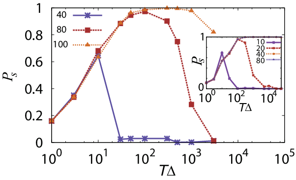
In Fig.5, we plot the success rate $P_{\rm s}$ versus the adiabatic parameter $T$, with various wire lengths. The data indicates that a longer wire is desirable for the non-Abelian braiding. For longer wires, the success rate can reach the maximum, i.e. $P_{\rm s}=1$ for large $T$. In a shorter wire, on the other hand, a Majorana end mode is fairly coupled with the Majorana mode on the other end, so they tend to move together, resulting in an adiabatic process even for a moderate $T$. We also find that a quicker gating fails to achieve the non-Abelian braiding for any length of wires, since it excites undesirable bulk modes.

Finally, from our numerical results, we evaluate the optimal condition for non-Abelian braiding. We note that $T$ should be larger than the inverse of the bulk gap $1/\Delta$, not to excite bulk modes. Our numerical data determines how large it should be. Figure 5 indicates that the lower bound $T$ is not a merely $O(1/\Delta)$, but it is evaluated as $T_{\rm min}\sim O(10^{2}/\Delta)$. For a typical superconducting state with $\Delta=O(1)$ K, $T_{\rm min}$ can be a few nanoseconds. On the other hand, the upper bound of $T$ can be determined as follows. As we illustrated in the above, the non-Abelian braiding is realized as an non-adiabatic process between Majorana modes. Thus, for Majorana modes with energy $\epsilon$, $\epsilon T$ should not be too large. Our numerical results imply that the success rate of the non-Abelian braiding $P_{\rm s}$ reaches almost the maximum when $\epsilon T$ is less than $O(10)$. The latter condition can be easily met for long wires, since $\epsilon$ scales as $\epsilon\sim e^{-N/l_{0}}$. It is also found in Fig. 5 that the quantum limit of superconducting state, i.e. $\Delta/\lambda=1$, requires less numbers of sites for the non-Abelian braiding, which is preferable if one realizes topological supercondicting wires as a chain of quantum dots.[33]

The authors are grateful to J. D. Sau and K. T. Law for fruitful discussions. This work was supported by the JSPS (No.25287085) and KAKENHI Grants-in-Aid (No.22103005) from MEXT. C.S.A. is supported by MEXT Scholarship (kokuhi-gaikokujin-ryugakusei 2013)

Supplementary Material

References

- [1] Y. Tanaka, M. Sato, and N. Nagaosa, J. Phys. Soc. Jpn. 81, 011013 (2012).
- [2] X. L. Qi and S. C. Zhang, Rev. Mod. Phys. 83, 1057 (2011).
- [3] F. Wilczek, Nat. Phys. 5, 614 (2009).
- [4] N. Read and D. Green, Phys. Rev. B 61, 10267 (2000).
- [5] D. A. Ivanov, Phys. Rev. Lett. 86, 268 (2001).
- [6] A. Y. Kitaev, Physics-Uspekhi 44, 131 (2001).
- [7] M. Sato, Phys. Rev. B 81, 220504(R) (2010).
- [8] M. Sato, Phys. Lett. B 575, 126 (2003).
- [9] L. Fu and C. L. Kane, Phys. Rev. Lett. 100, 096407 (2008).
- [10] M. Sato, Y. Takahashi, and S. Fujimoto, Phys. Rev. Lett. 103, 020401 (2009).
- [11] J. D. Sau, R. M. Lutchyn, S. Tewari, and S. D. Sarma, Phys. Rev. Lett. 104, 040502 (2010a).
- [12] M. Sato and S. Fujimoto, Phys. Rev. B 79, 094504 (2009).
- [13] M. Sato, Y. Takahashi, and S. Fujimoto, Phys. Rev. B 82, 134521 (2010).
- [14] J. Alicea, Phys. Rev. B 81, 125318 (2010).
- [15] R. M. Lutchyn, J. D. Sau, and S. D. Sarma, Phys. Rev. Lett. 105, 077001 (2010).
- [16] Y. Oreg, G. Refael, and F. von Oppen, Phys. Rev. Lett. 105, 177002 (2010).
- [17] V. Mourik, K. Zuo, S. Frolov, S. Plissard, E. Bakkers, and L. Kouwenhoven, Science 336, 1003 (2012).
- [18] M. Deng, C. Yu, G. Huang, M. Larsson, P. Caro, and H. Xu, Nano Lett. 12, 6414 (2012).
- [19] A. Das, Y. Ronen, Y. Most, Y. Oreg, M. Heiblum, and H. Shtrikman, Nat. Phys. 8, 887 (2012).
- [20] J. Williams, A. Bestwick, P. Gallagher, S. Hong, Y. Cui, A. Bleich, J. Analytis, I. Fisher, and D. Goldhaber-Gordon, Phys. Rev. Lett. 109, 056803 (2012).
- [21] M. Veldhorst, M. Snelder, M. hoek, T. Gang, V. Guduru, X. L. Wang, U. Zeitler, W. G. van der Wiel, A. A. Golubov, H. Hilgenkamp, et al., Nat. Mater. 11, 417 (2012).
- [22] L. P. Rokhinson, X. Liu, and J. K. Furdyna, Nat. Phys. 8, 795 (2012).
- [23] J. Linder, Y. Tanaka, T. Yokoyama, A. Sudbo, and N. Nagaosa, Phys. Rev. Lett. 104, 067001 (2010).
- [24] M. Sato and S. Fujimoto, Phys. Rev. Lett. 105, 217001 (2010).
- [25] J. Alicea, Rep. Prog. Phys. 75, 076501 (2012).
- [26] T. D. Stanescu and S. Tewari, J. Phys.: Condens. Matter 25, 233201 (2013).
- [27] C. W. J. Beenakker, Annu. Rev. Con. Mat. Phys. 4, 113 (2013).
- [28] F. Hassler, Quantum Information Processing. Lecture notes of the 44th IFF Spring School 2013 (2013).
- [29] J. D. Sau, S. Tewari, R. M. Lutchyn, T. D. Stanescu, and S. D. Sarma, Phys. Rev. B 82, 214509 (2010b).
- [30] J. Klinovaja and D. Loss, Phys. Rev. B 86, 085408 (2012).
- [31] J. D. Sau, C. H. Lin, H.-Y. Hui, and S. D. Sarma, Phys. Rev. Lett. 108, 067001 (2012).
- [32] D. Chevallier, D. Sticlet, P. Simon, and C. Bena, Phys. Rev. B 87, 165414 (2013).
- [33] J. D. Sau and S. D. Sarma, Nat. Comm. 3, 964 (2012).
- [34] S. Nakosai, J. C. Budich, Y. Tanaka, B. Trauzettel, and N. Nagaosa, Phys. Rev. Lett. 110, 117002 (2013).
- [35] S. Mi, D. I. Pikulin, M. Wimmer, and C. W. J. Beenakker, Phys. Rev. B 87, 241405 (2013).
- [36] J. Alicea, Y. Oreg, G. Refael, F. von Oppen, and M. P. A. Fisher, Nat. Phys. 7, 412 (2011).
- [37] J. Sau, D. Clarke, and S. Tewari, Phys. Rev. B 84, 094505 (2011).
- [38] Q. Liang, Z. Wang, and X. Hu, Euro Physics Letters 99, 50004 (2012).
- [39] P. Kotetes, G. Schön, and A. Shnirman, Journal of the Korean Physical Society 62, 1558 (2013).
- [40] B. I. Halperin, Y. Oreg, A. Stern, G. Refael, J. Alicea, and F. von Oppen, Phys. Rev. B 85, 144501 (2012).
- [41] J. D. Sau, S. Tewari, and S. D. Sarma, Phys. Rev. A 82, 052322 (2010c).
- [42] X. J. Liu, C. L. M. Wong, and K. T. Law, eprint arXiv:1304.3765.
- [43] F. Zhang, C. L. Kane, and E. J. Mele, Phys. Rev. Lett. 111, 056403 (2013).
- [44] J. Li, T. Neupert, B. A. Bernevig, and A. Yazdani, eprint arXiv:1404.4058.
- [45] L. Weithifer, P. Recher, and T. L. Schimidt, eprint arXiv:1309.4126.
- [46] T. Karzig, G. Refael, and F. von Oppen, Phys. Rev. X 3, 041017 (2013).
- [47] T. Hyart, B. van Heck, I. C. Fulga, M. Burrello, A. R. Akhmerov, and C. W. J. Beenakker, Phys. Rev. B 88, 035121 (2013).
- [48] C. V. Kraus, P. Zoller, and M. A. Baranov, Phys. Rev. Lett. 111, 203001 (2013).
- [49] X.-J. Liu and A. M. Lobos, Phys. Rev. B 87, 060504 (2013).
- [50] C.-K. Chiu, M. Vazifeh, and M. Franz, eprint arXiv:1403.0033v1.
- [51] M. Cheng, R. M. Lutchyn, V. Galitski, and S. D. Sarma, Phys. Rev. Lett. 103, 107001 (2009).
- [52] T. Mizushima and K. Machida, Phys. Rev. A 82, 023624 (2010).
- [53] M. Cheng, R. M. Lutchyn, V. Galitski, and S. D. Sarma, Phys. Rev. B 82, 094504 (2010).
- [54] M. Cheng, V. Galitski, and S. D. Sarma, Phys. Rev. B 84, 104529 (2011).
- [55] J. von Neumann and E. P. Wigner, Z. Phys. 30, 467 (1929).
- [56] H. Tal-Ezer and R. Kosloff, Jour. Chem. Phys. 81 (1984).
- [57] D. Göddeke, R. Strzodka, and S. Turek, International Journal of Parallel, Emergent and Distributed Systems (IJPEDS), Special issue: Applied parallel computing 22, 221 (2007).
- [58] M. Baboulin, A. Buttari, J. Dongarra, J. Kurzak, J. Langou, J. Langou, P. Luszczek, and S. Tomov, Comp. Phys. Comm. 180, 2526 (2009).
- [59] S. L. Grand, A. W. Götz, and R. C. Walker, Comp. Phys. Comm. 184, 374 (2013).