CHARACTERIZING THE CONVECTIVE VELOCITY FIELDS IN MASSIVE STARSNote: Submitted to ApJ on 2014 May 17
Abstract
We apply the mathematical formalism of vector spherical harmonics decomposition to convective stellar velocity fields from multi-dimensional hydrodynamics simulations, and show that the resulting power spectra furnish a robust and stable statistical description of stellar convective turbulence. Analysis of the power spectra help identify key physical parameters of the convective process such as the dominant scale of the turbulent motions that influence the structure of massive evolved pre-supernova stars. We introduce the numerical method that can be used to calculate vector spherical harmonics power spectra from 2D and 3D convective shell simulation data. Using this method we study the properties of oxygen shell burning and convection for a 15- star simulated by the hydrodynamics code FLASH in 2D and 3D. We discuss the importance of realistic initial conditions to achieving successful core-collapse supernova explosions in multi-dimensional simulations. We show that the calculated power spectra can be used to generate realizations of the velocity fields of pre-supernova convective shells. We find that the slope of the solenoidal mode power spectrum remains mostly constant throughout the evolution of convection in the oxygen shell in both 2D and 3D simulations. We also find that the characteristic radial scales of the convective elements are smaller in 3D than in 2D while the angular scales are larger in 3D.
Subject headings
methods: numerical — stars: convection — stars: massive — supernovae: general, supernovae: individual (progenitors)I. INTRODUCTION
Many astrophysical systems are characterized by highly anisotropic, turbulent or even chaotic motions of their constituents. The case of energy transport in stellar interiors via convection is a classic example. Depending on a star’s mass and age convective instability can be triggered by nuclear burning and may arise in several parts of the stellar interior (core or shell convection).
Due to computational limitations the effects of convection on stellar evolution have predominantly been studied via the use of one-dimensional spherically symmetric stellar evolution codes such as KEPLER [37, 38], TYCHO [39] the GENEVA code [10] and more recently the Modules for Experiments in Stellar Astrophysics (MESA) [24, 25]. All of these codes use the standard mixing-length theory (MLT) to treat convection based on either the Schwarzschild or the Ledoux criteria plus parametrized treatments for the effects of semi-convection, convective overshoot and thermohaline mixing (see, e.g., Heger et al. [13]). A topic of current debate is how accurate those parametrized MLT prescriptions are as compared to intrinsically three-dimensional simulations of convection.
Significant efforts have been made to simulate stellar convection in multiple dimensions over a timescale short compared to the evolutionary timescale, and to compare the output of such simulations to the parametrized predictions. [21] presented multi-dimensional simulations of oxygen shell burning and hydrogen core burning for a 23- core-collapse supernova (CCSN) progenitor star. They found significant differences between the 2D and the 3D treatment and underscored the fact that the convective mixing regions are better predicted using dynamic boundary conditions (BCs) rather than local and static MLT criteria. This dynamical behavior of convective boundaries is found to be a source of gravity waves that can, under certain circumstances, lead to episodic mass-loss in the years preceding the supernova (SN) explosion [27, 28]. Such pre-SN mass loss events can give rise to supernova impostors, as is the case with the pre-explosion outbursts of SN 2009ip [17, 16, 30]. Similar studies have been done in the case of main-sequence (MS) core convection [12] and vigorous pre-SN convection (with emphasis on energetic Si-shell burning) in the hours prior to core collapse [19, 3], also Couch et al. (2014, in preparation).
These multi-dimensional studies exhibit pronounced shell asymmetries and dynamical interactions between adjacent convective regions. Such effects can significantly change the structure not only of the pre-SN star but of its circumstellar (CS) environment [23], and, as a result, can affect the initial conditions for the core-collapse process and subsequent explosion. Indeed, it has recently been shown that the outcome of CCSN simulations can be qualitatively different for realistic aspherical initial conditions. [6] show that imprinting physically-motivated velocity fluctuations in the convective regions of the progenitor star prior to collapse can result in shock revival in 3D CCSN simulations that fail to explode otherwise.
The importance of initializing such velocity perturbations in order to characterize the multi-dimensional nature of pre-SN convection has been pointed out in the past and several formalisms have been proposed, including scalar spherical harmonics and Fourier decomposition [5] that are commensurate with the Kolmogorov energy spectrum expected for highly turbulent stellar regions. Fourier modes, however, are poor matches to the spherical boundary conditions relevant to this problem. In addition, other approaches such as the spherical Fourier-Bessel decomposition have attempted to analyze scalar fields in CCSN convection Fernández et al. [11] in spherical, concentric shells. In this paper we introduce a mathematical framework for analyzing stochastic stellar velocity fields, the method of decomposition into vector spherical harmonics (VSH), and apply the method to the case of CCSN progenitor convection. VSH decomposition of multi-dimensional simulation data can be used to extract power spectra that describe the distribution of convective power over the length scales of the system. VSH power spectra can also be used to produce realizations of velocity fields that capture the non-radial perturbations of the flow due to convection, and therefore provide more realistic initial conditions for multi-dimensional CCSN simulations. The toolset of VSH has been used in other fields of astrophysics where random velocity distributions are present such as the local stellar velocity field [22] and stellar pulsations and oscillations [29, 15].
Our paper is organized as follows: in Section II we present the basic mathematical formulation of VSH, in Section III we discuss the numerical evaluation of VSH and relevant consistency tests that illustrate the accuracy of our results and apply the method to the case of a 2D oxygen shell burning simulation. In Section IV we apply VSH decomposition to a 3D oxygen shell burning simulation and discuss the differences between the corresponding power spectra. Finally, in Section V we summarize our conclusions and discuss the importance of this technique to setting realistic initial conditions for the CCSN simulations.
II. THE FORMULATION OF VSH
Much of the VSH formulation described below is based on material in Morse & Feshbach [18], Chandrasekhar [4], Jackson [14] and Arfken & Weber [1]. Details on the derivation of the VSH modes, their orthonormality relations, proper treatment of boundary conditions as well as dependence on data dimensionality and simulation domain can be found in Appendix A.
We seek to characterize velocity fields that we may choose to impose as an initial condition for a stellar simulation in a spherical shell , consisting of the region where is the position vector. Such a field ought to satisfy certain physically-motivated mathematical requirements. One such requirement is that the framework for specifying the velocity field should allow good control of the divergence of the momentum density field. Consider the continuity equation:
| (1) |
where is the momentum density. If one is to specify a velocity field on top of some nearly-hydrostatic mass configuration , it would be well to control the size of so that the velocity field does not inadvertently create large departures from the near-equilibrium initial state. According to Equation (1), this can be accomplished by ensuring that the divergence of the momentum density, has a controllable magnitude, which we may set to zero (the “anelastic” case) or to a “small” value as suits the case.
A second requirement is that the velocity field imposed on the problem should add no net momentum to the mass configuration. That is:
| (2) |
If this requirement were not satisfied the result would be an initial condition that imparts unwanted kicks to the mass configuration.
These first two requirements are expressed in terms of , rather than directly in terms of the velocity . This suggests that we model using the set of modes described below, and obtain indirectly by . This, then, is what we shall do.
A third necessary requirement relates to boundary conditions. We demand that the radial velocity should go continuously to zero at specified radii. In particular, when decomposing a momentum field in a spherical shell , we will require that should be purely tangential at and at . The boundary conditions we require are thus
| (3) |
Such a velocity field with support confined to a spherical shell is of interest, for example, in the case of a CCSN progenitor, with a nearly quiescent iron core surrounded by a convectively burning silicon/oxygen shell.
A final requirement is that the set of modes used to express the velocity field should be orthonormal and complete. This requirement allows us to analyze an existing velocity field in terms of a unique spectrum in a meaningful way, and to use a spectrum of modes to generate velocity field realizations unambiguously.
The challenge is therefore to decompose a velocity field that satisfies the above requirements into three vector fields (one irrotational and two solenoidal component fields). To do so we first recall that the solutions of a self-adjoint partial differential equation (PDE) form a complete, orthonormal set of functions. One of the simplest and well-studied such PDEs is the scalar Helmholtz equation, , wherein the solution may be regarded as an eigenvector of the Laplacian operator with eigenvalue . It is a standard result of Sturm-Liouville theory that eigenfunctions of self-adjoint operators such as the Laplacian satisfying specified boundary conditions may be pressed into service as complete sets of basis functions for the expansion of quite general functions and distributions satisfying the same boundary conditions.
The same principle is applied to the expansion of vector fields. That is to say, we seek our basis of vector functions among the solutions of the vector Helmholtz equation
| (4) |
These solutions can be constructed using families of solutions of the scalar Helmholtz equation with the required boundary conditions, which will confer their orthonormality/completeness properties upon the vector solutions.
We note in passing that we do not ascribe any dynamical significance to Equation (4). Rather, we are relying on the vector Helmholtz equation merely to generate modes with useful boundary conditions for the purpose of analyzing and realizing velocity fields at fixed times. This is analogous to using plane wave Fourier modes — complete, orthonormal solutions of the Helmholtz equation in Cartesian coordinates — to characterize the instantaneous state of a fluid in a Cartesian box.
A general vector field has three degrees of freedom at every point. These could be characterized by three functions, one for each coordinate component of the field. While such a decomposition is certainly simple, it does not allow us to address the requirements stated above. Instead, we consider the so-called Helmholtz decomposition, which states that any vector field may be decomposed into a sum of an irrotational field and a solenoidal field , , where and for some scalar function and vector function , so that and . In this decomposition, all the divergence of the field is associated with the irrotational component , while all the curl attaches to the solenoidal component . By providing a set of modes for separate from the modes supplied to represent , the divergence of the vector field can be separated out and ascribed any magnitude, including zero.
Starting from an arbitrary solution of the scalar Helmholtz equation
| (5) |
we construct vector functions
| (6) | |||||
| (7) | |||||
| (8) |
The detailed choice of is deferred to Appendix A. Obviously, we have and , so is irrotational and and are solenoidal. It is straightforward to verify that these fields are solutions of the vector Helmholtz equation.
In Appendix A we show that the modes satisfying the requirements stated above are given by the following set of equations:
| (9) | |||||
| (10) | |||||
| (11) | |||||
where and are the eigenvalues and eigenfunctions of the radially-separated Helmholz equation, Equation (A2). The eigenfunctions are therefore the spherical Bessel functions. Here, stands for the Dirichlet boundary conditions and for the Neumann boundary conditions, , , and the are the usual spherical harmonic functions.
Note that since and are purely tangential vectors, the radial and tangential directions are explicitly separated in Equations (9)–(11). The set of modes, , is purely irrotational while the other two ( and ) are purely solenoidal.
A general momentum density vector field, , within a spherical shell () can be uniquely decomposed into the VSH modes , and as follows:
| (12) | |||||
where
| (13) | |||||
| (14) | |||||
| (15) |
While a field can be generally decomposed in this way, not all the information thus generated is physically interesting. The complex phase is not descriptive of scale structure. Furthermore, in the absence of a preferred direction, the values of components labeled by indices are a happenstance of choice of orientation – they shuffle among themselves while leaving and invariant under rotations. Therefore, in circumstances where we expect the power distribution among modes to be spherically-symmetric, and where we are only concerned with scale structure, we may focus on describing the scale structure of by computing the three rotationally-invariant spectra
| (16) | |||||
| (17) | |||||
| (18) |
If is from a simulation, these spectral integrals may be obtained by straightforward quadrature summations over the domain mesh. Evidently, in these spectral distributions, the index is informative with respect to angular scales, whereas the index is informative with respect to radial scales.
Since the are purely irrotational, and therefore affect , whereas the and modes are purely solenoidal, and have no effect on , when analyzing existing momentum fields from nearly-stable stratified flows, one should expect to find that the magnitude of the spectrum is smaller than the magnitudes of the and spectra. We confirm this expectation using simulations in the next section.
III. NUMERICAL EVALUATION OF VSH
Here we discuss the numerical methods that we use to calculate VSH power spectra from the output of multi-dimensional simulations of convective velocity fields. Implementation of the numerics can be run either as a stand-alone code, given momentum density data in spherical coordinates for a convective shell exported by a simulation, or applied within a hydrodynamics code, like FLASH, at runtime.
The first thing to consider prior to the calculation of VSH is determination of the radii and that bound the spherical shell , at each time at which the decomposition is to be performed. These radial boundaries must be set so that the boundary conditions of Equation (3) are satisfied as well as possible. This can be formally done by plotting the spherical average of the radial component of the momentum density, , in the region where convective instability due to shell burning is active. The boundaries can then be chosen to be the locations where is as close to zero as possible. Note that in reality is not going to be exactly equal to zero because the convective boundaries themselves may be dynamical [21]. This inspection will provide the first inputs needed for the calculation of VSH: the inner and the outer convective shell boundaries and .
The next input needed is the shortest physical length to be resolved by the VSH decomposition. Of course, needs to be larger than the finest resolution length of the discrete simulation mesh within the convective shell. By counting nodes of the mode functions, it is not difficult to show that for a given the maximum number of -modes for all three VSH sets is given by the integer part of:
| (19) |
and the maximum number of -modes by the integer part of:
| (20) |
In a specialized case, where is extremely small (not the case here), one could consider a different choice to conform to the extreme BC. The total number of modes is:
| (21) |
where the dimensionality of the simulation. The dependence on reflects the fact that in 2D with azimuthal symmetry, only the mode is non-zero, whereas in 3D there are modes indexed by for each .
Given these inputs all operations necessary to calculate the VSH power spectra can be performed, as described in the previous section. These operations involve the numerical evaluation of
- •
- •
The value of the function , and its gradient, for each combination in every mesh zone in the shell;
- •
The values of the spherical Bessel functions of first and second kind and their derivatives for each combination in every mesh zone in the shell.
The three VSH sets of mode functions for all modes up to and are built up, and spectra of the given momentum field are obtained by summation over the domain mesh.
We have incorporated the operations necessary for the calculation of VSH into FLASH and have done performance tests yielding information on the computational expense of calculating VSH power spectra. The typical performance for calculations run on the Argonne Leadership Computational Facility (ALCF) Mira supercomputer (with 1.6 GHz cores) is core-hours per mesh zone per VSH mode. For the VSH decomposition of the 3D oxygen-burning shell simulation discussed in §IV, the number of mesh zones in the shell is 73,701,376, and the total number of modes is 108. Using 512 nodes (with 16 cores per node), the wall-clock time of the computation was 9.64 min, for a total of 1316.1 core hours used.
III.1. Calculation of VSH power spectra.
In this section we apply VSH decomposition to a 2D azimuthally-symmetric simulation of a convective oxygen-burning shell in an evolved solar-metallicity 15- star. The 15- model was evolved from the Zero Age Main Sequence (ZAMS) up to the point where a predominantly Si/S core is embedded in an O-burning shell, using the stellar evolution code MESA version 5596 [24, 25]. At this point the age of the star was years, and 60% of the oxygen fuel available for fusion was exhausted. This phase is similar to that chosen by [21], who use a different stellar mass, however. MESA was run with the mass-loss prescriptions of de Jager et al. [8] and Vink et al. [35], the HELM EOS [33], the Schwarzschild criterion for convection and the approx19 nuclear reaction network [32]. The final model has 1371 grid points, which yields good resolution of the convective flow in the O-burning shell. Figure 1 shows the distribution of the specific nuclear energy generation rate, the convective overturn time-scale, the square of the Brunt-Vaisala frequency, , and the composition of the final MESA model. For an estimate of the convective overturn time-scale we take .

This final model was then mapped to the 2D cylindrical Adaptive Mesh Refinement (AMR) grid of FLASH, version 4.0. The simulation was carried out in a cylindrical domain with maximum radial extent equal to cm and maximum/minimum vertical extents cm, which easily contains the entire convective O-burning shell. The total simulated time was 800 s with 8 levels of refinement yielding a maximum resolution of 8 km. The levels of refinement were concentrically nested to yield an effective angular resolution of . Within the simulated timescale, convection over most of the oxygen-burning shell had undergone 1-2 convective turnover timescales (see lower right panel of Figure 1). The FLASH simulation was run on the Texas Advanced Computing Center (TACC) Stampede supercomputer. Figure 2 shows a snapshot of the 16O mass fraction and the velocity magnitude in the oxygen shell after 430 s of simulation. By inspection of the net kinetic energy evolution of the simulation, we find that the initial mild hydrodynamic transients caused by mapping 1D MESA profiles to the 2D FLASH AMR grid have ceased well before this time. The initial transient manifests as a purely radial pulsation as the spherically-symmetric models settles onto the new grid. To better illustrate these points, we show the evolution of the total kinetic energy in Figure 3 for the 2D and the 3D shell O-burning simulation we study in this work. The initial transient causes a peak in the kinetic energy just before 100 s in both 2D and 3D. By the end of the simulations, the radial pulses have left the domain and the kinetic energy is dominated by convective motions in the burning shells that have approximately saturated in strength.


As a preliminary step to performing a VSH decomposition of the data, we determine the radial boundaries of the 2D O-burning shell that best satisfy the boundary conditions discussed in §II. To do so, we assign zones to radial bins, and average the (where ) in each bin, weighted by the volume of each zone:
| (22) |
where the index refers to a specific radial bin, and the index to a zone within that bin. Inspection of the binned momentum density data within the convective oxygen burning shell at 430 s leads us to choose shell boundaries at cm and cm (Figure 4). We then calculate the VSH modes using cm (1/12 of the shell width). Using Equations (19)-(21), this corresponds to 32, 24 and 825.
Figure 5 shows the temporal evolution of the reduced power spectra in (left panel) and (right panel). The reduced power spectra are essentially summations of the full spectra over either or : , , and similarly for the solenoidal modes. Due to the lack of 0 modes and the azimuthal symmetry of the 2D data all the modes have zero coefficients, that is . The total power (summed over all and ) of the irrotational mode is g2 cm-1 s-2 and that of the solenoidal mode g2 cm-1 s-2. We therefore have as expected from the discussion in Section II. A time-averaged spectrum over the four phases considered (100-430 s) is also shown in Figure 5 to illustrate variance of power over time in each wavenumber. While there is considerable variance about the mean value for each individual wavenumber, illustrating the chaotic nature of convection, the global characteristics of the spectra (e.g., the slopes) remain consistent. The reduced VSH power spectrum of the convection simulation at s, shown in Figure 6, yields scale information about flows in the convective oxygen shell. The -spectrum begins its exponential decline at 8 and at 1. This means that the bulk of the momentum density power is in characteristic angular scales of cm and radial scales of cm, indicating that the size of the convective elements is roughly similar in the radial and angular directions. We also note that the power of the solenoidal modes in maintains a constant slope in time that can be approximated by a declining exponential of the form . Same is the case for the power of the solenidal modes in with corresponding declining exponential law . We emphasize that these power-law fits are only indicative and we only use them to illustrate the general characteristics of the power spectra and not for realizations of velocity fields. For this purpose we recover the phase information by random drawings as discussed in Section III.2.


III.1.1 Orthonormality of modes.
For the VSH calculation presented in §III.1 we test the orthonormality of the VSH modes in order to assess the consistency of our method, and to verify the correctness of the VSH code. For this we evaluate the output of Equations (A11), (A13), (A15) and (A17) of Appendix A and verify that the results are either 0 (orthogonal) or 1 (normalized). Our results are illustrated in Figure 7. It can be seen that all three sets of modes have normalization factors very close to unity. Also, the three sets of VSH modes are orthogonal to each other.

To verify that different modes of the same set are mutually orthogonal we use the 1, 0 mode and test its orthogonality against all other modes. As can be seen in Figure 8, orthogonality is recovered in this case as well.

III.1.2 Recovery of the original data.
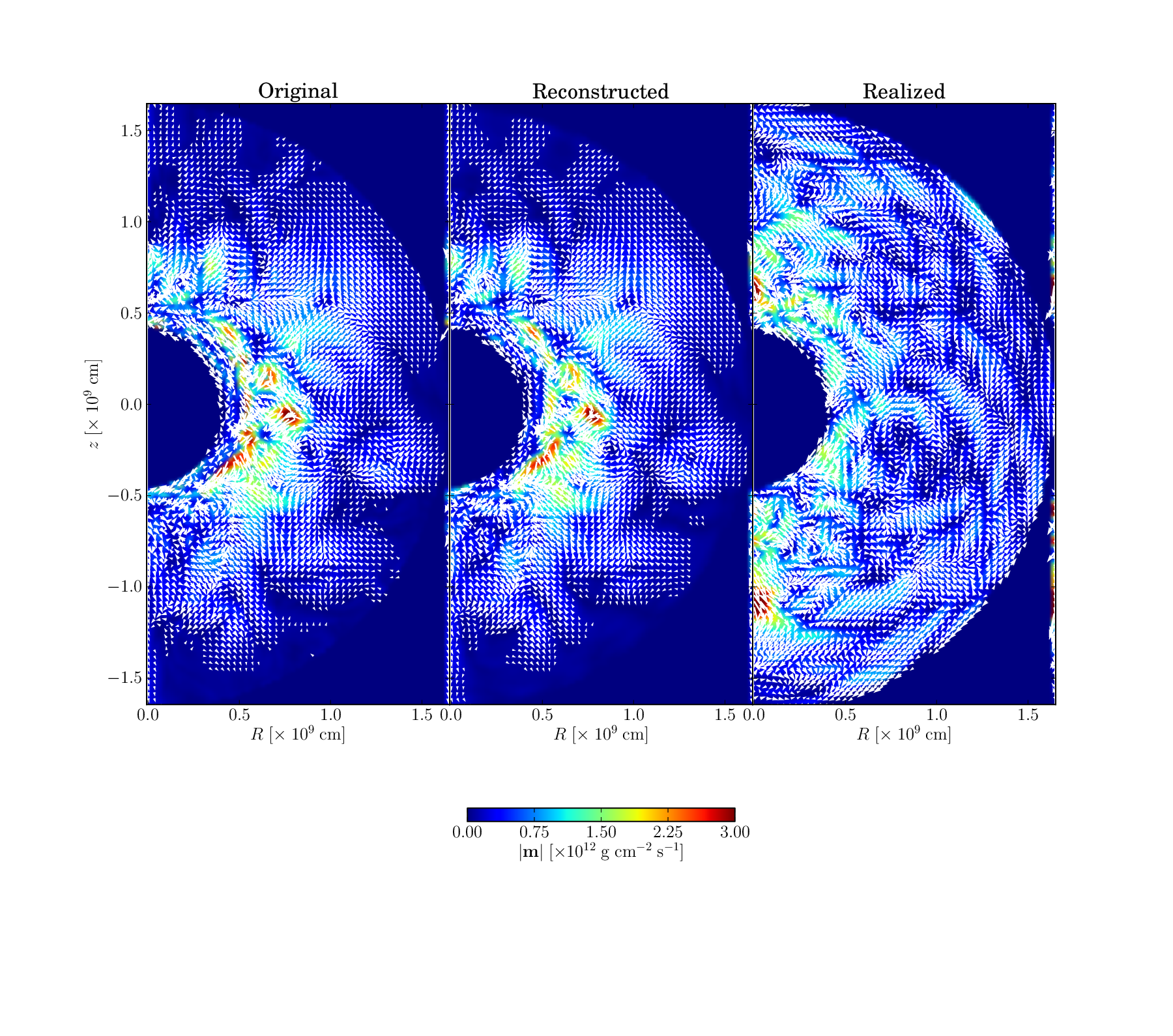
Another test of the VSH method is whether the original momentum density data can be recovered accurately by using the decomposition of Equations (12)-(15). Using the VSH decomposition of the convective oxygen-burning shell that we presented in Section III.1, we reconstruct the momentum density data using Equation (12). Figure 9 shows a comparison of the recovered (middle panel) versus the original (left panel) momentum density field. For the two datasets we calculate the L2-norm to assess the error of the reconstructed field using the formula:
| (23) |
We find 0.0029 indicating a successful reconstruction of the data within errors (since 1). Part of the residual deviation of the reconstructed momentum density field from the original one is due to the truncation of the sum over modes at , . Some of the residual is also attributable to the fact that at and the boundary conditions are not perfectly satisfied (see Section III).
III.2. Realization of simulation data from VSH power spectra.
An important application for the VSH framework presented here is the generation of non-spherically-symmetric initial conditions for CCSN simulations that include physically-motivated non-radial velocity fields. Inclusion of non-radial velocity perturbations to otherwise spherically-symmetric initial conditions has been shown to have an important qualitative impact on CCSN simulations [6]. This work, however, used very simplistic convolutions of sinusoids to perturb only the -direction velocity of the initial model. The scale and amplitude of these perturbations were chosen to resemble realistic multi-dimensional simulations of convective burning in CCSN progenitors near collapse, but this approach is ultimately insufficient to quantitatively capture the structure of convective velocity fields. Our method of VSH decomposition provides a far superior means of including non-radial velocity fields in the initial conditions for CCSN simulations. As discussed above, the VSH framework is purely kinematic in the sense that it includes no information about the physics that is producing the velocity field being considered, but it does respect appropriate boundary conditions for convective shells in stars. In this sections, we describe the process of realizing a pseudo-random velocity field from VSH spectra.
Under the assumption that the spectral distributions , , are known we can create corresponding realizations of . For this, we need to restore the phase and the -dependence by random number generation so as to turn the power spectra back into full VSH transforms.
In order to do this, we observe that since the data is real, the expansion coefficients in Equations (13)–(15) have the property , , – this is traceable to the relation which is inherited by the mode functions , , . It follows that for each mode, the process of extracting the spectral coefficients , , according to Equations (16)–(18) has elided the sign of the term (which is purely real) and the phases of the terms. The remaining terms are related to the terms by complex conjugation. We may therefore focus on realizing the truly independent real terms for each mode, and obtain the terms by complex conjugation.
Setting the components of a -dimensional vector by
| (27) |
it is clear that Equation (24) is satisfied when , that is, when is restricted to a unit hypersphere in dimensions. We may therefore realize a velocity distribution that respects the spectral distributions by constructing, for each , a random vector on this sphere.
Sampling such a random vector is a straightforward matter. We sample standard normal variables , . We then compute the normalization . Since the density function of the -dimensional multivariate normal distribution depends only on , the normalized random variables are distributed uniformly on the unit hypersphere in -dimensions, as required. The realized values of may be easily recovered from Equation (27). This procedure may obviously be repeated to obtain realizations of the spectra and . Of course, statistically-independent random number drawings should be performed for each of the three sets of modes. Once all (, , ) full power spectrum coeffiecents have been recovered, Equation 12 can be used to obtain the final realized momentum density field.
We note that for 2D momentum density data the realization process is different since only the mode is present, which is only uncertain up to a sign. In this case the random variables are drawn from a uniform distribution instead of a normal one, and are assigned a positive or a negative unity value according to whether they fall in the (0-0.5] or the (0.5-1] range respectively.
We use the VSH power spectra calculated in Section III.1 to produce a momentum density field realization by the process described above. The realized momentum density field for the O shell can be seen in Figure 9 (right panel) where it is compared with the original momentum density field (left panel). We observe that qualitatively, scales of macroscopic structures occurring in the original simulation also recur in the realized field.
It should be noted that the spectra only bear scale information, but do not carry any location information. This means that spatial structure such as stratification can be lost when is analyzed into modes and re-realized from the resulting spectrum. A stratified distribution with a quiescent core and a convective outer shell, spectrally-analyzed using whole-star modes and re-realized as above, will in general produce new momentum distributions with the same mix of scales as , but with no core-shell structure. If that structure must be preserved, it is necessary to divide the star into as many concentric layers as required, and analyze each layer separately. Nevertheless, the initial VSH decomposition requirements on mass, momentum conservation and boundary conditions (Equations 1-3) are already built in the method and the realization of phase information does not violate them. The conservation of mass flux, as we stated it in § II, is clearly visible in Figure 5, where the divergence-bearing mode () is clearly much smaller than the solenoidal modes.
More generally, realization by “restoring the phases” is a seemingly simple operation that is, however, fraught with physical significance. The VSH decomposition itself is, of course, purely a kinematic device, and nothing about the spatial coherence scales of the flow, such as might be determined by convective turbulence structures associated with time-domain intermittency, is included into the method. Depending on the distribution chosen to create randomly sampled phases, such flow structures can be realized or wiped out. Here we discuss a realization strategy in which the phases are all independent, identically distributed (IID) on the unit circle. This strategy is fully incoherent, and definitely wipes out any coherent spatial structure. This issue is clearly illustrated by considering the distribution of for the realized simulation as compared to the original data (red curve in Figure 4). Although the original and the realized radial components of the momentum density fields have a different spatial distribution, the average integrated value over the convective shell is very similar in the two. We return to a discussion of this issue in §V.
There is, as yet, no multi-dimensional simulation of the late stages of massive stellar evolution that ends at the point of core collapse in the literature. There are simulations, however, of convective Si shell burning in massive stars with iron cores [e.g., 2, Couch et al., in prep.]. As compared with detailed 1D CCSN progenitor models [38, e.g.,], these simulations typically make approximations such as reduced nuclear burning networks and replacement of the inner iron core by a boundary condition which make attaining core collapse difficult. Furthermore, these multi-dimensional simulations should not be regarded as fully deterministic as two similar simulations in identical progenitors that were subjected to different small scale perturbations in order to seed convection may result in well-developed convective structures that are not identical in phase. Until multi-dimensional CCSN progenitor models at the point of collapse are available, a step toward increased realism in CCSN simulations may be achieved be leveraging the VSH method we present here in conjunction with state-of-the-art 1D models.
The general procedure for constructing physically-motivated aspherical initial conditions for use in CCSN simulations would be as follows. First, a suitable simulation of convective burning prior to core collapse in the progenitor of interest is obtained. The structure of the velocity field in, e.g., the Si-burning shell surrounding the iron core is analyzed with the VSH framework and the spectra, Equations (16-18), are constructed. From the VSH spectra, we generate realizations of the velocity field using the procedure described above in this section which are applied to the Si shell of the 1D collapse model. This yields a vector velocity field with scale and structure statistically equivalent to the original convective burning simulation, in terms of the vector spherical harmonic information, but with a randomized phase. A goal of future work is to study whether or not the results of CCSN simulations are sensitive to the phase information of the convective velocity field in the Si shell at the time of collapse by conducting multi-dimensional CCSN mechanism simulations with several VSH-realized initial velocity fields that differ only in the random seed number of the phasing. A short-coming of this approach is the possibility for a small divergence of the evolution between the multi-dimensional convective burning simulation and that of the detailed 1D model. For our purposes, however, what matters most is accurately capturing the strength and scale of the convection in the moments prior to core collapse. We contend that the method sketched here should do just that and will result in initial conditions for CCSN that are more physically representative of real stars than anything that has been done before.
IV. APPLICATION TO THREE-DIMENSIONAL SIMULATION DATA
To apply the VSH decomposition method on 3D data we ran a 3D FLASH simulation featuring a 15- star O-burning shell on the Argonne Leadership Computing Facility (ALCF) Intrepid supercomputer using the same progenitor as for the 2D study. We used 83-zone blocks in a cm octant simulation box with reflective boundaries at the coordinate planes. The simulation used Cartesian coordinates and Adaptive Mesh Refinement (AMR), with a maximum resolution of 16 km. It was evolved for 430 s. Figure 10 shows a snapshot of the velocity magnitude at this latest simulated phase. Characteristic convective velocities of a few - cm s-1 are obtained, which are similar to the ones seen in the 2D simulation.

In order to obtain the correct VSH power spectra we constructed the full 4 steradian momentum density data using reflection symmetry about the three planes x-y, x-z and y-z. The radial coordinate and remain unaltered in all eight octants while the angular components of had either the same or an opposite sign depending on their specific octant. Of course, to recover the coordinates in the other octants we added multiples of while was the same for all octants in the northern hemisphere and for the southern hemisphere. Therefore the total number of zones in the O-burning shell for which we applied the VSH decomposition is eight times the number in the original octant simulation.
To compute power spectra with the large number of zones and modes in the 3D case, we implemented a parallelized computation of VSH in FLASH. Prior to doing so, we re-weighted the AMR Morton space-filling curve [36] to assign more weight to blocks residing in the O-burning shell, so that most processing power is focused on parts of the domain where it is needed. To reduce computational cost we also de-refined the AMR data outside the O-burning shell prior to applying the VSH decomposition. These three processes of parallelization, de-refinement of unused data and re-weighting of the Morton curve allowed us to efficiently compute 3D VSH spectra from within FLASH using the ALCF Mira supercomputer.
First, we determine the radial limits of the O-burning shell. The binned profiles of for several epochs are shown in Figure 11. The data shows that the radial component has a minimum at cm. We choose this value to be the inner boundary of the convective shell to be decomposed into VSH. For the outer boundary we investigate two values: a value that corresponds to the same as the inner boundary ( cm) and a larger value for which has even more significantly declined ( cm) in order to verify the robustness of the spectra under different choices of outer boundary.

We then run FLASH with the VSH implementation discussed above on 512 nodes (8192 cores) on Mira for 11.2 hours for a total of 91750 core hours per run. For these calculations we used 20 and 16 for a total of 7497 VSH modes calculated. Figure 12 shows the resulting reduced VSH power spectra in the case of the smaller (solid curves) and the larger (dashed curves) at 430 s. To properly compare the reduced VSH power spectrum in given the different shell sizes we express it in terms of the wavenumber in the right panel of Figure 12 using and . We find that choosing a larger outer radius does not significantly change the resulting VSH power spectra. We also show the evolution of the power spectra between 200 s and 430 s in Figure 13 as well as a time-averaged spectrum over these two phases (thick curves). While the slopes of the spectra remain consistent over time, considerable variance is observed for individual wavenumbers in accord with the 2D results. We see that the solenoidal modes dominate over the irrotational modes while the solenoidal modes are comparable to the irrotational modes. It is therefore still the case that more power goes to the solenoidal modes, but the solenoidal/irrotational power ratio is smaller than was the case in the 2D simulations. More specifically at 430 s in the 3D case, the total power of the two solenoidal modes together is g2 cm-1 s-2 while that of the irrotational mode g2 cm-1 s-2. We speculate that the increased importance of the irrotational flow with respect to the solenoidal flow is at least in part due to the physically unrealistic octant boundary conditions, which create radial-flow artifacts at the boundary planes. The lower resolution of the 3D simulation (16 km versus 8 km for the 2D simulation) may also contribute to the difference in power ratios.

Since the choice of a larger does not alter the VSH power spectra significantly we adopt the smaller value cm to calculate the final 3D convective O-burning shell VSH power spectra at two epochs: 200 s and 430 s for 15 and 11. The result is shown in Figure 12. We find that the slope of the solenoidal power spectrum in does not change significantly over this 230 s period in agreement with 2D results. However, the 430 s spectrum in this case peaks at 5 for both solenoidal modes and at 2. These peaks corresponds to characteristic angular scales cm and radial scales cm indicating that the convective elements tend to be oblately elongated in the tangential directions. Finally, these findings suggest that in 3D, convection in the O-burning shell moves more power to smaller radial scales but larger angular scales than in 2D. We also evaluated the exponential law slopes for the 3D power spectra at 430 s and recovered and accordingly for the - and -reduced spectra, indicating that the slope in is flatter than in the 2D case while the slopes in are consistent.

V. SUMMARY AND CONCLUSIONS
In this paper we present the method of Vector Spherical Harmonics (VSH) decomposition to characterize convective stellar velocity fields by calculating power spectra that yield information about the scales where convection has the most power, the distribution of convective power over those scales, and the shape of typical convective elements. We discussed our numerical implementation of the method and used it to calculate power spectra given a momentum density field from a simulation and the inner and outer radii of the convective region that we wish to decompose into VSH. We also discussed the techniques used to implement this method for use in large scale 3D simulations that can be used to analyze 3D FLASH AMR hydrodynamics simulations of stellar convection using large parallel computing resources, and can also be ported to other hydrodynamics codes.
We highlight the importance of properly characterizing multi-dimensional convection in pre-SN stars prior to initiating CCSN simulations. As previous studies have shown [21, 2, 3] the one-dimensional mixing-length theory for convection has difficulty in capturing the true nature of stellar convection in convective thin shell burning such as is expected in massive evolved stars. Vigorous convection in the oxygen shell during the core Si/S burning phase and in the silicon shell in the hours prior to iron core-collapse may significantly alter the structure of the progenitor star (Couch et al. 2014, in preparation). It can also affect the core-collapse dynamics and susceptibility to a successful explosion in 3D [6]. In addition, the large scale plumes that develop in realistic multi-dimensional convection in oxygen-burning shells can produce gravity waves that can lead to episodic mass-loss prior to the explosion, which affects the initial circumstellar environment within which the SN takes place [27, 28].
These results highlight that the core-collapse SN problem is an initial value problem, and that realistic 3D convective stellar velocity fields must be imposed on the progenitor models as initial conditions to hydrodynamic simulations [6]. We can use the VSH method to produce physically-motivated realizations of stellar velocity fields in the convective shells of SN progenitors using the derived VSH power spectra from multi-dimensional simulations, yielding more realistic, non-spherical initial conditions.
We have calculated the time evolution of reduced power spectra in both the angular (-modes) and the radial (-modes) scales for 2D and 3D convective oxygen shell burning of a 15- star. We have also used the 2D analysis and results to verify and test the predictions and accuracy of our method and to produce a realized 2D velocity field for the convective oxygen shell that bears the same scale information as the original field.
In connection with realization, however it is important to emphasize that the realization strategy that we implemented in §III.2 – with IID uniform phases – is in a certain sense naive, at least for some purposes. The point is that the VSH decomposition is a purely kinematic device, which does not incorporate any dynamical information a priori – all such information must be inferred by inspection of the VSH transforms. This distinguishes the method from approaches to convective turbulence such as Reynolds-averaging of the hydrodynamic equations [34], or the reduced-model approach based on ensembles of Lorenz convective rolls [3], where the dynamics are baked in to the analysis from the outset. One consequence of the dynamical agnosticism of the VSH transform method is that a choice of phase distribution (such as our IID uniform choice) can fail to reproduce the coherent spatial structure (such as convective rolls) that appear in the simulation from which the VSH transform was extracted.
The spatial coherence corresponding to dynamical flow structures characteristic of convective turbulence necessarily requires some kind of phase coherence. To reproduce it, the complex phases of the VSH transforms, as a function of , should be modeled by some distribution other than IID uniform. Those phases are of course available from the VSH transform. It would be interesting – and perfectly possible – to study them, and possibly even attempt to model them empirically using some correlated stochastic model, generalizing the naive IID uniform treatment of §III.2. If the distributional parameters of such a model were found to be in some sense statistically stable, we would have a further grip on the statistical description of the flow, above and beyond the statistically-stable properties of the spectrum. This possibility is a promising avenue of future research in stellar convective turbulence. Nevertheless, the velocity fields realized from VSH power spectra also obey to the requirements of the method on mass and momentum conservation as well as the proper boundary conditions. In the future we plan to investigate the sensitivity of CCSN explosion to phase restoration by random drawings using different seeds.
It is interesting to contrast the VSH characterization of a turbulent flow with the Karhune-Loeve (K-L) decomposition [31, 7], an established method for extracting the statistical content of such a flow. The K-L decomposition, which extracts the principal eigenmodes of the empirical kernel constructed from many relizations of the flow, is capable of exhibiting the principal coherent structures that are present in the flow, and indeed of correlating velocity field structure with attending structure in other field variables. The K-L decomposition therefore directly incoporates the phase-coherence modeling that would need to be added separately to the VSH decomposition, and therefore yields greater statistical information about the flow. In addition, for efficient decomposition, the kernel must be diagonalized by availing oneself of the problem symmetries. For box flows, this means Fourier transforms. In the spherical case of stars, the vector velocity component would necessarily have to be decomposed spherically, along the lines of a VSH decomposition. In summary, although the VSH decomposition method can itself be more computationally expensive than the K-L decomposition since it requires full multi-dimensional simulations and the calculation of a sufficient number of VSH modes it has it’s advantages with respect to the intended application to pre-SN stars with concentric convective shells.
An additional limitation of the VSH method derives from the fact that the velocity field, even at very low Mach number, does not fully characterize a turbulent flow. Pressure and density perturbation fields of comparable complexity to the velocity field are necessarily also present. We do not discuss the density perturbation field in this paper, but it may in fact play an important role in the core-collapse dynamics resulting from Pre-SN turbulence. For example, Meakin & Arnett [20] show that the largest density perturbations can occur at convective boundaries, whereas the implementation of the VSH decomposition developed here necessarily employs ”internal” boundary conditions, which protects the stratification but also eliminates the velocity fluctuations associated with density fluctuations at these boundaries. The effects of those fluctuations are therefore excluded from explosions that start from VSH realizations.
It is worth noting, in any event, that from the point of view of preparing CCSN progenitor models of greater realism than radial inflow models, the IID-uniform realizations may be perfectly adequate. There is no obvious specific reason why the difference between a spatially-coherent flow and a spatially incoherent one should be more important to the explosion properties of a CCSN than the difference between either of those and a radial flow.
We find that the slope of the VSH power spectrum of the solenoidal modes in does not significantly change over the time-scales we simulated with hints of power moving to different values of over time in both 2D and 3D. This illustrates an advantage of the VSH spectral decomposition: it furnishes a stable statistical description of the turbulent convection in a star.
We also find that most of the power goes to smaller radial and larger angular scales in 3D than in 2D. We determine the characteristic shape of the convective elements to be more asymmetric in 3D than in 2D. More specifically the convective eddies seem to be comparably elongated in the radial and tangential directions in 2D, while they seem to be “flatter” and more elongated in the tangential directions in 3D. We stress, however, that these results should not be over-interpreted, since the octant boundary conditions used in the 3D simulation result in axis-aligned artifacts that probably affect the spectral content of the flow, and since we simulated at most one convective overturn time-scale. We offer this analysis more as an illustration of the power of the VSH method, and of the kind of general observations about the nature of stratified convective flows that the method permits.
In the future we plan to use realized 3D convective fields obtained by the VSH decomposition method to initialize core-collapse simulations and investigate the effect of including more realistic initial conditions to the core-collapse problem. We also plan to use the method to analyze vigorous convective Si burning in the hours prior to core-collapse and study its evolution with time with the aim of understanding where most of the convective energy goes prior to collapse, and of investigating the convective shell properties of a variety of SN progenitors, including rotating and magnetized stars.
Appendix A DECOMPOSITION OF A GENERAL VECTOR FIELD INTO VSH MODES
A.1. Orthonormality and completeness.
The vector fields , are defined in terms of a generic Helmholtz equation solution . In order to furnish a full set of vector modes, it is necessary to specify a full Sturm-Liouville family of such solutions.
Accordingly, we adopt the orthonormal family of Helmholtz equation solutions
| (A1) |
where is a spherical harmonic function, and is a solution of the radially-separated Helmholtz equation,
| (A2) |
The superscript (“Dirichlet” and “Neumann”) on the function and on the eigenvalue refers to alternative sets of boundary conditions:
| (A3) |
and
| (A4) |
The discrete index on arises because the boundary conditions can only be satisfied for values in a discrete set. It is necessary to consider both sets of boundary conditions — Dirichlet and Neumann — because, as we will see, both types are required to create vector modes that satisfy the boundary condition of Equation (2).
The function is necessarily a linear combination of spherical Bessel functions of the first and second kind, and . The precise linear combination is dictated (up to a normalization) by the boundary conditions at and . The overall normalization is chosen so that
| (A5) |
The specific form of these radial functions is exhibited in the next section.
In terms of these modes, we define vector spherical modes patterned after the fields , of Equations (6–8). The irrotational mode is
| (A6) | |||||
where is a normalization constant to be determined. It is noteworthy and useful in what follows that the vector appearing in Equation (A6) is perpendicular to the radial direction, .
On careful examination, we can see that with the boundary conditions on and given in Equations (A3), (A4), is purely radial at the boundaries, whereas is purely tangential at the boundaries. By the physical boundary conditions on momenta (Equation 2) it follows that only the modes may be legitimately employed to represent stratified velocity fields. For whole-star () fields, on the other hand, both modes are available, and the appropriate mode should be selected depending on whether the velocity boundary condition at represents outflow or a tangential motion.
The first solenoidal mode is
| (A7) | |||||
Again, is a normalization constant. Both the Dirichlet and Neumann scalar functions are available, since manifestly neither leads to radial motion at the boundaries (or anywhere else, for that matter). Only one of the two sets should be selected, however. Recall that this mode represents a single degree of freedom (i.e. one scalar function) satisfying definite boundary conditions at and . Either mode set has the coverage to represent such a function. Given that the Dirichlet and Neumann modes aren’t even mutually orthogonal (see below), representing a vector field using both modes would be problematic, and certainly non-unique. The Dirichlet mode leads to velocity fields that are zero at the boundaries, so that if non-zero tangential motion at the boundary must be modeled, the Neumann modes are required. For this reason we will use the Neumann modes, setting by default.
The second solenoidal mode is
| (A8) | |||||
This can be expressed in terms of the elementary vectors and , using the identity :
| (A9) | |||||
where we’ve used the identity , the commutator , and the spherical Laplacian . Using the fact that , we obtain
| (A10) | |||||
It is clear from this expression that has a non-zero radial component at the boundaries, while is purely tangential at the boundaries. We therefore choose the Dirichlet modes as the mode set appropriate to the boundary condition of Equation (2). As we’ve now selected a scalar boundary condition for each mode set, we henceforth we drop the or subscripts from the mode vectors for convenience. From here on, , , and . The expressions for , , contained in Equations (A6), (A7) and (A10) correspond to those in Equations 13.3.67-69 of Morse & Feshbach [18].
It can be shown that all modes satisfy orthogonality relations. The are mutually orthogonal:
| (A11) |
where we’ve used boundary condition on , as well as the fact that . To confer unit norm upon the modes we thus choose
| (A12) |
The are also mutually orthogonal:
| (A13) |
It follows that has unit norm if
| (A14) |
It is straightforward to show that this orthonormalization would be unchanged had we selected Dirichlet modes instead of Neumann modes for .
Finally, the are mutually orthogonal as well:
| (A15) |
has unit norm if
| (A16) |
It can also be shown that each set is orthogonal to the other two:
| (A17) |
Thus the three sets of modes are all mutually orthogonal, and each of the , , represents a set comprising mutually orthonormal modes.
Completeness has not been established here. However, it is plausible to assume it. An arbitrary vector field corresponds in a sense to three scalar functions, each of which may be completely decomposed by sets of scalar functions such as the . Since we have deployed a set of such scalar functions in each of the three vector mode sets, the degree-of-freedom count is unvaried, and we should expect to be able to match arbitrary vector functions with these modes.
A.2. Boundary conditions: The Dirichlet and Neumann radial modes.
The Dirichlet radial mode functions satisfy the radially-separated Helmholtz equation
| (A18) |
subject to the boundary conditions (B.C.)
| (A19) |
As such, they are necessarily linear combinations of spherical Bessel functions of the first and second kind, and . It is straightforward to write down a combination that satisfies the B.C. at :
| (A20) | |||||
where is a normalization constant, and where for convenience we’ve introduced the notation
| (A21) |
The are the discrete, infinite set of roots of the equation
| (A22) |
obtained by imposing the boundary condition at on the solution of Equation (A20).
Using the properties of the spherical Bessel functions and the recursion relation (Arfken & Weber [1]):
| (A23) |
where stands for either or , it can be shown that the radial function normalization constant is given by
| (A24) |
The Neumann mode functions also satisfy Equation (A18), but with boundary conditions
| (A25) |
We may write down a linear combination of and that satisfy the boundary condition at :
| (A26) |
where the derivative terms were replaced using the recursion relation (Equation A23).
The are therefore the infinite set of discrete roots of the equation
| (A27) |
Using the relation of Equation (A23) this becomes
| (A28) |
and the normalization constant
| (A29) |
Equations (A22) and (A28) are oscillatory and have countably infinitely many roots, , that interleave with extrema that, in turn are roots of the derivatives of these equations. Our code uses the Newton-Raphson method to determine all roots and extrema in succession from 0 to where is given by Equation 19 (§II).
A.3. Dependence on vector field dimensionality and simulation domain.
There are fundamental differences in calculating VHS using 2D versus 3D vector field data. In the 2D case there is no need to evaluate the 0 modes because there is no information in the direction and rotational symmetry can be assumed (all terms are zero). Therefore only the , , and modes are calculated. In such case the convective elements can be thought as having a toroidal shape in 3D. As a result the total number of modes calculated is only .
In addition, one has to be careful about the 2D vector field data set used to calculate VHS in order for orthonormality to be established. The 2D data set needs to include data representing the whole volume of the convective shell and not just a quadrant portion (with polar angle ). Omission of half of the data will lead to erroneous treatment of orthonormality for the odd numbered (in ) irrotational modes and the even numbered (also in ) solenoidal modes. Therefore, if only quadrant 2D simulation data are available a full reconstruction of the data assuming symmetry by is necessary prior to the calculation of VSH. Similarly, in 3D octant simulations a full reconstruction of all data (full sphere) needs to be done assuming symmetry relations prior to the calculation of VSH power spectra.
References
- [1] Arfken, G. B., & Weber, H. J. 1995, San Diego, New York: Academic Press, —c1995, 4th ed.
- [2] Arnett, W. D., & Meakin, C. 2011, ApJ, 733, 78
- [3] Arnett, W. D., & Meakin, C. 2011, ApJ, 741, 33
- [4] Chandrasekhar, S. 1961, Hydrodynamic and hydromagnetic stability, International Series of Monographs on Physics, Oxford: Clarendon, 1961.
- [5] Chen, K.-J., Heger, A., & Almgren, A. 2012, arXiv:1204.4842
- [6] Couch, S. M., & Ott, C. D. 2013, ApJL, 778, L7
- [7] Deane, A. E., & Sirovich, L. 1991, J. Fluid Mech., 222, 231
- [8] de Jager, C., Nieuwenhuijzen, H., & van der Hucht, K. A. 1988, A&A Suppl., 72, 259
- [9] Dubey, A., Reid, L. B., Weide, K., et al. 2009, arXiv:0903.4875
- [10] Eggenberger, P., Meynet, G., Maeder, A., et al. 2008, Ap&SS, 316, 43
- [11] Fernández, R., Müller, B., Foglizzo, T., & Janka, H.-T. 2014, MNRAS, 440, 2763
- [12] Gilet, C., Almgren, A. S., Bell, J. B., et al. 2013, ApJ, 773, 137
- [13] Heger, A., Langer, N., & Woosley, S. E. 2000, ApJ, 528, 368
- [14] Jackson, J. D. 1975, 92/12/31, New York: Wiley, 1975, 2nd ed.
- [15] Kaniel, S., & Kovetz, A. 1967, Physics of Fluids, 10, 1186
- [16] Margutti, R., Milisavljevic, D., Soderberg, A. M., et al. 2014, ApJ, 780, 21
- [17] Mauerhan, J. C., Smith, N., Filippenko, A. V., et al. 2013, MNRAS, 430, 1801
- [18] Morse, P. M., & Feshbach, H. 1953, International Series in Pure and Applied Physics, New York: McGraw-Hill, 1953
- [19] Meakin, C. A. 2006, Ph.D. Thesis
- [20] Meakin, C. A., & Arnett, D. 2007a, ApJ, 665, 690
- [21] Meakin, C. A., & Arnett, D. 2007, ApJ, 667, 448
- [22] Makarov, V. V., & Murphy, D. W. 2007, AJ, 134, 367
- [23] Moriya, T. J., Maeda, K., Taddia, F., et al. 2014, arXiv:1401.4893
- [24] Paxton, B., Bildsten, L., Dotter, A., et al. 2011, ApJS, 192, 3
- [25] Paxton, B., Cantiello, M., Arras, P., et al. 2013, ApJS, 208, 4
- [26] Press, W. H., Teukolsky, S. A., Vetterling, W. T., & Flannery, B. P. 1992, Cambridge: University Press, —c1992, 2nd ed.
- [27] Quataert, E., & Shiode, J. 2012, MNRAS, 423, L92
- [28] Shiode, J. H., & Quataert, E. 2014, ApJ, 780, 96
- [29] Simon, R. 1969, A&A, 2, 390
- [30] Smith, N., & Arnett, W. D. 2014, ApJ, 785, 82
- [31] Sirovich, L. 1987, Quarterly of Applied Mathematics, 45, 561
- [32] Timmes, F. X. 1999, ApJS, 124, 241
- [33] Timmes, F. X., & Swesty, F. D. 2000, ApJS, 126, 501
- [34] Viallet, M., Meakin, C., Arnett, D., & Mocák, M. 2013, ApJ, 769, 1
- [35] Vink, J. S., de Koter, A., & Lamers, H. J. G. L. M. 2001, A&A, 369, 574
- [36] Warren, M. S., & Salmon, J. K. 1993, Proc. Supercomputing 1993, Washington, D.C.: IEEE Computer Soc., 12
- [37] Weaver, T. A., Zimmerman, G. B., & Woosley, S. E. 1978, ApJ, 225, 1021
- [38] Woosley, S. E., Heger, A., & Weaver, T. A. 2002, Reviews of Modern Physics, 74, 1015
- [39] Young, P. A., & Arnett, D. 2005, ApJ, 618, 908