Models of rotating boson stars and geodesics around them: new type of orbits
Abstract
We have developed a highly accurate numerical code capable of solving the coupled Einstein-Klein-Gordon system, in order to construct rotating boson stars in general relativity. Free fields and self-interacting fields, with quartic and sextic potentials, are considered. In particular, we present the first numerical solutions of rotating boson stars with rotational quantum number and , as well as the first determination of the maximum mass of free-field boson stars with . We have also investigated timelike geodesics in the spacetime generated by a rotating boson star for , and . A numerical integration of the geodesic equation has enabled us to identify a peculiar type of orbits: the zero-angular-momentum ones. These orbits pass very close to the center and are qualitatively different from orbits around a Kerr black hole. Should such orbits be observed, they would put stringent constraints on astrophysical compact objects like the Galactic center.
pacs
02.70.Hm, 04.25.D-, 04.40.Nr, 95.30.SfI Introduction
Boson stars are localized configurations of a self-gravitating complex scalar field, introduced in the end of the sixties by Bonazzola and Pacini [1], Kaup [2] and Ruffini and Bonazzola [3]. Motivated by the facts that (i) boson stars are, at the fundamental level, the simplest self-gravitating configurations of “matter” and (ii) they can act as black hole mimickers [4], numerous studies of boson stars have been performed (see [5, 6, 7, 8] for a review). A recent impetus to the topic has been provided by the discovery of the Higgs boson at CERN [9], which proves the existence of fundamental scalar fields in Nature. In addition, the main paradigm of current primordial cosmology, the inflation, is generally based on a scalar field (the inflaton) [10]. Still in the field of cosmology, we note that many dark energy models also rely on a scalar field, such as the quintessence model [11].
Boson stars studies have explored a large parameter space [5, 6, 7, 8], by varying the scalar field’s self-interaction potential, the spacetime symmetry (static, axisymmetric rotating or dynamical configurations), the number of spacetime dimensions (2 to 5), the spacetime asymptotic (flat or AdS) or the theory of gravity (general relativity, Einstein-Gauss-Bonnet gravity, scalar-tensor gravity, etc.).
We consider boson star models with a minimal coupling of the scalar field to gravity. They are described by the following action 11 1 We use geometrized units, in which both Newton gravitational constant and the speed of light are set to unity: . We also use the convention for the spacetime metric signature.:
| (1) |
where is the Hilbert-Einstein Lagrangian of the gravitational field:
| (2) |
being the Ricci scalar associated with the spacetime metric , and is the Lagrangian of the complex scalar field :
| (3) |
The potential is assumed to depend on only (U(1) symmetry). The simplest choice for is that corresponding to a free field:
| (4) |
the constant being the boson mass. Boson stars built on (4) are called mini-boson stars [7], for their maximum mass is very small, except for extremely tiny values of [5]. To get massive boson stars, Colpi et al. [12] have added a repulsive self-interacting term of the type to the potential :
| (5) |
where is a positive constant. Important mass can then be reached in the limit . Another generalization of the potential has been proposed by Friedberg et al. [13]:
| (6) |
where is a constant, which corresponds to the value of the field in the degenerate vacuum state. The potential (6) authorizes localized configurations of solitonic type, i.e. that can exist even in the absence of gravity, which is not possible for a free field. A related alternative is based on a potential of the form [14]:
| (7) |
where and are two constants. The corresponding solutions in flat spacetime are called -balls (see e.g. [15, 16]).
Beside the choice of the potential , models of stationary and axisymmetric rotating boson stars are based on the following ansatz for the complex scalar field :
| (8) |
where are coordinates adapted to the spacetime symmetries (i.e. is the stationarity generator and the axisymmetry one), is a positive real function of and only, is a real constant and is an integer, called the rotational quantum number [17, 8]. Note that has to be an integer in order for the scalar field to be single-valued at and . The ansatz (8) has been introduced by Kaup [2] for (nonrotating case) and by Schunck and Mielke [18] for . It leads to stationary solutions for the spacetime metric.
The first (numerical) solutions for rotating boson stars in general relativity have been obtained by Schunck and Mielke in 1996 [18, 19], considering a free scalar field [i.e. given by Eq. (4)] and to , as well as , in Eq. (8); their study was limited to the weakly relativistic regime. The strongly relativistic regime has been tackled in the works of Ryan [20] ( self-interaction and approximation valid for ) and Yoshida and Eriguchi [21] (free field with and ). In particular, the latter authors have performed the first determination of the maximum mass of free-field rotating boson stars for . In 2004, Lai computed a full sequence for , thereby obtaining a maximum mass value, but his code suffered from regularity issues at the rotation axis. In particular the maximum mass for was significantly different from that obtained by Yoshida and Eriguchi and Lai’s results have not been published but in the PhD thesis [22]. In the present work, we confirm the value found by Yoshida and Eriguchi [Eq. (51) below]. In 2005, Kleihaus et al. [17] have computed rotating boson stars with the self-interacting potential (7) for , generalizing the rotating -balls models of Volkov and Wöhner [14] to the self-gravitating case. They extended the study to and to negative parity scalar fields (i.e. antisymmetric with respect to the equatorial plane ) in [23] and analyzed the stability of the configurations in [24]. For the sake of completeness, let us mention that Hartmann et al. have studied special cases of rotating boson stars in 5-dimensional spacetimes [25] (the boson field is then actually a doublet of complex scalar fields) by assuming that the two angular momenta (associated with the 2 independent planes of rotations in 5 dimensions) are equal. Their results have been extended recently to 5-dimensional Einstein-Gauss-Bonnet gravity [26]. Solutions in higher dimensions, with only one Killing vector, are obtained in [27, 28]. Recently Herdeiro and Radu [29] constructed rotating solutions containing, in addition to the scalar field, an event horizon. Their solutions are thus hairy black holes, which can be viewed as intermediate states between rotating boson stars and Kerr black holes.
In the present article, we have considered both free-field boson stars [potential (4)] and self-interacting-field ones, based on the potentials (5) and (6), with the rotational quantum number ranging from to . We have developed a new numerical code, based on a spectral method, to compute the solutions of the coupled Einstein-Klein-Gordon equations. We have also investigated the timelike geodesics in the obtained numerical spacetimes. To our knowledge, the determination of geodesics around a rotating boson star has never been performed before; only the case of geodesics around nonrotating spherically symmetric boson stars has been dealt recently by Diemer et al. [30], for a self-interacting potential which reduces to (7) in the weak field limit. The particular case of circular timelike geodesics around static boson stars with various types of self-interaction (free, , and solitonic) has been investigated also recently by Macedo et al. [31].
This article is organized as follows. In Sec. II, we present the field equations to be solved (Einstein-Klein-Gordon system) as well as the relevant global quantities. Section III focuses on models of nonrotating spherically symmetric boson stars, while Sec. IV presents the models with rotation, which are axisymmetric. In both cases a detailed description of the numerical method, based on spectral methods, is given. Various error indicators are also exhibited and discussed. Section V is devoted to the study of orbits of massive particles around boson stars. Circular orbits and zero-angular momentum one are discussed, the latter ones being computed via a numerical integration of the geodesic equation. Conclusions and perspectives are given in Sec. VI.
II Field equations and global quantities
II.1 Equations to be solved
Variation of the action (1) with respect to the spacetime metric leads to Einstein equation
| (9) |
where is the Ricci tensor associated with , and is the energy-momentum tensor of the scalar field:
| (10) |
Variation of the action (1) with respect to the scalar field results in the Klein-Gordon equation:
| (11) |
Given some choice of the potential , the field equations (9)-(11) are solved for , under the assumptions of stationarity and axisymmetry for the spacetime metric and the ansatz (8) for (which is compatible with the assumed spacetime symmetries).
In the following, we use the language of the 3+1 formalism (see e.g. [32, 33, 34]), denoting by the hypersurfaces of constant , by the timelike future-directed unit normal to , by the metric induced by on , by the lapse function and by the shift vector, the last two quantities being defined by the orthogonal decomposition of the stationarity generator: , with . The spacetime metric line element can then be written as
| (12) |
Note that for stationary and axisymmetric spacetimes that are circular (cf. Sec. IV.1), such as those of rotating boson stars with of the type (8), .
II.2 Global quantities
Via Noether’s theorem, the U(1) symmetry of the Lagrangian (3) yields the following conserved current [2, 3, 8]:
| (13) |
It is divergence-free: and its flux through a hypersurface gives the scalar charge or total particle number of the boson star:
| (14) |
where (compare e.g. with Eq. (4.4) of Ref. [36]). By plugging the ansatz (8) into (13), we get
| (15) |
so that (14) becomes
| (16) |
The spacetime symmetries lead to two other conserved quantities, expressed by the Komar integral of the related Killing vector. The first one, associated to the Killing vector is the gravitational mass of the boson star. While the original Komar expression invokes a surface integral of the gradient of the Killing vector, it can be rewritten as the following volume integral [see e.g. Eq. (8.63) of Ref. [32]]:
| (17) |
In the present case, . Using the expressions derived in Appendix A for , and [Eqs. (67), (69) and (73) respectively], we arrive at
| (18) |
The second spacetime symmetry, the axisymmetry, leads to the angular momentum . The Komar expression can be recast as [see e.g. Eq. (8.75) of Ref. [32]]
| (19) |
where stands for the Killing vector Now . Using expressions (69) and (72) for and , we get
| (20) |
Comparing with (16), we recover the quantization law for the angular momentum of a rotating boson star [18]:
| (21) |
II.3 Units and order of magnitude
As stated above, in this article we use geometrized units: and . From Eqs. (1)-(3) and the fact that has dimension , it is clear that , and hence , is dimensionless in these units. In non-geometrized units, the dimension of is actually (i.e. square-root of a force), so that has the dimension of a wave function, i.e. .
In view of (4) or (6), a natural length scale that appears in the problem is the boson reduced Compton wavelength22 2 In this section, we restore the ’s and ’s.:
| (22) |
The boson gravitational mass scale associated with is
| (23) |
where is the Planck mass. Note that in geometrized units, .
In the free scalar field case, the maximal mass allowed for a boson star is of order . As can be seen in Tab. 1, it leads to small masses, even if the scalar field has the same mass as the electron.
For the potential (5) the situation is different. Indeed one can show [12] that the maximal mass scales as . is the true coupling constant (see [12]). If one assumes that is close to one, it leads to a dramatic increase of the allowed masses as can be seen in Tab. 1. In particular, if the scalar field has the same mass as the electron, one can reach values comparable to the ones of supermassive black holes. Let us point out that the corresponding values of are then very large, in particular much larger than the value studied in this paper (see Sec. IV.6 where ). Similar considerations hold for the potential (6) and we refer the reader to [6] for more details.
| Scalar field mass | |||
|---|---|---|---|
| Mass free-field (in kg) | |||
| Mass potential with (in kg) | |||
| Value of |
III Spherically symmetric models
III.1 Equations
Spherically symmetric solutions are constructed by setting in the ansatz (8) and by demanding that the field modulus depends only on :
| (24) |
Note that according to Eq. (21), implies a vanishing angular momentum; the spherically symmetric solutions are thus nonrotating. The corresponding spacetime is static [while is not, as it is clear from (24)]. In particular, in Eq. (12). Note that, contrary to fluid stars, staticity does not imply that the boson stars have to be spherically symmetric, as demonstrated by the non-spherically symmetric static solutions obtained by Yoshida and Eriguchi [35]. This is due to the anisotropy of the scalar field energy-momentum tensor (10). Therefore the spherical symmetry of our models results from the assumption in (24).
Thanks to spherical symmetry, we may choose spatial coordinates such that where is a flat metric (isotropic coordinates). The metric line element is thus
| (25) |
The unknown functions are , and , which all depend only on and obey the system obtained from the Einstein equation (9) and the Klein-Gordon equation (11):
| (26) | |||
| (27) | |||
| (28) |
where (3-dimensional flat Laplacian in spherical symmetry) and .
The system is closed by demanding that, at spatial infinity, one recovers Minkowski spacetime. This implies that , and when .
The simplest potential is that of a free field, as given by Eq. (4). It is the only one considered in this section but more complicated examples are given in Sec. IV. At the lowest order in , all the potentials considered reduce to the free field one so that the following discussions always hold. The dominant part of the asymptotic behavior of Eq. (28) with replaced by (4) is obtained by setting and :
| (29) |
For , solutions to this equation are oscillating spherical Bessel functions, which do not decay fast enough to lead to configurations with finite total energy. On the other hand regular solutions for decay like and are admissible solutions to the physical problem. In the following, we will focus on this case, i.e. assume . When , one can anticipate that the field vanishes ().
III.2 Numerical code
The system (26)-(28) is solved by means of a Newton-Raphson iteration implemented in a C++ code built on the Kadath library [37, 38]. This library enables the use of spectral methods for solving a great variety of partial differential equations that arise in theoretical physics. The 3-dimensional space is decomposed into several numerical domains. In this particular case spherical shells are used. In the outer numerical domain, space is compactified by making use of the variable so that the computational domain extends up to spatial infinity. Spectral methods are used [39]: in each domain, the fields are described by their expansions onto a set of known basis functions (typically Chebyshev polynomials). The unknown are then the coefficients of the expansions and the resulting non-linear system is solved iteratively. Regularity near is ensured by using only even Chebyshev polynomials in the numerical domain that encompasses the origin (a more detailed discussion about regularity can be found in the case ; see Sec. IV.2).


Let us point out that an empty flat spacetime (, and ) is a trivial solution to the system (26)-(28). In order to avoid convergence to this solution, one demands that the value of the field at the center takes a given non-zero value:
| (30) |
In order to maintain the same number of equations than unknowns, is not treated as a fixed parameter of the solution but rather as an additional unknown. The code finds the appropriate value of so that the condition (30) is fulfilled. This obviously prevents the code from converging to the trivial solution.
The precision of the code can be assessed by checking the convergence of the value found for when the number of radial coefficients is increased. This is shown on the first panel of Fig. 1. The convergence is exponential as expected for a well-posed problem solved by spectral methods. Another indicator of the code accuracy is the identity between the Komar mass and the ADM mass of the solution. The Komar mass, expressed above by the volume integral (18), can be computed from the gradient of the lapse function on a 2-sphere at spatial infinity, while the ADM mass is given by the gradient of the conformal factor (see e.g. Eq. (4.15) of Ref. [36] for and Eq. (8.48) of Ref. [32] for ):
| (31) | |||||
| (32) |
where is the 2-sphere of constant coordinate . Stationarity implies that [40, 41]. This equality can be viewed as a manifestation of the virial theorem [42]. The second panel of Fig. 1 shows, for two different configurations, the difference between the two masses, as a function of the number of coefficients . Once again the difference goes to zero exponentially. The very last point for slightly deviates from the exponential behavior probably due to the fact that the Newton-Raphson iteration is stopped at a threshold of or to round-off errors.


III.3 Solutions
Some results regarding the spherical case are shown in Figs. 2-4. The configurations are computed with and a decomposition of space in 6 radial domains. Figure 2 shows the value of as a function of . One can see that there is a range of values of for which more than one configuration exist. There is a minimum value of for . Figure 3 shows the value of the gravitational mass as a function of . We recover the maximum mass found by Kaup [2]: (reached for ). Finally Fig. 4 shows the radial profiles of , and for a configuration close to the minimum value of , that is for . The results from Fig. 2-3 confirm the fact that when , the fields goes to zero, as does its gravitational mass.
IV Rotating boson stars
IV.1 Equations
In order to construct boson stars that depart from spherical symmetry and are rotating, one considers the ansatz (8) with . The obtained configurations are stationary, axisymmetric and circular, i.e. the 2-surfaces of transitivity of the spacetime symmetry group (the surfaces of constant in adapted coordinates) are orthogonal to the surfaces of constant [43, 36]. Thanks to the circularity property, we may use quasi-isotropic coordinates (also called Lewis-Papapetrou coordinates), in which and , so that the 4-dimensional metric line element reads (see e.g. [36, 44])
| (33) | |||||
The metric is thus entirely described by four functions of : , , and . Note that the spherically symmetric case treated in Sec. III is recovered for and .
The Einstein equation (9) leads to the following system (see e.g. [36, 44], taking into account that these references make use of ):
| (34) | |||||
| (35) | |||||
| (36) | |||||
| (37) |
where and
| (38) | |||||
| (39) | |||||
| (40) | |||||
| (41) |
(resp. ) is the 3-dimensional flat Laplacian (resp. 2-dimensional) applied to axisymmetric functions. denotes the scalar product of the gradients of and , with respect to the flat metric. The quantities , , and are related to the 3+1 decomposition of the energy-momentum tensor, as defined in Appendix A. Using Eqs. (74)-(77), we find the explicit form of the terms involved in the right-hand side of (34)-(37):
| (42) | |||||
| (43) | |||||
| (44) | |||||
| (45) |
The scalar field obeys the Klein-Gordon equation (11), which becomes, once the metric (33) and the ansatz (8) are used,
| (46) |
The system of equations is closed by demanding that one recovers empty flat spacetime at infinity, i.e. that , , , and when .
The main difference between the spherical and axisymmetric boson stars is a change in the topology of the field . Indeed, for regularity reasons, must vanish on the rotation axis ( or ). It follows that the shape of the scalar field is no longer spherical but rather toroidal. More precisely, close to the axis, the field behaves like . For this ensures regularity on the axis because all the divisions by that appear in Eqs. (44)-(46) are made possible. The case is slightly more subtle, especially concerning Eq. (46), for terms like may appear singular at first glance. However the potentially singular part in the left-hand side of Eq. (46) is and a direct computation enables to verify that the singularities cancel. On the right-hand side of Eq. (46), the term may seem problematic when vanishes only like . However it is known that on the axis (local flatness, cf. [36]) so that the term vanishes at least as , thus ensuring regularity, even in the case. The regularity near the origin is ensured by the basis decompositions used in the innermost domain, as discussed in IV.2.
IV.2 Spectral solver
Let us note that boson stars have some common features with a class of field solutions known as vortons and already studied by means of Kadath in a previous article [45]. In the vorton case, a complex field has the same geometry as the field. However, instead of being coupled to gravity there is a second complex field and the two interacts. Nevertheless, the numerical treatment of the vorton field and the boson field is very similar.
The axisymmetric boson stars are computed using the polar space of the Kadath library, where fields are given in terms of the coordinates. As usual, space is divided into several radial domains and extends up to spatial infinity. Real scalar fields, like the lapse , are expanded onto even cosines with respect to the angular variable . As far as the radial coordinate is concerned, standard Chebyshev are employed, except in the domain that encompasses the origin, for which only even Chebyshev polynomials are used. We will refer to such basis of decomposition as the even basis. Another basis is the odd basis, where odd sines are used with respect to and odd Chebyshev polynomials with respect to , near the origin. It is for instance easy to see that if a field is expanded onto the even basis, then a ratio like must be expanded onto the odd one. Let us mention that, due to the non-local nature of spectral methods, the use of those basis is valid throughout the innermost domain, no matter what its size is.
The metric fields , , and must be expanded onto the even basis. This can be understood by noting that in Eq. (33) must be a scalar field. The case of is different in the sense that the “true” scalar is the field itself. In other words, is only the harmonic of a genuine scalar field. It follows that must be expanded onto the even basis if is even but onto the odd one when is odd. This situation is the same as that for the field in the vorton case [45]. This choice of decomposition is also consistent with the regularity condition that must vanish like on the axis. For completeness, let us mention that the numerical code does not search directly for the fields , , and but rather works with the auxiliary fields appearing on the left-hand side of Eqs. (34)-(37) which are , , and .
The system is solved by means of Newton-Raphson iterative scheme. For each value of , the most difficult part consists in finding a first solution. Once this is done, can be slowly changed to construct the whole family of configurations. This is to be contrasted with the parameter , which is an integer and so cannot be modified in this manner. For each we proceed as follows. First we consider an initial guess for of the form
| (47) |
where , , and , and are three constants that can be freely chosen; they control the amplitude of the field and the shape of the toroidal configuration. The form (47) ensures that the regularity condition on the axis is fulfilled and that the field decays as expected at spatial infinity. As for the spherical case (cf. Sec. III.2), in order to avoid that the solver converges to the trivial solution , is treated as an unknown and one demands that the field takes a given non-zero value at some point in the equatorial plane (we have to choose since for ). In order to facilitate convergence, one also tries to work in cases where the scalar field amplitude is small and the metric close to Minkowski spacetime. As already stated, this should give a value of close to . After a few trials, it is usually possible to find a choice of , , , and that leads to an admissible solution, i.e. that converges to a solution with . For instance, choosing , , , and proved to be a valid choice for . Once again, this is done only once for each value of , the other solutions being found by slowly varying .
IV.3 Error indicators
In order to check the accuracy of the code, several error indicators can be defined. First, as in the spherical case (Sec. III.2), one can check whether the ADM and Komar expressions of the gravitational mass agree.
The second error indicator was first obtained by Bonazzola [46] and arises because of the presence of a 2-dimensional Laplace operator in Eq. (37). Using the associated Green function, one can show that the solution decreases fast enough if, and only if, the source term (i.e. the right-hand side of Eq. (37)) has no 2-dimensional monopolar contribution. This is equivalent to
| (48) |
This is the so-called GRV2 identity [47]. Let us mention that even if Eq. (36) does involve another operator, it does not lead to such condition. Indeed, the source being proportional to , it has, by construction, no monopolar term. In previous works, for instance in the Lorene/nrotstar code (see Appendix B of [36]), it was necessary to enforce the condition at each step of the iteration by modifying the source of Eq. (37). With Kadath, no such treatment is required. This is probably due to the fact that the system is solved as a whole and not by separating the various equations in terms of operators on one side and source on the other one.
The third error indicator regards the computation of the angular momentum introduced in Sec. II.2. It can be evaluated by means of the volume integral (20) with in quasi-isotropic coordinates. Let us call this value. An alternative way to compute is via the Komar surface integral, which can be written as (see e.g. Sec. 4.4 of Ref. [36])
| (49) |
where is the 2-sphere of coordinate radius . Let us call the numerical value of hence obtained. Note that thanks to the compactification of the last domain, belongs to the computational domain and both expressions can be computed directly. One can then check whether .


The error indicators are shown on the different panels of Fig. 5 for different spectral resolutions. By resolution, one means the number of points in both the radial and the angular dimensions (those numbers are thereafter kept identical). Results are shown for and and . More precisely, the first panel shows the error on the masses defined as . On the second panel the error on the GRV2 identity is plotted and defined as being , where is the part of Eq. (48) that contains the term and the remaining terms. The third panel of Fig. 5 shows the relative difference of the two expressions for the angular momentum. All the error indicators exhibit a similar behavior, that is a spectral convergence [39]: the error decreases exponentially and then saturates due to round-off errors. The error on the angular momentum seems to slightly increase at very high resolution. By looking separately at the convergence of and with the resolution, one can see that the error is dominated by the surface integral . In this case, the round-off errors are greater because of the multiplication by that appears in Eq. (49). Those errors accumulate which explains the increase of the error at very high resolution. This suggests that it is preferable to use the volume integral (20) to compute the angular momentum.
IV.4 Numerical results for a free scalar field
In this section numerical results for rotating boson stars with , , and and the free-field potential (4) are presented. The same numerical setting is used for almost all the computations. It consists in a decomposition of the 3-dimensional space into 8 spherical domains. The last compactified domain extends from up to infinity. In each domain, 21 coefficients are used for both coordinates and . For the most relativistic configurations in the cases and , up to 33 coefficients are used. The Newton-Raphson iteration is stopped at the threshold of . This setting has been chosen to ensure a good accuracy in all the quantities presented thereafter. However, in some cases, this is not the best possible choice. For instance, in the case , the boson stars have a much larger size than in the case and would benefit from using more extended domains. An extensive survey of the parameter space would require some fine-tuning of the numerical parameters to ensure convergence and is beyond the scope of this paper.
Global quantities are plotted in Fig. 6. The gravitational mass [Eq. (18)] and the total angular momentum [Eq. (20)] are plotted as functions of . The binding energy is also shown; it is defined by
| (50) |
with the particle number given by (16). Maximum mass configurations are observed for , and . The case is the Kaup limit discussed in Sec. III.3. For , we recover the value found by Yoshida and Eriguchi [21]:
| (51) |
The maximum mass for could not be determined in Ref. [21], but the lower bound was established, with the hint that the maximum mass was not far from it (cf. Fig. 3 in Ref. [21]). In agreement with this lower bound, we find here (cf Fig. 6)
| (52) |
There is little doubt that maximum masses also exist for but these configurations are difficult to get given our standard numerical setting. Note however that if such maximum mass stars exist, they have an ergoregion as shown in Fig. 6 and therefore are likely to be unstable (see Sec. IV.5).
In the case , a turning point is observed around , meaning that no solutions are found for smaller values of . This also implies that there are values of for which two different boson stars coexist. For , configurations with positive binding energy are observed; they are expected to be unstable.


Figure 7 shows quantities related to the value of the scalar field . More precisely, the first panel shows as a function of the maximum value of and the second panel shows the gravitational mass as a function of the radius at which the maximum value of is attained. This last plot illustrates clearly the fact that the boson stars size increases with . This effect is also seen on Fig. 8 where isocontours of the scalar field are shown, for , and , and for a fixed value of (). Fig. 8 also shows (last panel) the corresponding profiles of the scalar field along the -axis.


Figure 9 shows the effect of on the structure of the scalar field. It illustrates the fact that the configurations are more and more extended as approaches .


IV.5 Ergoregions
A highly relativistic rapidly rotating object can develop an ergoregion, i.e. a spacetime region where the Killing vector becomes spacelike; in more physical terms, this means that, in such a region, no observer can remain static with respect to asymptotically inertial observers, due to some strong frame dragging effect. This concept is well known for a Kerr black hole, for which, as long as the angular momentum differs from zero, an ergoregion exists outside the event horizon. The existence of ergoregions in some rotating boson star models has been demonstrated by Kleihaus et al. [23].
As found by Friedman [48], scalar field configurations are unstable in spacetimes with an ergoregion but no event horizon, the instability mechanism being linked to superradiant scattering. The timescale of the instability depends on the spherical harmonic azimuthal index of the perturbation: it is very large for [49] and smaller for [50]. Some authors have put forward the existence of ergoregions to eliminate boson stars as viable alternatives to black holes in rapidly rotating compact objects [51]. However no exact computation of the instability timescale for rotating boson stars has been performed yet. Accordingly, we shall consider configurations with an ergoregion as potentially ruled out from an astrophysical viewpoint, their exact status depending whether the instability timescale is larger or shorter than the age of the Universe.
The assumption that is spacelike (ergoregion definition) is equivalent to or, in view of the quasi-isotropic line element (33), to
| (53) |
The region defined by the above equation is topologically a toroid. The minimal value of is plotted in Fig. 10 for all the rotating configurations. When it is negative, an ergoregion exists. The first panel shows that ergoregions appear at approximately the same value of : for and for , and , the last two being indistinguishable. For larger than this critical value, the configurations are not sufficiently relativistic for an ergoregion to exist. Once again, the second panel shows that boson stars are more extended for higher values of , as can be seen with the increase of the radius of the minimum with . The third panel of Fig. 10 shows the isocontours of in a meridional plane of constant , for and . The ergoregion is located where the isocontours are dashed lines. One can note that never changes sign on the axis so that ergoregions have always the shape of a torus.


IV.6 Rotating models with self-interacting potentials
Having explored the free field, we turn now to scalar fields with some self-interaction, i.e. with terms beyond the mass one in the potential . A great variety of such potentials have been proposed in the literature (see the reviews [7, 8]). An exhaustive study of them is beyond the scope of this paper. We focus instead on two potentials mentioned in Sec. I: the one [Eq. (5)] and the solitonic one [Eq. (6)].
At lowest order the potentials (5) and (6) reduce to the free field one. The technique used to compute solutions follows from this property. One starts with one of the free-field solution and one slowly changes the potential to reach the desired value of the parameters [potential (5)] or [potential (6)]. This technique works better if the starting configuration corresponds to small values of the scalar field, i.e. for values of close to . The precision of the obtained configurations can be assessed by the error indicators presented in Sec. IV.3.
Let us first consider the potential (5). In geometrized units, the constant is dimensionless. We select , which is a representative value considered by Colpi et al. for their study of the nonrotating case [12]. The value of is chosen only for illustrative purposes and does not come from any physical motivation. In particular it does not lead to a very big increase of the maximum mass. We have computed sequences of rotating configurations for this model, for ranging from 1 to 4 ( is also shown). Figure 11 shows the resulting gravitational mass as a function of . As a check, for , we recover the maximum mass found by Colpi et al. [12] for : . For , we find the values given in Table 2.
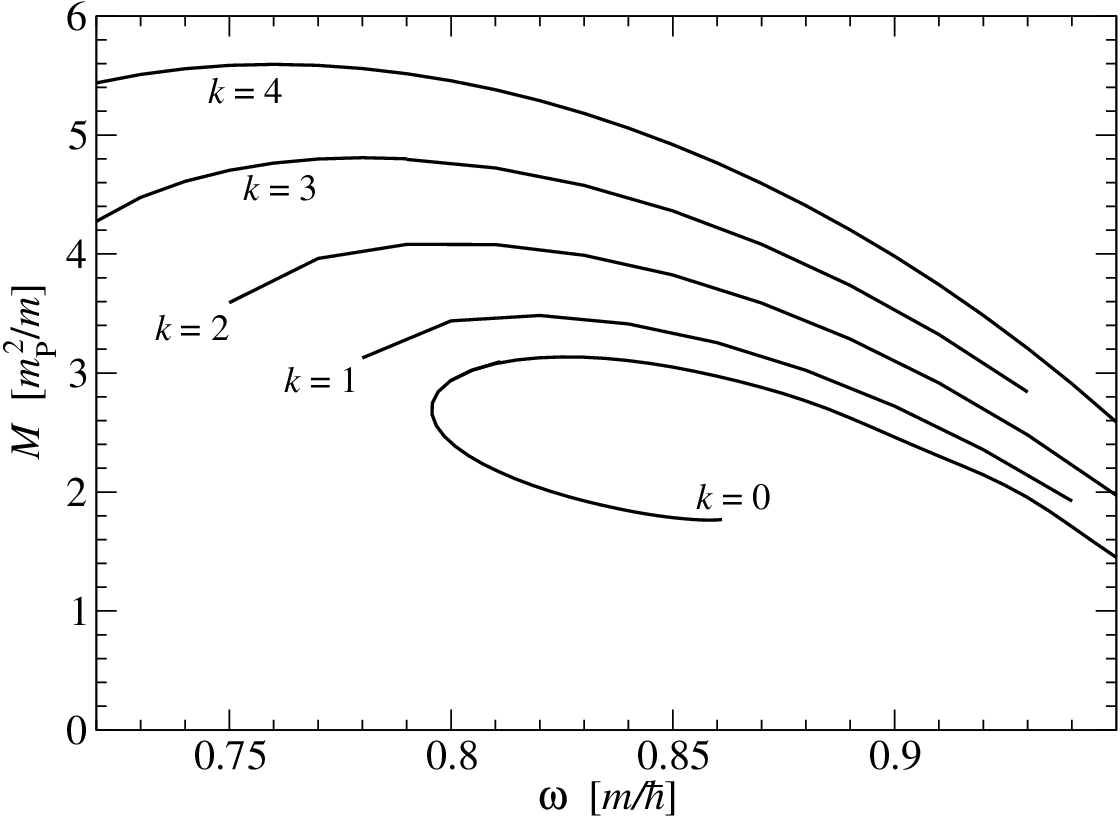
| 0 | 1 | 2 | 3 | 4 | |
|---|---|---|---|---|---|
| [] | 3.14 | 3.48 | 4.08 | 4.81 | 5.59 |
| [] | 0.83 | 0.82 | 0.80 | 0.78 | 0.76 |
For the solitonic potential (6), we perform the study for . As for potential this is only an illustrative value. Figure 12 shows the results regarding the gravitational mass . For solitonic boson stars, most of the previous works are concerned with relatively small values of , where a maximum mass is observed. For these configurations the scalar field is very close to a step function. Such a behavior is rather difficult to describe with spectral methods, for which smooth fields are required. Our code has therefore some difficulties in reaching very small values of . For moderate values of , our results are in good agreement with previous works. In particular, a secondary maximum is observed for near , as in Ref. [17].

This part of the article is not intended to constitute a detailed study of interacting potentials. It must rather be viewed as an illustration of the fact that our code is flexible enough to cope with various different situations. Comprehensive studies of the parameter space would however require some tuning of the various computational parameters. Let us eventually mention that no ergoregions have been found in the configurations presented in Figs. 11 and 12.
V Timelike Geodesics
A standard way to analyze a given spacetime geometry is to study its geodesics. Moreover computing geodesics leads to astrophysical observable. Being interested in the motion of stars in the vicinity of a supermassive boson star, we consider only timelike geodesics in this article, i.e. orbits of test particles of mass . In addition, we restrict ourselves to the equatorial plane () for simplicity. In this Section we consider only free-field boson stars, i.e. the models computed in Secs. III.3, IV.4 and IV.5.
The stationarity and axisymmetry of the underlying spacetime imply the existence of two constants of motion along any geodesic. Given the components of the particle’s 4-momentum with respect to the coordinates , these constants are expressible as and and are called respectively the particle’s energy “at infinity” and its angular momentum “at infinity”. The equation governing the variation of the radial coordinate along an orbit in the equatorial plane can be written as (see e.g. Ref. [36])
| (54) |
where is the particle’s proper time and the effective potential in the radial direction, , is given by
| (55) |
with and . Given (54), must be positive, which occurs if, and only if,
| (56) |
where and are the two roots of the equation
| (57) |
For any given value of , this second order polynomial equation in has for discriminant
| (58) |
which is always positive. Thus (57) does admit two solutions:
| (59) |
Here we may distinguish two cases. First of all, for boson stars without any ergoregion, the term in square brackets in Eq. (58), is always positive (compare to Eq. (53)), so that and is always negative. Since in the absence of ergoregion, one has always , we conclude that in this case, only the second inequality holds in (56). But, as discussed in Sec. IV.5, very relativistic rotating boson stars may have ergoregions. All signs are allowed for in these regions, so in this case we have to consider the two inequalities in (56). We treat these two cases separately in the next two subsections.

V.1 Effective potential outside ergoregions
To have a better understanding of the effective potential, we plot
as a function of for different values of
in Fig. 13. Each extremum of these curves
corresponds to a circular orbit.
We illustrate this fact in Fig. 14, which
is the reproduction of the Fig. 13 for a single value of
(). Indeed, we know that is constant
along the geodesic, so we choose an arbitrary value of
and represent it by an horizontal dotted line in Fig. 14.
The interval where gives the allowed
values of the radial coordinate (in Fig. 14, )
and the values of for which are turning
points, corresponding to the periastron and the apoastron. If we choose the energy of the particle to be equal to the
minimum of , only one value of the
radial coordinate is allowed (in Fig. 14 it corresponds to ):
this is a circular orbit.

We can infer two major facts from Fig. 13: first, all circular orbits around mini boson stars are stable, since they correspond to a minimum of the effective potential. Next, if we look at the behavior of particles approaching the boson star, we see that for , there is a infinitely high potential wall preventing the particle to reach . But for the particles with zero angular momentum (), we have a finite value for the energy at the exact center of the boson star. Note that we are assuming no interaction between the particle and the scalar field but the gravitational one, so that the particle may freely penetrate “inside” the boson star and reach its center.
V.2 Effective potential in ergoregions
As discussed in Sec. IV.5, rotating boson stars with ergoregions are unstable. If the (unknown) instability time scale in larger than the age of the Universe, then it is astrophysically relevant to study orbits around such stars, and in particular inside the ergoregion.
In the ergoregion, can be negative because in this part of spacetime the Killing vector associated with stationarity becomes spacelike. This is why in the ergoregion, we have to consider the two solutions (59). Accordingly in Fig. 15 we plot both and , for different values of and for a boson star that possesses an ergoregion. To develop an ergoregion, the boson star spacetime must be very relativistic and such configurations are obtained for small . For Fig. 15, we chose , along with the rotational quantum number . By “inverting” the reasoning made on Fig. 14, taking into account that , we may say that the maximum of corresponds to a stable circular orbits. These orbits, which exist only inside the ergoregion, are denoted by a dot in Fig. 15. We note also that inside the ergoregion, becomes positive in some range of for large enough.

V.3 Circular orbits
The two conditions satisfied by circular orbits are and , these two equations admit two solutions written here in terms of the circular orbit velocity with respect to the zero angular momentum observer or ZAMO (i.e. the observer of 4-velocity , cf. [52] and [36]), which is given by
| (60) |
with
| (61) |
is the velocity of the direct orbit and the velocity
of the retrograde one. For these solutions to exist we must have .
We solved numerically this inequality for many boson stars and
found that there is a minimum radius under which no circular orbit can exist.
Let us call the corresponding orbit the innermost circular orbit (ICO).
The value of its -coordinate depends on
the boson star as shown in Fig. 16. Let us point out that the ICO
is always located inside the torus.

Since and are velocities measured by a physical observer, the ZAMO, they must be subluminal, i.e. obey . This criterion is always verified for boson stars.
Let us discuss now in more details the stability of the circular orbits. Circular orbits are stable if, and only if,
| (62) |
If we plot for various boson stars,
as we do for four of them with fixed values of and
in Fig. 17, we see that this inequality is always strictly verified.
Thus, it seems that for rotating free-field boson stars, as long as a circular
orbit exists, it is stable.

We can compare these results to the black hole case (conditions for existence and stability of circular orbits are globally the same for Schwarzschild and Kerr spacetimes). For black hole spacetimes, circular orbits exist for larger than a critical value, so there is an ICO, located at for Schwarzschild spacetime. But the non-existence of circular orbits in certain regions of spacetime has a different cause for boson stars and black holes: for boson star this is due to becoming negative in the formula defining [Eq. (60)]. On the contrary, is always positive outside the horizon of a black hole. In this case, it is that is becoming larger than one beyond the ICO and thus prevent the existence of physical orbits. Moreover, the circular orbits around black holes, contrary to those around boson stars, are stable only for where ISCO stands for innermost stable circular orbit and corresponds to in Schwarzschild spacetime33 3 Let us recall that we are using isotropic coordinates, not areal ones; for the latter Schwarzschild ISCO is located at the well-known value .. For boson stars, we have found that, as long as a circular orbit exists, it is stable.
V.4 Zero angular momentum orbits ()
The orbits with zero angular momentum are interesting in the case of boson star because the particle is allowed to go through the star. This is not the case for black holes or ordinary stars, where a particle approaching towards the compact object faces either the event horizon or the stellar surface. Let us express the effective potential in the specific case . Equation (59) shows that is then equal to the lapse function:
| (63) |
We have plotted the profile of in Fig. 18
for different spherical () free-field boson stars. As noticed earlier, there is always
a stable equilibrium position at the center of the boson star. Then we consider rotating
boson stars, and in Fig. 19 we plot the effective potential for different
boson stars with a same value of () to compare with the
nonrotating case. We see that the equilibrium position still exists at
the center of the torus but has become unstable due to rotation. We
also note the existence of stable circular orbits close to the center
and remaining “inside” the boson star. In Fig. 20, we plot the
effective potential for boson stars with the same value of
but for different values of . The global behavior is the same
as in the previous figures but the scale enlarges as is increased.
This is consistent with the increase of the size of the torus with .


To fully determine the class of orbits, we used the GYOTO code [53, 54, 55] to integrate directly the geodesic equations within the 3+1 formalism [55], taking advantage of the capability of GYOTO to perform such an integration for a numerical metric. We first computed the the geodesic of a particle initially at rest in the spacetime of a nonrotating spherically symmetric boson star (). Due to spherical symmetry, the particle trajectory is a straight line. As expected, the particle go straight through the center of the boson star and oscillate back and forth, as it can be seen from Fig. 21, where we have plotted the particle’s -coordinate as a function of .

We repeated this calculation for a rotating boson star with and ,
still starting at rest from . The result is shown in
Fig. 22. We see clearly the manifestation of the Lense-Thirring
effect: the particle radially infalling is deflected near the center
and continues in almost a straight line before going backwards and
falling towards the center again. This gives rise to the
spike-like structure of the trajectory. Besides, this orbit is not closed.
In order to understand how these orbits are modified as the star’s rotational
quantum number is increased,
we plot the zero-angular-momentum orbit around boson stars with the
same value of as in Fig. 22
but with in Fig. 23
and in Fig. 24. We still see the characteristic
spikes, but the particle approaches less and less the center.
To investigate the behavior with respect to , we plot in
Fig. 25 a boson star with and
to compare with Fig. 23. We see that the effect of is to
change the value of the deviation angle when going through the
center.


We may call the orbits displayed in Figs. 22-25 the pointy petal orbits. Their spike-like structure is characteristic of boson star spacetimes, since the particle has to be able to move very close to the center to generate these orbits. This is indeed very different from the case of Kerr spacetime, in which all orbits are everywhere smooth and where a particle initially at rest always falls into the black hole.
VI Conclusions
We have developed a numerical code, based on multi-domain spectral methods, capable of solving the coupled Einstein-Klein-Gordon equations. We have used it to compute models of rotating boson stars, with various self-interacting potentials for the scalar field. We have obtained the first configurations with a rotational quantum number larger than , namely and . For , we have determined the maximum mass of a free-field boson star: , which was not known before. We have also confirmed the maximum mass found by Yoshida and Eriguchi [21]. For the self-interacting potential originally proposed by Colpi et al. [12], we have computed the first rotating models, with ranging from to and have determined the corresponding maximum masses (cf. Table 2).
We have also numerically computed timelike geodesics in rotating boson star spacetimes. In this article, we focused on circular orbits and zero-angular-momentum orbits. In particular, we have shown that as long as , there is an innermost circular orbit (ICO), i.e. a radius such that for no circular orbit exist. For , all the orbits are stable. We have found that circular orbits with zero angular momentum exist around boson stars, contrary to Kerr black holes. Moreover, we have exhibited a peculiar type of zero-angular-momentum orbits: the pointy petal ones. Such orbits do not exist in black hole spacetimes. Therefore observing them around some astrophysical system, such as the Galactic Center, would be a strong indication in favor of a rotating boson star for the central compact object.
In a future article [56], we shall perform a more systematic study of orbits around rotating boson stars, stressing the differences with black holes. In particular, it will be interesting to know if one can allow non-zero angular momentum and still observe “pointy petal orbits” exhibited in Sec. V.4. Preliminary studies seem to indicate that small but non negligible deviations in the value of are allowed.
Acknowledgements.
We warmly thank Silvano Bonazzola, Thibaut Paumard and Frédéric Vincent for useful discussions and advices. EG acknowledges the support from the ANR grant 12-BS01-012-01 Analyse asymptotique en relativité générale.Appendix A Energy-momentum tensor
Let us derive the explicit expression of the scalar field energy-momentum tensor resulting from the ansatz (8). First of all, (8) yields to the following components with respect to coordinates:
| (64) | |||||
| (65) |
We may then evaluate by means of the 3+1 expression of (see e.g. Eq. (5.51) of Ref. [32]), and get the explicit expression of the Lagrangian (3):
| (66) |
where the indices and take the values and only (i.e. label the coordinates ). Plugging (64)-(65) into (10) leads to
| (67) | |||||
| (68) | |||||
| (69) | |||||
| (70) | |||||
| (71) | |||||
| (72) |
where we have used the fact that and (circularity condition, cf. Sec. IV.1).
The trace of the energy-momentum tensor is obtained directly from (10):
| (73) |
The 3+1 decomposition of the energy-momentum tensor lets appear the energy density , the momentum density and the stress tensor , the three of them as measured by the ZAMO (i.e. the observer of 4-velocity ). These quantities are obtained as the following projections of :
with . Given the components (67)-(72) of and and , we get
| (74) |
| (75) |
| (76) |
The trace of the stress tensor, , has the following expression:
| (77) |
References
- [1] S. Bonazzola and F. Pacini, Phys. Rev. 148, 1269 (1966).
- [2] D. J. Kaup, Phys. Rev. 172, 1331 (1968).
- [3] R. Ruffini and S. Bonazzola, Phys. Rev. 187, 1767 (1969).
- [4] F. S. Guzman and J. M. Rueda-Becerril, Phys. Rev. D 80, 084023 (2009).
- [5] P. Jetzer, Phys. Rep. 220, 163 (1992).
- [6] T. D. Lee and Y. Pang, Phys. Rep. 221, 251 (1992).
- [7] F. E. Schunck and E. W. Mielke, Class. Quantum Grav. 20, R301 (2003).
- [8] S. L. Liebling and C. Palenzuela, Living Rev. Relativity 15, 6 (2012); [Online Article]: http://www.livingreviews.org/lrr-2012-6
- [9] ATLAS Collaboration, Phys. Lett. B 716, 1 (2012); CMS Collaboration, Phys. Lett. B 716, 30 (2012).
- [10] P. Peter and J.-P. Uzan, Primordial Cosmology, (Oxford Univ. Press, Oxford, 2012).
- [11] S. Tsujikawa, Class. Quantum Grav. 30, 214003 (2013).
- [12] M. Colpi, S. L. Shapiro, and I. Wasserman, Phys. Rev. Lett. 57, 2485 (1986).
- [13] R. Friedberg, T. D. Lee and Y. Pang, Phys. Rev. D 35, 3658 (1987).
- [14] M. S. Volkov and E. Wöhnert, Phys. Rev. D 66, 085003 (2002).
- [15] T. Tamaki and N. Sakai, Phys. Rev. D 81, 124041 (2010).
- [16] T. Tamaki and N. Sakai, Phys. Rev. D 83, 044027 (2011).
- [17] B. Kleihaus, J. Kunz, and M. List, Phys. Rev. D 72, 064002 (2005)
- [18] F. E. Schunck and E. W. Mielke, in Relativity and Scientific Computing, edited by F.W. Hehl, R.A Puntigam, and H. Ruder, (Springer, Heidelberg, 1996), p. 8.
- [19] F. E. Schunck and E. W. Mielke, Phys. Lett. A 249, 389 (1998)
- [20] F. D. Ryan, Phys. Rev. D 55, 6081 (1997)
- [21] S. Yoshida and Y. Eriguchi, Phys. Rev. D 56, 762 (1997).
- [22] C. W. Lai, A Numerical Study of Boson Stars, PhD thesis, University of British Columbia (2004); available as arXivgr-qc/0410040
- [23] B. Kleihaus, J. Kunz, M. List, and I. Schaffer, Phys. Rev. D 77, 064025 (2008).
- [24] B. Kleihaus, J. Kunz, and I. Schaffer, Phys. Rev. D 85, 024045 (2012).
- [25] B. Hartmann, B. Kleihaus, J. Kunz, and M. List, Phys. Rev. D 82, 084022 (2010).
- [26] Y. Brihaye and J. Riedel, preprint arXiv1310.7223
- [27] S. Stotyn, C.D. Leonard, M. Oltean, L.J. Henderson and R.B. Mann, Phys. Rev. D 89, 044017 (2014).
- [28] L.J. Henderson, R.B. Mann, and S. Stotyn, preprint arXiv1403.1865
- [29] C.A.R. Herdeiro and E. Radu, Phys. Rev. Lett. 112, 221101 (2014).
- [30] V. Diemer, K. Eilers, B. Hartmann, I. Schaffer, and C. Toma, Phys. Rev. D 88, 044025 (2013).
- [31] C. F. B. Macedo, P. Pani, V. Cardoso, and L. C. B. Crispino, Phys. Rev. D 88, 064046 (2013).
- [32] E. Gourgoulhon, 3+1 Formalism in General Relativity. Bases of Numerical Relativity, (Springer, Berlin, 2012).
- [33] T. W. Baumgarte and S. L. Shapiro, Numerical Relativity. Solving Einstein’s Equations on the Computer, (Cambridge Univ. Press, Cambridge, 2010).
- [34] M. Alcubierre, Introduction to 3+1 Numerical Relativity, (Oxford Univ. Press, Oxford, 2008).
- [35] S. Yoshida and Y. Eriguchi, Phys. Rev. D 55, 1994 (1997).
- [36] E. Gourgoulhon, An introduction to the theory of rotating relativistic stars, lectures given at CompStar 2010 School (Caen, 8-16 Feb 2010), available as arXiv1003.5015.
- [37] P. Grandclément, J. Comp. Phys. 229, 3334 (2010).
- [38] http://luth.obspm.fr/~luthier/grandclement/kadath.html
- [39] P. Grandclément and J. Novak, Living Rev. Relat. 12, 1 (2009); http://www.livingreviews.org/lrr-2009-1
- [40] R. Beig, Phys. Lett. 69A, 153 (1978).
- [41] A. Ashtekar and A. Magnon-Ashtekar, J. Math. Phys. 20, 793 (1979).
- [42] E. Gourgoulhon and S. Bonazzola, Class. Quantum Grav. 11, 443 (1994).
- [43] B. Carter, J. Math. Phys. 10, 70 (1969).
- [44] J. L. Friedman and N. Stergioulas, Rotating Relativistic Stars, (Cambridge Univ. Press, Cambridge, 2013).
- [45] P. Grandclément, G. Fodor, and P. Forgács, Phys. Rev. D 84, 065037 (2011).
- [46] S. Bonazzola, Astrophys. J. 182, 335 (1973).
- [47] S. Bonazzola and E. Gourgoulhon, Class. Quantum Grav. 11, 1775 (1994).
- [48] J. L. Friedman, Commun. Math. Phys. 63, 243 (1978).
- [49] N. Comins and B. F. Schutz, Proc. R. Soc. Lond. A 364, 211 (1978).
- [50] S. Yoshida and Y. Eriguchi: Mon. Not. R. Astron. Soc. 282, 580 (1996).
- [51] V. Cardoso, P. Pani, M. Cadoni, and M. Cavaglià: Phys. Rev. D 77, 124044 (2008).
- [52] J. M. Bardeen, Astrophys. J. 161, 103 (1970).
- [53] F. H. Vincent, T. Paumard, E. Gourgoulhon, and G. Perrin, Class. Quantum Grav. 28, 225011 (2011).
- [54] http://gyoto.obspm.fr/
- [55] F. H. Vincent, E. Gourgoulhon, and J. Novak, Class. Quantum Grav. 29, 245005 (2012).
- [56] C. Somé et al., in preparation.