Slowly Rotating Neutron Stars in Scalar-Tensor Theories
Abstract
We construct models of slowly rotating, perfect-fluid neutron stars by extending the classical Hartle-Thorne formalism to generic scalar-tensor theories of gravity. Working at second order in the dimensionless angular momentum, we compute the mass , radius , scalar charge , moment of inertia and spin-induced quadrupole moment , as well as the tidal and rotational Love numbers. Our formalism applies to generic scalar-tensor theories, but we focus in particular on theories that allow for spontaneous scalarization. It was recently discovered that the moment of inertia, quadrupole moment and Love numbers are connected by approximately universal (i.e., equation-of-state independent) “I-Love-Q” relations. We find that similar relations hold also for spontaneously scalarized stars. More interestingly, the I-Love-Q relations in scalar-tensor theories coincide with the general relativistic ones within less than a few percent, even for spontaneously scalarized stars with the largest couplings allowed by current binary-pulsar constraints. This implies that astrophysical measurements of these parameters cannot be used to discriminate between general relativity and scalar-tensor theories, even if spontaneous scalarization occurs in nature. Because of the well known equivalence between theories and scalar-tensor theories, the theoretical framework developed in this paper can be used to construct rotating compact stellar models in gravity. Our slow-rotation expansion can also be used as a benchmark for numerical calculations of rapidly spinning neutron stars in generic scalar-tensor theories.
pacs
04.50.Kd, 04.40.Dg, 97.60.Jd, 04.25.Nx, 04.30.DbI Introduction
Compact objects such as black holes and neutron stars (NSs) are ideal astrophysical laboratories to test the strong-field regime of general relativity (GR) [1, 2, 3].
The no-hair and uniqueness theorems [4] guarantee that astrophysical black holes in GR are the simplest macroscopic objects in nature, with structure and dynamics that are determined only by their mass and spin (but see [5] for a recent interesting counterexample). Therefore it is relatively easy (at least conceptually, if not in practice) to detect smoking guns of new gravitational physics by mapping the multipolar structure of a black-hole spacetime (see e.g. [6, 7, 8]) or by measuring the oscillation frequencies of black holes produced as a result of a compact binary merger [9, 10].
For NSs the situation is qualitatively different because of our poor understanding of the equation of state (EOS) of high-density nuclear matter. Different EOSs give rise to very different macroscopic NS properties, such as masses and radii. The growing wealth of NS observations holds great promise to constrain the EOS (cf. [11, 12, 13, 14] and [15] for a recent review), but the degeneracy between different EOS models and strong-field gravitational physics limits our ability to carry out tests of strong-field gravity. The reason is that uncertainties in our knowledge of the EOS are typically much larger than putative corrections from extensions of GR that are theoretically viable and pass weak-field tests.
This state of affairs has changed after the discovery by Yagi and Yunes ([16, 17]; see also [18]) that suitable dimensionless combinations of the moment of inertia , the tidal Love number and the spin-induced quadrupole moment of slowly-rotating NSs satisfy largely universal relations, where by “universal” we mean that these relations do not depend on the NS EOS within an accuracy of a few percent [19]. The universality is remarkably robust: various investigations showed that universal relations apply in GR also when the star rotates rapidly [20, 21, 22, 23], for moderately strong magnetic fields [24], and for stars whose parameters evolve dynamically due to interactions with a companion [25]. Various other nearly universal relations involving NSs have been discussed in the literature, and our understanding of the nature of these relations is steadily improving [26, 27, 28, 29, 30, 31]. The I-Love-Q relations are interesting for astrophysics because, if we assume that GR provides an accurate description of the strong-curvature regime, current and future observational facilities (e.g. ATHENA+ [32], LOFT [33], NICER [34] and the SKA [35] in the electromagnetic spectrum, as well as Advanced LIGO [36], Advanced Virgo [37], KAGRA [38] and the Einstein Telescope [39] in the gravitational-wave spectrum) may allow us to infer all three I-Love-Q quantities from the measurement of a single element of the triad (either , or ).
The existence of EOS-independent relations between the macroscopic parameters of compact stars in GR allows us, at least in principle, to circumvent the EOS-degeneracy problem mentioned above in the context of tests of strong-field gravity. Yagi and Yunes proposed the interesting possibility to constrain the underlying theory of gravity from measurements of the “no-hair like” I-Love-Q relations [16, 17]: if these relations are different in alternative theories of gravity (yet EOS-independent within each theory), then precision measurements of two of these quantities may allow us to discriminate between GR and possible extensions of the theory.
This is one of the most interesting applications of the I-Love-Q relations, but so far it has been explored only for two proposed alternatives to GR: Dynamical Chern-Simons (DCS) gravity [40] and Eddington-inspired Born-Infeld (EiBI) gravity [41, 42, 43]. For DCS gravity, it has been shown that tests based on the I-Love-Q relations can potentially constrain the theory better than current experimental bounds, basically because binary pulsar bounds on the theory are not very stringent [17]. On the other hand, the I-Love-Q relations in EiBI gravity were shown to be degenerate with their GR counterparts [44]. This degeneracy is interesting, but not surprising. EiBI gravity does not contain any extra degree of freedom with respect to GR. Solutions of the stellar structure equations in GR can be mapped to solutions in EiBI theory with an effective EOS [45] that is only slightly different from the corresponding GR EOS, given current experimental constraints on EiBI theory. For this reason, the indistinguishability of GR and EiBI theory is conceptually almost trivial. Furthermore there are issues with EiBI gravity, because the theory shares several of the pathologies that affect Palatini theories [46], including curvature singularities at the surface of polytropic stars and a problematic Newtonian limit [47].
In this work we investigate one of the most natural (and certainly the best studied) extensions of GR, namely scalar-tensor gravity [48, 1]. This is a fundamental theory with a well defined initial value problem [49] where gravity is mediated by the usual massless graviton and by a fundamental scalar field. The historical development of scalar-tensor theories was driven by a desire to investigate the role of Mach’s principle in gravity, but scalar degrees of freedom are ubiquitous in high-energy extensions of Einstein’s theory [50], in models that try to explain cosmological observations via modified gravity [51] and in inflation scenarios [52]. Certain classes of scalar-tensor theories are equivalent to gravity [53, 54]. Furthermore, scalar-tensor gravity can be considered as a simple phenomenological proxy for more complex strong-field extensions of GR.
In the context of NS physics, the interest in scalar-tensor gravity was revived after certain scalar-tensor theories were shown to produce “spontaneous scalarization” [55, 56]. In a nutshell, these theories allow for the same NS solutions as in GR, but the GR solutions become unstable beyond a critical central pressure and – in a phase transition akin to ferromagnetism – other solutions with a nonzero scalar charge appear. These “spontaneously scalarized” solutions are stable and can display relatively large deviations from their GR counterparts, even if the theory passes all weak-field tests [56]. This interesting phenomenon has been recently shown to be strengthened in dynamical situations, such as the final stages of a binary NS merger [57, 58, 59], and it has been shown to occur also for black holes surrounded by matter [60, 61].
Doneva et al. [62] recently studied scalarized configurations for rapidly rotating stars, showing that rotation enhances the effects of scalarization. The present paper is complementary to their work: we adopt the slow-rotation approximation (rather than solving the Einstein equations numerically for arbitrary rotation), but we extend the work of [62] by extracting all relevant physical quantities, including the quadrupole moment and the Love numbers, at second order in the slow-rotation expansion.
Our main result is that experimentally viable, spontaneously scalarized NS solutions have the same I-Love-Q relations as GR solutions within a few percent, i.e. the modified-gravity corrections are degenerate with the (small) deviations from universality within GR. Therefore, experimental measurements of the I-Love-Q relations cannot be used to distinguish GR from scalar-tensor theories, nor to put constraints on the latter that are more stringent than those currently in place [63].
These results, together with those for the very special case of EiBI gravity [44], suggest that – for most theories that are well constrained by weak-field tests – the modified I-Love-Q relations might be indistinguishable from their GR counterpart. On the other hand, our study proves that the I-Love-Q universality is remarkably robust even against beyond-GR corrections: as long as the modifications to GR affect both the strong- and weak-field regimes (and can therefore be strongly constrained by weak-field experiments), a measurement of one element of the triad can be used to infer the remaining two quantities within a few percent.
The paper is organized as follows. In Sec. II we present the main ingredients of our formalism to construct slowly-rotating NS configurations to second order in rotation in generic scalar-tensor theories of gravity. In Sec. III we focus on a theory that allows for spontaneous scalarization and we present our numerical results, showing that the universal I-Love-Q relations are very close to their GR counterparts for theories that are compatible with binary pulsar experiments. In Sec. IV we summarize the implications and possible extensions of our work. In Appendix A we present the field equations in the Einstein frame, and in Appendix B we discuss how to relate physical quantities in the Jordan frame to quantities computed in the Einstein frame.
II Framework
A generic class of scalar-tensor theories in the Jordan frame is described by the action [48]
| (1) | |||||
where is the Ricci scalar constructed out of the spacetime metric , is a scalar field, and collectively denotes the matter fields (which are minimally coupled to ). The constant is related to the physical gravitational constant (as measured in a Cavendish-type experiment), and from now on we will set it to unity together with the speed of light (see Appendix B for more details). Here and below we denote by a tilde quantities defined in the Jordan frame. Choosing the functions , and determines a specific theory within the class, up to a degeneracy due to the freedom to redefine the scalar [64].
By performing the transformations
| (2) |
the theory can be recast in the so-called Einstein frame, where the action reads
| (3) | |||||
In the Einstein frame the scalar field is minimally coupled to gravity, but the matter fields are minimally coupled to the metric , and nonminimally coupled to the conformal Einstein metric . The field equations in the Einstein frame read
| (4) | |||||
| (5) |
where the Einstein-frame stress-energy tensor is related to the physical (Jordan-frame) stress-energy tensor by
and the Jordan-frame stress-energy tensor for a perfect-fluid reads
| (6) |
We omit a tilde on the Jordan-frame pressure , density and fluid angular velocity , but since we only consider these quantities in the Jordan frame, the notation should not be ambiguous. To second order in , the fluid four-velocity reads , where
| (7) |
and is a bookkeeping slow-rotation parameter. In this paper all physical quantities characterizing the structure of a compact star will be expanded to . Note that
| (8) |
where, in the Einstein frame, with
| (9) |
so that . Because of the transformation of , the fluid angular velocity is the same in both frames: .
Following Hartle and Thorne [65, 66], the most general stationary axisymmetric metric to in rotation can be written as
where is a Legendre polynomial. The radial functions and are of zeroth order in rotation, and the related quantity (that will be useful below) are of first order, and , , , , are of second order. Under an infinitesimal rotation the scalar field, the pressure and the density all transform as scalars. As shown in [65, 66], in order to perform a valid perturbative expansion it is necessary to transform the radial coordinate in such a way that the deformed density in the new coordinates coincides with the unperturbed density at the same location. It can be shown that this transformation is formally equivalent to working in the original coordinates but expanding the pressure and the density as
| (11) | |||||
| (12) |
where we have assumed a barotropic EOS of the form . On the other hand, the scalar field is not affected by the fluid displacement and is simply expanded as
| (13) |
By plugging this decomposition into the gravitational and scalar-field equations (4)–(5) and by solving the equations order by order in we obtain a system of ordinary differential equations (ODEs).
We could in principle include a nonzero potential in these equations. While the inclusion of the potential is crucial in a cosmological context and can affect binary dynamics [67], for the present study of isolated compact objects we will assume that the scalar-field mass (and other self-interactions described by the potential) are small enough to be negligible, and we will focus on the case . The final form of the equations when is given in Appendix A. The more general equations for , along with the procedure to integrate the equations numerically and extract the relevant quantities (discussed below), are presented in a publicly available Mathematica notebook [68].
II.1 Integration of the field equations and extraction of the moment of inertia and quadrupole moment
The perturbation equations are very lengthy, and we summarize them in Appendix A. Schematically, the system can be written in the form
| (14) |
where
and is a 22-dimensional square matrix. The functions and are algebraically related to the others. This system of linear equations must be solved by imposing regularity at the center of the star, continuity at the surface, and asymptotic flatness at infinity. As we will discuss shortly, when we work at second order in rotation some of the equations are inhomogeneous, and the boundary conditions at infinity can be conveniently imposed using the corresponding homogeneous solutions, denoted by a superscript “(h)” in Eq. (). This is the reason why we integrate the full system (14), including both inhomogeneous and homogeneous quantities. The problem can be solved order by order in , but in practice it is more convenient to integrate all (zeroth-, first- and second-order) equations simultaneously.
Near the center, the leading-order behavior of the regular solution is
| , | ||
| , |
where , , and denote the values of the corresponding functions at the center of the star. Not all of the series expansion coefficients listed above are independent. Furthermore, to improve numerical stability, in our Mathematica notebook we included higher-order terms in the series expansions near the center. Without loss of generality, can be set to unity through a time rescaling, and can be set to unity by using the fact that the relevant ODE, Eq. (40), is homogeneous in . Since the gyromagnetic factor is linear in , at first order in rotation the entire family of spinning solutions can be obtained from a single element of the family by a suitable rescaling. Therefore, the first-order equilibrium structure is defined by two parameters: the central pressure and the central value of the scalar field .
Using the boundary conditions above, the system (14) can be integrated from to the stellar surface , defined by . By imposing continuity at the surface, all dynamical variables can be computed at , and the system can be integrated outwards from to infinity in the vacuum exterior, where . To zeroth order the quantity is fixed by requiring asymptotic flatness, i.e.
| (16) |
as , where is the mass of the star11 1 Since we integrate the equations derived from the action (3), all quantities are here defined in the Einstein frame. When presenting the results, however, we shall consider the corresponding quantities in the physical (Jordan) frame. The relevant transformations are discussed in Appendix B. Strictly speaking, only quantities in the Jordan frame can be observationally interpreted as the total mass, charge, angular momentum, etcetera: for example, the Jordan-frame mass is the quantity measured by applying Kepler’s law to weak-field orbits. and , where is the scalar charge of the star. For any fixed value of , we can determine the central scalar field that enforces asymptotic flatness through a shooting procedure. The angular momentum of the star is related to the asymptotic expansion of as follows:
| (17) |
The moment of inertia of the star is simply
| (18) |
and at leading order in the slow-rotation expansion it is independent of the NS spin (see [69, 23] for higher-order corrections).
Let us now discuss the boundary conditions for quantities of second order in rotation. Generic solutions of the inhomogeneous system are irregular at infinity, the general behavior being
| (19) |
where and are constants. The regular solution can be constructed by a suitable linear combination of a particular inhomogeneous solution and the corresponding homogeneous solution. The homogeneous system forms a two-parameter family, defined by the values of at the center. Without loss of generality, we construct two linearly independent solutions of the homogeneous system by choosing the values and for these parameters. A linear combination of these solutions is added to a particular solution of the inhomogeneous problem, and we choose the coefficients of the linear combination in order to cancel the divergent terms (19). A similar procedure is employed in the GR case [66]. The leading-order, large-distance behavior of the regular solutions reads
| (20) |
where is the spin-induced quadrupole moment of the star [66] and is a new quantity related to a quadrupolar deformation of the scalar field. A similar procedure is applied to compute the regular solutions and , whose asymptotic behavior reads and , where and are the second-order corrections to the total mass and to the total scalar charge, respectively.
II.2 Tidal Love numbers in scalar-tensor gravity
We compute the tidal Love numbers in scalar-tensor gravity by extending the relativistic formalism developed by Hinderer in GR [70], which in turn is based on the analysis of metric perturbations sourced by an external quadrupolar tidal field [71].
Restricting the analysis to , static, even-parity perturbations, a consistent ansatz is obtained from a subset of the decomposition in Eqs. ()–(12) by setting . After redefining , and , it can be shown that the field equations imply , and that the perturbation equations reduce to a coupled system of second-order ODEs:
| (21) | |||||
| (22) |
with
| (23) | |||||
| (25) | |||||
| (26) | |||||
where , and primes denotes derivatives with respect to the argument, i.e. and . As discussed in Appendix A, the variables and can be determined in terms of the other functions. As expected, the nonhomogeneous coefficients of the differential system depend only on zeroth-order (in ) background quantities, so that Eqs. (21) and (22) can be solved together with the original system (14), considering and as additional independent variables.
The regular solutions of Eqs. (21)–(22) near the center of the star behave as , , and higher order coefficients can be expressed in terms of and by solving the equations order by order near the center. We integrate the system twice with boundary conditions and at the center, respectively. By imposing continuity of , and their derivatives at the radius we construct two linearly independent solutions in the entire domain. Finally, we construct a linear combination of these solutions such that (as obtained by the linear combination) is regular at infinity, i.e. we impose the following asymptotic behavior for the linear combination of the two solutions:
| (27) | |||||
| (28) |
where the ’s and ’s are constants which can be expressed in terms of four independent parameters by using the field equations. The expression above is valid for , but it can be easily generalized to include a scalar potential. Finally, the tidal Love number is defined as [70]
| (29) |
We note that and that , , and are vanishing when the scalar charge . Therefore it is harder to extract the subdominant coefficient from a numerical solution when . Furthermore, the formalism allows us to extract also and , which is related to a quadrupolar deformation of the background scalar field. In analogy with the tidal Love number introduced above, we can define a scalar Love number (with dimensions of ) as follows:
| (30) |
II.3 relations and the slow-rotation approximation
Yagi and Yunes [16, 17] discovered that, within GR, the dimensionless quantities
| (31) |
( being the dimensionless spin) satisfy nearly universal relations that are insensitive to the NS EOS within an accuracy of the order of a few percent.
Another relevant quantity in the context of universal relations is the rotational Love number , which is related to the deformability of the NS away from sphericity due to its own rotation [72, 73]. The dimensionless quantity associated with this number can be expressed in terms of and as [17]
| (32) |
Our stellar structure equations correctly reduce to their GR counterparts [66, 74] when and , and we have tested our code by reproducing the results of Refs. [16, 17] in the GR case. As an additional test we have reproduced the results of Ref. [75] for the mass, radius, moment of inertia and quadrupole moment for several EOS models within GR.
It is important to remark that the universality discovered in [16, 17] can be affected both by observational uncertainties and by the slow-rotation approximation.
The normalizations in Eq. (31) involve powers of the mass of a nonrotating star (for and ) as well as powers of the dimensionless spin (for ). Astrophysical observations yield unbarred quantities, which must be normalized by the measured mass and (dimensionless) spin in order to satisfy EOS-independent relations. In the second-order slow-rotation approximation used here, the observable mass of a rotating NS is related to the mass of the nonrotating model by
| (33) |
where is the slow-rotation expansion parameter introduced earlier. The applicability of the universality relations to infer (say) and from will be limited in practice by measurement errors on and , not by the remarkably small dispersion between “barred” quantities. Since the normalization involves high powers of , small (say ) errors on the mass would translate into large () errors on . Similar considerations apply to the quadrupole moment, where the normalization is affected by both mass and spin measurement errors.
A related limitation in the practical use of I-Love-Q relations is that universality is effectively broken by a rotation-dependent term, because . For typical nuclear-physics motivated EOS and in the mass range of interest for NSs, (cf. e.g. [75], or Fig. 1 below). For millisecond pulsars the small rotation parameter can be as large as [76], so the difference between the rotating and nonrotating mass would introduce corrections to the universality which are of order , larger than the dispersion in the I-Love-Q relations themselves. While important in principle, this limitation is not of much concern in practice, for two reasons:
- 1)
The systems for which I-Love-Q tests would be astrophysically interesting include double pulsars, where precessional effects could lead to measurements of the moment of inertia [77], and compact binaries coalescences that may be observed by future gravitational-wave interferometers, allowing for measurements of the tidal Love number [74]. As argued convincingly in [16, 17], these systems typically involve NSs for which rotation rates are rather low.
- 2)
 |
 |
 |
 |
 |
 |
 |
 |
III Results
For concreteness, in our numerical integrations we focus on a theory defined by the action (3) with and
| (34) |
Isolated NSs in this theory were studied in Refs. [55, 56], where it was shown that GR solutions become energetically disfavored for sufficiently negative values of due to a phase transition (“spontaneous scalarization”) analogous to spontaneous magnetization in ferromagnetism. Therefore in some regions of the parameter space the theory admits stable NS configurations with nonvanishing scalar charge ().
In addition to the coupling parameter , the theory is also defined by the asymptotic value of the scalar field at infinity, . Binary-pulsar observations [63] require , whereas the measurement of the Shapiro time delay by the Cassini spacecraft [78] implies , where is related to the asymptotic value of the scalar field through [59]
| (35) |
Binary-pulsar constraints set even stronger bounds on when and, in fact, the upper bound on decreases very steeply as [63].
Using nuclear-physics based tabulated EOSs, we have computed slowly rotating NS configurations in this theory and extracted all relevant quantities to second order in the NS angular momentum. As a further test of our procedure, we have reproduced the results of Refs. [55, 56] for scalarized NSs to first order in the spin. The second-order results presented below are new. In our analysis we used three different EOSs covering a wide range of stiffness, namely FPS, APR, and MS1 (cf. e.g. Ref. [79] for a discussion of the models).
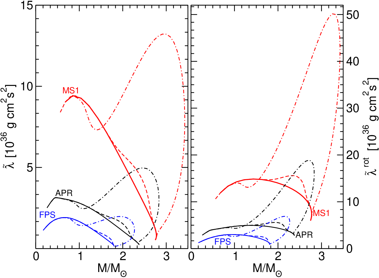
A summary of our findings is presented in Fig. 1. We perform numerical integrations in the Einstein frame, but all physical quantities shown in Fig. 1 refer to the physical (Jordan) frame, except for the mass which refers to the Einstein-frame Arnowitt-Deser-Misner mass (see Appendix B for details and for the relation between the two frames). The figure contains four panels. Each panel presents results for three models: (i) GR solutions (solid lines); (ii) scalarized solutions where the theory parameters are marginally excluded by binary pulsar experiments22 2 Recent unpublished observations of PSR J0348+0432 seem to exclude the region [80]. In order to maximize deviations from GR, we use very conservative parameters ( and ) for a marginally excluded scalar-tensor theory. The new observational bounds, if confirmed, would only strengthen our conclusions., i.e. and (dashed lines); (iii) scalarized solutions where the theory parameters violate current experimental bounds at more than confidence level [63], i.e. and (dash-dotted lines).
Above some critical value of the central pressure , the exact value depending on the EOS, scalarized solutions coexist with their GR counterpart. A linear perturbation analysis and numerical simulations of stellar collapse show that the domain of existence of the scalarized solutions coincides with the region where spherically symmetric GR solutions are linearly unstable and spontaneously develop a scalar charge [81, 82, 83]. The effects of scalarization are clear in the left inset of the top-left panel of Fig. 1, where we show the mass-radius diagram for the GR branch and for two scalarized theories. Rotationally induced mass corrections (shown in the right inset) are sensibly theory-dependent. The top-right panel shows the scalar charge (left inset) and rotationally induced corrections to the scalar charge (right inset) as functions of the stellar mass for scalarized solutions constructed using different EOS models. Corrections to the scalar charge can be very large, with for some values of the mass. This is consistent with the findings of Doneva et al. [62], who showed that rotation strengthens the effects of scalarization: roughly speaking, the total energy of the star must be large enough in order to scalarize, and scalarization is favored in spinning stars because of the rotational contribution to the total energy. The bottom-left panel shows that scalarization affects the moment of inertia (left inset) and the quadrupole moment (right inset). Finally, the bottom-right panel shows that tidal and rotational Love numbers are nontrivially modified by scalarization, with very large deviations in the case of theories that are already ruled out by binary pulsar experiments.
Although all quantities to second order in the spin display large modifications for different EOSs and also relative to GR, the behavior of the dimensionless quantities (31) turns out to be much more universal. In Fig. 2 we show the (left panels) and (right panels) relations for scalarized solutions. In the top panels, scalarized solutions refer to a theory with and ; in the bottom panels the theory parameters are and .
Let us first focus on the most relevant case, that of solutions that are only marginally disfavored by experiment (top panels). The top insets show six curves, corresponding to scalarized and nonscalarized solutions for three different EOSs, but these curves are indistinguishable on the scale of the plot: both in GR and in scalar-tensor theories, the I-Love-Q relations display very small deviations from universality. In general, the universal I-Love-Q relation will depend on our assumption on the correct theory of gravity: we can construct I-Love-Q relations either by fitting only pure GR solutions (middle inset in each panel), or by fitting only scalarized solutions (bottom inset). In the middle inset we show deviations from “pure-GR universality” for stars in GR (continuous lines) and for scalarized stars (dashed lines with symbols). Deviations from universal relations are typically of the order of or less for both and . Furthermore, the universal relations in experimentally viable scalar-tensor theories are very close to their GR counterparts.
One could have expected a priori that universal relations in scalar-tensor gravity would differ from those in GR, with larger deviations for larger absolute values of the coupling parameter . The top panels of Fig. 2 show that, even for a theory that is already marginally ruled out by binary-pulsar measurements, the I-Love-Q relations agree with those in GR within a few percent and, in fact, the deviation is comparable with the spread between different EOS models within GR. In order to assess the dependence on the coupling parameters, in the bottom panels of Fig. 2 we show results for a theory with and , that is already excluded by binary pulsar experiments at more than confidence level [63]. In this unrealistic case the residual from the GR universal relation can be as large as (cf. middle insets in the bottom panels Fig. 2), whereas within the scalarized theory the I-Love-Q relations are still nearly universal, as shown by the small residuals in the lower insets of the bottom panels.
For both scalar-tensor theories, the bottom insets highlight a rather interesting point: if we consider scalar-tensor theory as the correct theory of gravity, the deviations from a universal relation obtained by fitting numerical data within the theory are always very small. This means that the I-Love-Q relations are nearly universal, independently of whether GR or scalar-tensor theory is the correct theory of gravity. In other words, the universality is intimately tied to universal properties of matter, and it is quite insensitive to the dynamics of strong-field gravity.
 |
Finally, the dimensionless rotational Love number (32) is shown in Fig. 3 as a function of the stellar compactness for a scalar-tensor theory that is only marginally ruled out by binary pulsar experiments. As shown in the middle and lower insets, the residuals from a universal fit are smaller than , even for scalarized solutions. An interesting fact is that, contrarily to the cases shown in Figs. 1 and 2, the residuals of the scalarized solutions do not increase relative to the GR solutions, i.e. scalarization seems to affect the dimensionless rotational Love number even less than other quantities. A measurement of the NS mass and radius can be used to infer the rotational Love number even if the underlying theory of gravity is scalar-tensor theory.
In conclusion, the degeneracy between the I-Love-Q relations in GR and in scalar-tensor theories that allow for scalarization is a nontrivial fact. The degeneracy holds because of the tight experimental bounds imposed on scalarization by current binary pulsar experiments, and it is conceptually very different from the degeneracy observed in EiBI theory [44]. In that case, the degeneracy occurs because the theory does not contain any extra degree of freedom with respect to GR. As a consequence, perfect-fluid NS solutions in EiBI can be mapped to GR solutions with a different EOS [45]. The case discussed here is more interesting, because scalar-tensor theories propagate an extra scalar degree of freedom, so they are dynamically different from GR. Even at the mathematical level, all the equations that define the I-Love-Q relations depend explicitly on the background scalar field and, in turn, on the scalar charge . This result limits the prospects of performing strong-field tests of GR using I-Love-Q relations. On the plus side, it also means that astrophysical measurements of any of the three quantities (, or ) can be used to infer the other two, quite independently of assumptions on the EOS, as long as the underlying theory of gravity is well constrained by weak-field or binary-pulsar experiments.
IV Conclusions
We have presented a framework to construct slowly-rotating NSs in a generic scalar-tensor theory of gravity, extracting all relevant quantities to second order in the NS spin: mass, spin, scalar charge, moment of inertia, spin-induced quadrupole, tidal and rotational Love numbers.
We have focused on the simplest theory allowing for spontaneous scalarization [55, 56], but our equations (available online [68]) can be directly integrated in any scalar-tensor theory. In particular, our framework can be used to study NSs in gravity theories by virtue of their equivalence with scalar-tensor theories [53, 54].
We have found that the nearly universal I-Love-Q relations that were recently discovered in GR [16, 17] are very accurate (better than a few percent) for scalar-tensor theories that allow for spontaneous scalarization within current experimental bounds. Even for a theory that is already ruled out by observations, the universal relations agree with their GR counterparts within or less, whereas for a theory that is only marginally viable the deviations are lower than , i.e. comparable to the dispersion due to a different EOS within GR.
Our results imply that the simplest, best motivated and most-studied extension of GR cannot be distinguished from Einstein’s gravity using tests based on the I-Love-Q triad (cf. Ref. [44] for another example). On the other hand, our analysis tests the robustness of the I-Love-Q relations against beyond-GR corrections, showing that the relations derived in GR survive in scalar-tensor theories that are phenomenologically viable. This suggests that a measurement of one element of the I-Love-Q triad can be used to infer the remaining two quantities within less than a few percent, even adopting a relatively agnostic view on the behavior of gravity in the strong-curvature regime, which remains experimentally unexplored to date.
Finally, for a given scalar-tensor theory the dispersion from universality due to different EOSs is always smaller than a few percent, quite independently of the coupling parameters appearing in the action. This observation illustrates that the I-Love-Q relations remain EOS-independent in scalar-tensor gravity, and it seems to suggest that NS universal relations hinge more deeply on the “extrinsic”, global properties of ultra-stiff matter, rather than on the “dynamical” properties of the underlying gravitational theory.
In order to test these implications, it would be interesting to extend our study to other scalar-tensor theories. Examples include: (i) theories where the scalar field is massive, , which can evade weak-field tests [67, 84] and give rise to interesting strong-field effects, such as the existence of floating orbits [85]; (ii) tensor multi-scalar theories [86]; (iii) Horndeski theory [87, 50].
Another interesting avenue for future investigation is the extension of our study to universal relations between high-order multipoles in scalar-tensor theory. Studies in GR [23] show that high-order multipole relations have larger spread than the original I-Love-Q relations. Furthermore, high-order multipoles are harder to measure than low-order multipoles. For these reasons it seems unlikely that high-multipole relations will help in discriminating between scalar-tensor theories with spontaneous scalarization and GR better than the I-Love-Q relations. In any event, this is an interesting possibility that should be explored.
It will also be interesting to extend the second-order in rotation formalism developed here to other theories, such as Einstein-dilaton Gauss-Bonnet gravity: first-order calculations were carried out in [88, 89, 90], and recently extended to slowly-rotating black holes at second order in rotation [91], but (to the best of our knowledge) second-order calculations of stellar structure were not reported in the literature.
Finally, our results can be complemented and extended by constructing fast-rotating NS solutions in scalar-tensor theories (see [62] for work in this direction). This would allow us to verify whether the I-Love-Q universality in scalar-tensor theories is accurate enough for large rotation, as it seems to be in GR [20, 21, 22, 23]. In this context, the results of our slow-rotation study can be used as a benchmark and code test for full numerical solutions.
Acknowledgements.
We are grateful to Michael Horbatsch, Hector Okada da Silva, George Pappas, Kent Yagi and Nico Yunes for constructive criticism on an early draft of this paper. PP acknowledges the kind hospitality of the Harvard-Smithsonian Center for Astrophysics, where part of this work has been initiated. This work was supported by the European Community through the Intra-European Marie Curie contract aStronGR-2011-298297 and IRSES grant NRHEP 295189 FP7-PEOPLE-2011-IRSES, and by FCT-Portugal through projects IF/00293/2013 and CERN/FP/123593/2011. EB is supported by NSF CAREER Grant No. PHY-1055103.Appendix A Hartle-Thorne second-order equations for generic scalar-tensor theories
In this Appendix we present the field equations of a slowly-rotating, perfect-fluid star to second order in the angular momentum in scalar-tensor theories of gravity. We set for simplicity, but a more general form of the equations with can be found in a publicly available Mathematica notebook [68], together with the procedure to integrate the equations numerically (as explained in the main text).
Given the decomposition ()–(12) in the Einstein frame, the zeroth-order quantities are described by the following modified Tolman-Oppenheimer-Volkoff equations:
| (36) | |||||
| (37) | |||||
| (38) | |||||
The only first-order quantity is , which is described by a second-order ODE:
| (40) |
To , we obtain five first-order ODEs for , , , and ,
| (41) | |||||
| (42) | |||||
| (43) | |||||
| (44) | |||||
| (45) | |||||
and two second-order ODEs for and , that we write schematically as
| (46) | |||||
| (47) |
where the radial coefficients , and , as well as the source terms , are lengthy and unenlightening; their form can be found in the Mathematica notebook [68].
Using the other field equations, the right-hand side of Eq. (43) can be written as a total derivative and integrated, with the result
| (48) |
This expression reduces to Eq. (17b) in Ref. [66] in the GR limit . Finally, the functions and are algebraically related to the others through
| (49) | |||||
| (50) |
The equations for , , and are nonhomogeneous. As explained in the main text, the appropriate boundary conditions can be imposed with the help of the homogeneous equations, along the lines of the GR case [66]. We denote the solutions of the homogeneous equations as , , and , respectively. In reduced first-order form, we need to solve a system of 16 coupled ODEs plus six homogeneous first-order ODEs for , , and . The system can be written schematically as in Eq. (14).
Note that the equations at first order in rotation are a particular case of those presented in Ref. [90]33 3 We note here that the field equation in Ref. [90] contain some typos when , which are corrected in this paper and in the Mathematica notebook [68].. Here we have extended the analysis to second order, focusing on generic scalar-tensor theories.
Appendix B Transformations of the physical quantities to the Jordan frame
The field equations that we integrate numerically are derived from the Einstein-frame action of Eq. (3). In the Einstein frame, matter fields are nonminimally coupled with the conformal Einstein metric . However, laboratory clocks and rods measure the “physical” metric that appears in the Jordan-frame action of Eq. (1). In this Appendix we explicitly give the transformations relating the macroscopic properties characterizing NSs in the two frames.
Since the moment of inertia, the quadrupole moment and the tidal Love number all depend on the fall-off of the metric at large distances, once the asymptotic behavior of the Einstein-frame metric and of the scalar field are known, the Jordan-frame quantities can be easily computed from the asymptotic behavior of the Jordan-frame metric
| (51) |
where is defined in Eq. (13), and we recall that tilded quantities refer to the Jordan frame.
Because we imposed asymptotic flatness on the Einstein-frame metric, the conformal transformation (51) yields at infinity. In order for the Jordan-frame metric to be also asymptotically Minkowskian, we can simply rescale the time and radial coordinates: and . Note that, for phenomenologically viable values of , to a very good approximation, so this rescaling is practically negligible.
In addition, in scalar-tensor theories the effective gravitational constant (as measured by a Cavendish-like experiment) is not necessarily the same as the “bare” constant appearing in Eq. (1) (recall that we set in our Einstein-frame integrations). For the theory considered in the main text, where and is given by Eq. (34), the relation between these two quantities reads (see e.g. [59])
| (52) |
where for ease of notation we defined , and in the last step we have neglected the second term in square brackets, because it is negligible in the phenomenologically viable region of the parameter space. Thus, in the physical frame some coefficients of the large-distance expansion of the metric must be rescaled. For example, the Jordan-frame Arnowitt-Deser-Misner mass is obtained by comparing the asymptotic expansion of Eq. (51) with at large distances. By applying a similar procedure to the other components of we obtain
| (53) | |||||
| (54) | |||||
| (55) | |||||
| (56) | |||||
| (57) |
and
| (58) | |||||
Note that the moment of inertia is the same in both frames. This follows from the fact that and that also the fluid angular velocity, , is the same in both frames: . The transformation of the tidal Love number is more complex than the others because it depends on the expansion (27), whose subleading terms mix – through Eq. (51) – with the fall-off of the scalar field.
Since the issue about which frame should be considered “physical” in scalar-tensor theories is still debated (see e.g. [92, 64]) we have computed all quantities in both frames, with very similar results. All of the numerical results presented in the main text refer to the (measurable) Jordan-frame quantities, except for the mass. In theories that violate the strong equivalence principle the notion of mass is subtle. Following previous work (see e.g. [58, 62]), here we decided to present the Arnowitt-Deser-Misner mass in the Einstein frame , which coincides with the so-called tensor mass and has several desirable properties: it is positive definite, it decreases monotonically under gravitational-wave emission and it is well defined even for dynamical spacetimes [93].
References
- [1] C. M. Will, Living Rev.Rel. 9, 3 (2005), an update of the Living Review article originally published in 2001, arXiv:gr-qc/0510072 [gr-qc] .
- [2] D. Psaltis, (2008), arXiv:0806.1531 [astro-ph] .
- [3] N. Yunes and X. Siemens, Living Rev.Rel. 16, 9 (2013), arXiv:1304.3473 [gr-qc] .
- [4] P. T. Chrusciel, J. L. Costa, and M. Heusler, Living Rev.Rel. 15, 7 (2012), arXiv:1205.6112 [gr-qc] .
- [5] C. A. R. Herdeiro and E. Radu, (2014), arXiv:1403.2757 [gr-qc] .
- [6] F. Ryan, Phys.Rev. D52, 5707 (1995).
- [7] F. D. Ryan, Phys.Rev. D56, 1845 (1997).
- [8] D. Merritt, T. Alexander, S. Mikkola, and C. M. Will, Phys.Rev. D81, 062002 (2010), arXiv:0911.4718 [astro-ph.GA] .
- [9] E. Berti, V. Cardoso, and C. M. Will, Phys.Rev. D73, 064030 (2006), arXiv:gr-qc/0512160 [gr-qc] .
- [10] E. Berti, V. Cardoso, and A. O. Starinets, Class.Quant.Grav. 26, 163001 (2009), arXiv:0905.2975 [gr-qc] .
- [11] J. M. Lattimer and M. Prakash, Phys.Rept. 442, 109 (2007), arXiv:astro-ph/0612440 [astro-ph] .
- [12] F. Ozel, G. Baym, and T. Guver, Phys.Rev. D82, 101301 (2010), arXiv:1002.3153 [astro-ph.HE] .
- [13] A. W. Steiner, J. M. Lattimer, and E. F. Brown, Astrophys.J. 722, 33 (2010), arXiv:1005.0811 [astro-ph.HE] .
- [14] D. Psaltis, F. Ozel, and D. Chakrabarty, (2013), arXiv:1311.1571 [astro-ph.HE] .
- [15] M. C. Miller, ArXiv e-prints (2013), arXiv:1312.0029 [astro-ph.HE] .
- [16] K. Yagi and N. Yunes, Science 341, 365 (2013a), arXiv:1302.4499 [gr-qc] .
- [17] K. Yagi and N. Yunes, Phys.Rev. D88, 023009 (2013b), arXiv:1303.1528 [gr-qc] .
- [18] L. C. Stein, K. Yagi, and N. Yunes, (2013), arXiv:1312.4532 [gr-qc] .
- [19] J. M. Lattimer and Y. Lim, Astrophys.J. 771, 51 (2013), arXiv:1203.4286 [nucl-th] .
- [20] D. D. Doneva, S. S. Yazadjiev, N. Stergioulas, and K. D. Kokkotas, Astrophys.J. 781, L6 (2013a), arXiv:1310.7436 [gr-qc] .
- [21] G. Pappas and T. A. Apostolatos, Phys.Rev.Lett. 112, 121101 (2014), arXiv:1311.5508 [gr-qc] .
- [22] S. Chakrabarti, T. Delsate, N. Gurlebeck, and J. Steinhoff, (2013), arXiv:1311.6509 [gr-qc] .
- [23] K. Yagi, K. Kyutoku, G. Pappas, N. Yunes, and T. A. Apostolatos, (2014), arXiv:1403.6243 [gr-qc] .
- [24] B. Haskell, R. Ciolfi, F. Pannarale, and L. Rezzolla, (2013), arXiv:1309.3885 [astro-ph.SR] .
- [25] A. Maselli, V. Cardoso, V. Ferrari, L. Gualtieri, and P. Pani, Phys.Rev. D88, 023007 (2013), arXiv:1304.2052 [gr-qc] .
- [26] J. Lattimer and M. Prakash, Astrophys.J. 550, 426 (2001), arXiv:astro-ph/0002232 [astro-ph] .
- [27] L. Tsui and P. Leung, Mon.Not.Roy.Astron.Soc. 357, 1029 (2005), arXiv:gr-qc/0412024 [gr-qc] .
- [28] M. Urbanec, J. C. Miller, and Z. Stuchlik, (2013), arXiv:1301.5925 [astro-ph.SR] .
- [29] M. Baubock, E. Berti, D. Psaltis, and F. Ozel, Astrophys.J. 777, 68 (2013), arXiv:1306.0569 [astro-ph.HE] .
- [30] K. Yagi, Phys. Rev. D 89, 043011 (2014), arXiv:1311.0872 [gr-qc] .
- [31] M. AlGendy and S. M. Morsink, (2014), arXiv:1404.0609 [astro-ph.HE] .
- [32] D. Barret, K. Nandra, X. Barcons, A. Fabian, J.-W. d. Herder, et al., (2013), arXiv:1310.3814 [astro-ph.HE] .
- [33] E. Bozzo et al. (LOFT Consortium), EPJ Web Conf. 64, 09002 (2014), arXiv:1312.1697 [astro-ph.IM] .
- [34] K. C. Gendreau, Z. Arzoumanian, and T. Okajima, in Society of Photo-Optical Instrumentation Engineers (SPIE) Conference Series, Society of Photo-Optical Instrumentation Engineers (SPIE) Conference Series, Vol. 8443 (2012).
- [35] R. Smits, M. Kramer, B. Stappers, D. Lorimer, J. Cordes, et al., Astron.Astrophys. 493, 1161 (2009), arXiv:0811.0211 [astro-ph] .
- [36] Harry, G. M., for the LIGO Scientific Collaboration, Classical and Quantum Gravity 27, 084006 (2010).
- [37] Virgo Collaboration, Advanced Virgo Baseline Design, Virgo Technical Report VIR-0027A-09 (2009) https://tds.ego-gw.it/itf/tds/file.php?callFile=VIR-0027A-09.pdf.
- [38] K. Somiya, Classical and Quantum Gravity 29, 124007 (2012), arXiv:1111.7185 [gr-qc] .
- [39] M. Punturo, M. Abernathy, F. Acernese, B. Allen, N. Andersson, et al., Class.Quant.Grav. 27, 194002 (2010).
- [40] S. Alexander and N. Yunes, Phys.Rept. 480, 1 (2009), arXiv:0907.2562 [hep-th] .
- [41] M. Banados and P. G. Ferreira, Phys.Rev.Lett. 105, 011101 (2010), arXiv:1006.1769 [astro-ph.CO] .
- [42] P. Pani, V. Cardoso, and T. Delsate, Phys.Rev.Lett. 107, 031101 (2011a), arXiv:1106.3569 [gr-qc] .
- [43] P. Pani, T. Delsate, and V. Cardoso, Phys.Rev. D85, 084020 (2012), arXiv:1201.2814 [gr-qc] .
- [44] Y. H. Sham, L. M. Lin, and P. Leung, Astrophys.J. 781, 66 (2014), arXiv:1312.1011 [gr-qc] .
- [45] T. Delsate and J. Steinhoff, Phys.Rev.Lett. 109, 021101 (2012), arXiv:1201.4989 [gr-qc] .
- [46] E. Barausse, T. P. Sotiriou, and J. C. Miller, Class.Quant.Grav. 25, 062001 (2008), arXiv:gr-qc/0703132 [GR-QC] .
- [47] P. Pani and T. P. Sotiriou, Phys.Rev.Lett. 109, 251102 (2012), arXiv:1209.2972 [gr-qc] .
- [48] Y. Fujii and K. Maeda, ”The scalar-tensor theory of gravitation”, Cambridge University Press (2003).
- [49] M. Salgado and D. Martinez-del Rio, J.Phys.Conf.Ser. 91, 012004 (2007), arXiv:0712.2260 [gr-qc] .
- [50] T. P. Sotiriou, (2014), arXiv:1404.2955 [gr-qc] .
- [51] T. Clifton, P. G. Ferreira, A. Padilla, and C. Skordis, Phys.Rept. 513, 1 (2012), arXiv:1106.2476 [astro-ph.CO] .
- [52] J. Martin, C. Ringeval, and V. Vennin, (2013), arXiv:1303.3787 [astro-ph.CO] .
- [53] T. P. Sotiriou and V. Faraoni, Rev.Mod.Phys. 82, 451 (2010), arXiv:0805.1726 [gr-qc] .
- [54] A. De Felice and S. Tsujikawa, Living Rev.Rel. 13, 3 (2010), arXiv:1002.4928 [gr-qc] .
- [55] T. Damour and G. Esposito-Farese, Phys.Rev.Lett. 70, 2220 (1993).
- [56] T. Damour and G. Esposito-Farese, Phys.Rev. D54, 1474 (1996), arXiv:gr-qc/9602056 [gr-qc] .
- [57] E. Barausse, C. Palenzuela, M. Ponce, and L. Lehner, Phys.Rev. D87, 081506 (2013), arXiv:1212.5053 [gr-qc] .
- [58] M. Shibata, K. Taniguchi, H. Okawa, and A. Buonanno, (2013), arXiv:1310.0627 [gr-qc] .
- [59] C. Palenzuela, E. Barausse, M. Ponce, and L. Lehner, Phys.Rev. D89, 044024 (2014), arXiv:1310.4481 [gr-qc] .
- [60] V. Cardoso, I. P. Carucci, P. Pani, and T. P. Sotiriou, Phys.Rev.Lett. 111, 111101 (2013a), arXiv:1308.6587 [gr-qc] .
- [61] V. Cardoso, I. P. Carucci, P. Pani, and T. P. Sotiriou, Phys.Rev. D88, 044056 (2013b), arXiv:1305.6936 [gr-qc] .
- [62] D. D. Doneva, S. S. Yazadjiev, N. Stergioulas, and K. D. Kokkotas, Phys.Rev. D88, 084060 (2013b), arXiv:1309.0605 [gr-qc] .
- [63] P. C. Freire, N. Wex, G. Esposito-Farese, J. P. Verbiest, M. Bailes, et al., Mon.Not.Roy.Astron.Soc. 423, 3328 (2012), arXiv:1205.1450 [astro-ph.GA] .
- [64] T. P. Sotiriou, V. Faraoni, and S. Liberati, Int.J.Mod.Phys. D17, 399 (2008), arXiv:0707.2748 [gr-qc] .
- [65] J. B. Hartle, Astrophys.J. 150, 1005 (1967).
- [66] J. B. Hartle and K. S. Thorne, Astrophys.J. 153, 807 (1968).
- [67] J. Alsing, E. Berti, C. M. Will, and H. Zaglauer, Phys.Rev. D85, 064041 (2012), arXiv:1112.4903 [gr-qc] .
- [68]
http://blackholes.ist.utl.pt/?page=Files,
http://www.phy.olemiss.edu/~berti/research.html. - [69] O. Benhar, V. Ferrari, L. Gualtieri, and S. Marassi, Phys.Rev. D72, 044028 (2005), arXiv:gr-qc/0504068 [gr-qc] .
- [70] T. Hinderer, Astrophys.J. 677, 1216 (2008), arXiv:0711.2420 [astro-ph] .
- [71] K. S. Thorne and A. Campolattaro, Astrophys. J. 149, 591 (1967).
- [72] T. Mora and C. M. Will, Phys.Rev. D69, 104021 (2004), arXiv:gr-qc/0312082 [gr-qc] .
- [73] E. Berti, S. Iyer, and C. M. Will, Phys.Rev. D77, 024019 (2008), arXiv:0709.2589 [gr-qc] .
- [74] T. Hinderer, B. D. Lackey, R. N. Lang, and J. S. Read, Phys.Rev. D81, 123016 (2010), arXiv:0911.3535 [astro-ph.HE] .
- [75] E. Berti, F. White, A. Maniopoulou, and M. Bruni, Mon.Not.Roy.Astron.Soc. 358, 923 (2005), arXiv:gr-qc/0405146 [gr-qc] .
- [76] J. W. Hessels, S. M. Ransom, I. H. Stairs, P. C. C. Freire, V. M. Kaspi, et al., Science 311, 1901 (2006), arXiv:astro-ph/0601337 [astro-ph] .
- [77] J. M. Lattimer and B. F. Schutz, Astrophys.J. 629, 979 (2005), arXiv:astro-ph/0411470 [astro-ph] .
- [78] B. Bertotti, L. Iess, and P. Tortora, Nature 425, 374 (2003).
- [79] J. S. Read, B. D. Lackey, B. J. Owen, and J. L. Friedman, Phys.Rev. D79, 124032 (2009), arXiv:0812.2163 [astro-ph] .
- [80] N. Wex, private communication.
- [81] T. Harada, Prog.Theor.Phys. 98, 359 (1997), arXiv:gr-qc/9706014 [gr-qc] .
- [82] J. Novak, Phys.Rev. D57, 4789 (1998), arXiv:gr-qc/9707041 [gr-qc] .
- [83] P. Pani, V. Cardoso, E. Berti, J. Read, and M. Salgado, Phys.Rev. D83, 081501 (2011b), arXiv:1012.1343 [gr-qc] .
- [84] E. Berti, L. Gualtieri, M. Horbatsch, and J. Alsing, Phys.Rev. D85, 122005 (2012), arXiv:1204.4340 [gr-qc] .
- [85] V. Cardoso, S. Chakrabarti, P. Pani, E. Berti, and L. Gualtieri, Phys.Rev.Lett. 107, 241101 (2011), arXiv:1109.6021 [gr-qc] .
- [86] T. Damour and G. Esposito-Farese, Class.Quant.Grav. 9, 2093 (1992).
- [87] G. W. Horndeski, Int.J.Theor.Phys. 10, 363 (1974).
- [88] P. Pani and V. Cardoso, Phys.Rev. D79, 084031 (2009), arXiv:0902.1569 [gr-qc] .
- [89] P. Pani, C. F. Macedo, L. C. Crispino, and V. Cardoso, Phys.Rev. D84, 087501 (2011c), arXiv:1109.3996 [gr-qc] .
- [90] P. Pani, E. Berti, V. Cardoso, and J. Read, Phys.Rev. D84, 104035 (2011d), arXiv:1109.0928 [gr-qc] .
- [91] D. Ayzenberg and N. Yunes, (2014), arXiv:1405.2133 [gr-qc] .
- [92] V. Faraoni and E. Gunzig, Int.J.Theor.Phys. 38, 217 (1999), arXiv:astro-ph/9910176 [astro-ph] .
- [93] D. L. Lee, Phys.Rev. D10, 2374 (1974).