Abundance of Field Galaxies.
Abstract
We present new measurements of the abundance of galaxies with a given circular velocity in the Local Volume: a region centered on the Milky Way Galaxy and extending to distance 10 Mpc. The sample of mostly dwarf galaxies provides a unique opportunity to study the abundance and properties of galaxies down to absolute magnitudes , and virial masses . We find that the standard CDM model gives remarkably accurate estimates for the velocity function of galaxies with circular velocities and corresponding virial masses , but it badly fails by over-predicting times the abundance of large dwarfs with velocities . The Warm Dark Matter (WDM) models cannot explain the data either, regardless of mass of WDM particle. Just as in previous observational studies, we find a shallow asymptotic slope of the velocity function, which is inconsistent with the standard CDM model that predicts the slope . Though reminiscent to the known overabundance of satellites problem, the overabundance of field galaxies is a much more difficult problem. For the standard CDM model to survive, in the 10 Mpc radius of the Milky Way there should be not yet detected galaxies with virial mass , extremely low surface brightness and no detectable HI gas. So far none of this type of galaxies have been discovered.
Keywords:
cosmology: theory – dark matter – galaxies: halos – methods: N-body simulations.1 Introduction
The velocity function, which is defined as the abundance of galaxies with a given circular velocity, is one of fundamental statistical properties of galaxies. It is a kin of the much more well known and studied statistics: the luminosity function - the abundance of galaxies with a given luminosity. The luminosity function is easier to measure, and indeed there are numerous estimates of the luminosity function (Norberg et al., 2002; Bell et al., 2003; Blanton et al., 2005; Montero-Dorta & Prada, 2009, e.g.,). From the theoretical point of view there are substantial differences between luminosity and velocity functions. It is much more difficult to make theoretical predictions for the luminosities. Galaxy luminosity and stellar mass are the results of a complicated history of star formation of a galaxy. It depends on accretion and merging history and also on many other processes, which operate when a galaxy evolves – the stellar winds, supernovae explosions, galactic fountains – to name a few. This makes the luminosity and stellar mass very valuable tools to study the evolution of the Universe, but it makes them very difficult to predict.
Testing the theoretical predictions of the abundance of galaxies can done using the Semi-Analytical Models (SAMs) (White & Frenk, 1991; Somerville & Primack, 1999; Benson et al., 2003; Somerville et al., 2012, e.g.,). Unfortunately, SAMs use many assumptions and parameters, which make theoretical predictions somewhat uncertain. The main source of the uncertainty is due to the lack of detailed understanding of how galaxies form and evolve in the cosmological framework. Another popular way of relating dark matter halos with galaxies are the halo abundance matching (HAM) (Kravtsov et al., 2004; Conroy, Wechsler, & Kravtsov, 2006; Trujillo-Gomez et al., 2011) and the halo occupation distribution (HOD) (Berlind & Weinberg, 2002; Kravtsov et al., 2004; Zentner et al., 2005). These methods are often used to predict galaxy clustering at different redshifts. However, they assume galaxy luminosity or stellar mass functions, and thus cannot be used to test theory when it comes to predictions of abundances of galaxies.
Because the circular velocity measures the mass in the inner region of a dark matter halo (e.g., about for a Milky-Way mass halo) where the observed galaxy is situated, and because the circular velocity does not depend on the complicated history of star formation, the velocity function of galaxies can be predicted much more accurately than the luminosity function. This makes the circular velocity function a useful tool for testing the theory (Cole & Kaiser, 1989; Shimasaku, 1993; Gonzalez et al., 2000; Zavala et al., 2009; Trujillo-Gomez et al., 2011).
The abundance of satellites of the Local Group is an example of the power of the velocity function as a test for cosmological predictions (Klypin et al., 1999; Moore et al., 1999). Comparison of the predicted abundance of subhalos with given circular velocity in cosmological -body simulations with the observed number of satellites clearly indicate a large disparity between the theory and observations. There are explanations for the disagreement, which include a variety of different effects, including photoheating during the reionization epoch (Barkana & Loeb, 1999; Bullock et al., 2001; Shapiro et al., 2004) and stellar feedback (Dekel & Silk, 1986; Mac Low & Ferrara, 1999; Kravtsov, 2010). Modifications of the cosmological model are also used to address the problem. Suppression of the spectrum of fluctuations on small scales in models of the warm dark matter results in substantial reduction of predicted small halos, which is the reason why WDM models are often used as explanation for the overabundance of the subhalos (Colín et al., 2000; Kamionkowski & Liddle, 2000; Bode et al., 2001; Kennedy et al., 2013; Polisensky & Ricotti, 2014). See, however, Schneider et al. (2014); Schultz et al. (2014).
Velocity function of galaxies addresses some of the same key issues as the abundance of satellites in the Local Group (e.g., are there too many dwarf halos predicted by the CDM model). However, in many respects these are a different statistics. Velocity function measures the abundance of all galaxies – not only the satellites. It may seem couter-intuitive, but for a given cut of the circular velocity, most of the objects are “parents”: galaxies or DM halos in simulations that do not belong to a larger galaxy or halo (Klypin et al., 2011; Nuza et al., 2013; Guo & White, 2014). Another difference is the fraction of different morphological types. Most of dwarf galaxies in the Local Group are dwarf spheroidal galaxies, whereas most of the galaxies in the Local Volume are star-forming dwarf irregular galaxies.
The velocity function is relatively easy to predict theoretically (Klypin et al., 2011; Trujillo-Gomez et al., 2011), but much more difficult to measure in observations. So far there were some attempts to produce observational estimates using SDSS data (Gonzalez et al., 2000; Sheth et al., 2003; Choi et al., 2007; Chae, 2010), HIPASS (Zwaan et al., 2010) and ALFALFA (Papastergis et al., 2011). In spite of the progress in the measurements, there are some disagreements. For example, SDSS (Choi et al., 2007; Chae, 2010) and HIPASS (Zwaan et al., 2010) data indicate that the VF becomes constant at velocities , while Papastergis et al. (2011) find that VF keeps increasing even at very small velocities with the slope . Galaxies in both the HIPASS and the ALFALFA are selected by HI fluxes, which means that they miss early-type galaxies.
While predicting circular velocity is easier than that of the stellar mass or luminosity, it still requires some effort and needs careful estimates and corrections due to different effects. There are different steps toward accurate predictions of the velocity function. The first step is large cosmological N-body simulations with high mass and force resolution. Resolution is an important factor. Because the maximum of the circular velocity is reached at a small fraction the virial radius, the resolution of simulations needed for accurate estimates of the velocity function is typically 5-10 times better than that needed for the halo mass function (Klypin et al., 2013). Only recently simulations with this resolution and large volume became available providing us with needed estimates. In addition to high-quality simulations one needs to make corrections due to baryons: gas and stars in central regions of galaxies make the circular velocity larger (Mo et al., 1998; Klypin et al., 2002; Dutton et al., 2011; Trujillo-Gomez et al., 2011, e.g.,). These corrections are small for galaxies with circular velocities below , which are dark matter dominated even in central regions. For larger galaxies the corrections can be as large as 20-50%.
The paper is organized as follows. In Section 2 we present our observational sample. Theoretical estimates are presented in Section 3. Results are presented in Section 4. Discussion is given in Section 5.
2 Galaxies in the Local Volume: observational sample
2.1 Description of the sample
Volume limited sample of galaxies within the Local Volume were substantially extended and improved over the last decade (Karachentsev et al., 2004; Karachentsev et al., 2007; Karachentsev et al., 2013). Evolved from the original list of 179 galaxies (Kraan-Korteweg & Tammann, 1979) the current version of the Updated Nearby Galaxy Catalog (Karachentsev et al., 2013) contains 869 galaxies with redshift-independent distances Mpc or radial velocities with respect to centroid of the Local Group km s-1. The sample was updated by results of a systematic search for new low surface brightness (LSB) galaxies and follow up radio- and optical observations. Significant number of new irregular dwarf galaxies were added by blind HI surveys such as HIPASS and ALFALFA. The redshifts surveys such as SDSS, 2dF and 6dF improved our knowledge not only of distant Universe, but also for the Local Volume. Special surveys for extremely low surface brightness satellites around Milky Way, Andromeda and M 81 reveal the galaxies with total luminosity about .
The redshift is not reliable distance indicator in the Local Volume because of peculiar velocities. For instance, observed 70–100 km s-1 virial line-of-sight velocities of galaxies in the nearby groups are comparable with the recession velocity of the groups (Karachentsev, 2005). Fortunately, because of its proximity, redshift-independent distances have been measured for most of the Local Volume galaxies. A large fraction of objects, namely 311, have distance estimations with high accuracy of 5–10 %, which are based on the tip of the red giant branch or cepheids methods. Most of such galaxies lie below 5 Mpc (Karachentsev et al., 2013, see Fig. 3).
In the current work we test 3 subsamples of the Local Volume galaxies. The subsample with distances Mpc contains 733 galaxies, of which 652 objects are brighter than and 426 are brighter than . The Mpc subsample consists of 568 objects, where 488 and 298 are brighter than and , respectively. The Mpc set comprises 378 objects, 303 and 170 are brighter than and , correspondingly.
The Local Volume catalog has a significant fraction of early type galaxies. This is very important when observational results on the velocity function are compared with theoretical expectations: galaxies of all morphological types are counted in the Local Volume catalog. This makes a significant difference with galaxy catalogs such as HIPASS (Zwaan et al., 2010) and ALFALFA (Papastergis et al., 2011), which are based on HI observations, and thus miss gas poor galaxies.
The fraction of early type galaxies in the Local Volume increases with the decreasing luminosity. Only 6–7 % of bright () objects are lenticular or elliptical galaxies, while the fraction of spheroidal among of all dwarfs with is 31 %.
Galaxies that do not have the HI velocities are mostly early types (E’s or dSph, % of all galaxies). The rest are predominately dwarf galaxies, for which HI measurements are not yet available (% of all galaxies). For the galaxies without HI line-width measurements, we assign the line-of-sight rms velocities using the average luminosity-velocity (L-V) relation in the K-band for galaxies with the measured line-width. In order to construct the relation we use following data.

For dwarf galaxies we use stellar velocity dispersions of the Local Group dwarf spheroidals and ellipticals given by Kirby et al. (2014) and Geha et al. (2010). K-band magnitudes for those galaxies are taken from Karachentsev et al. (2013). For larger galaxies we use stellar velocity dispersions in ATLAS3D catalog for early type galaxies (Cappellari et al., 2013). We cross-correlate the ATLAS3D with the 2MASS catalog (Huchra et al., 2012) and identify galaxies that are listed in both catalogs. In order to reduce errors in distances (and thus luminosities), we use only galaxies with distances larger than 16 Mpc. We use also circular velocities for early type galaxies given in Appendix of Trujillo-Gomez et al. (2011). For these galaxies we assume color correction and divide circular velocities by to estimate the line-of-sight rms velocities. Figure 1 presents the results.
The plot shows that for bright galaxies with the line-width depends on the luminosity, but this is not the case for dwarfs. Both effects are well known: a Faber-Jackson-type relation for bright ellipticals and the lack of dependence of dynamical mass within central pc for dwarf spheroidals (Strigari et al., 2008, e.g.,). As one may have expected, the spread of the -L relation is relatively large: about 20% for at given . Nevertheless, with this accuracy, results in Figure 1 give us a way to estimate line-width for galaxies that we do not have HI measurements for. Specifically, we use the following approximation, which provides a fit to the observational data:
| (1) |
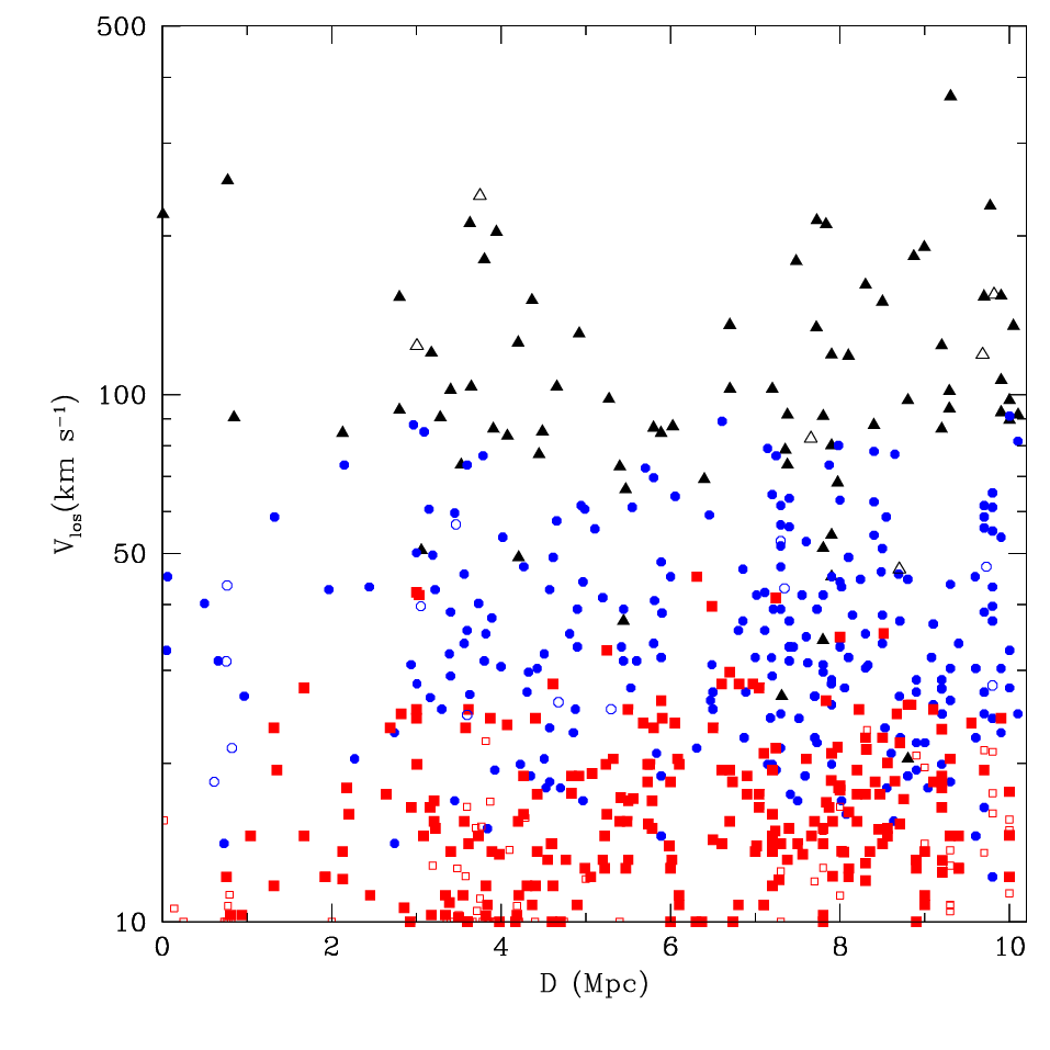
Low accuracy of the for some small galaxies force us to use the distribution of the line-widths not corrected for the inclination. In this respect we follow the suggestion of Papastergis et al. (2011), and use line-widths as the main characteristics of observed galaxies. In order to simplify the comparison with the theory, instead of the full width we use half-width as a proxy for the projected circular velocity.
Figure 2 presents the distribution of line-widths for galaxies in the Local Volume. The overall increase of the number of galaxies at large distances is simply the reflection of increasing volume. However, there is a real drop in the number-density of galaxies at distance Mpc, which is followed by an enhancement at Mpc due to large galaxy groups at that distance. Another effect is a gradual increase in the number of early-type galaxies for low-luminosity galaxies. Incompleteness of the sample manifests itself as the apparent lack of galaxies with at Mpc.
There are two ways of comparing the observational results of the distribution of line-width with the theory: (1) One can apply corrections to the theoretical predictions as was suggested by Papastergis et al. (2011). This is done separately for disk galaxies and for early-type galaxies. For disk galaxies we assume a random orientation of disks in space, but no correction is applied for elliptical galaxies, for which we assume . (2) One can also de-project the observational sample by assuming a random orientation of disk galaxies. This can be done in a number of ways, here we use a parametric fitting. We use an analytical function of the distribution of the circular velocities with free parameters, then parameters are tuned to reproduce the observed distribution of line-width.

Because neutral hydrogen typically extends well beyond the optical radius even for dwarf galaxies (Côté et al., 2000; Swaters et al., 2002; Begum et al., 2008; Walter et al., 2008; Moiseev, 2014, e.g.,), measurements of HI linewidths using provide estimates of the the rotation velocities at very large distances. To be more specific, they provide the maximum rotational velocity in the region where there is a detectable amount of neutral hydrogen. But is this region large enough? When we compare these velocities with theoretical predictions, we use values of dark matter halos, which also occur at large distances. Therefore, we need to find whether the neutral hydrogen extends far enough to probe .
For most of the galaxies in our sample the extent of the HI component is unknown. Still there are many galaxies for which the measurements exist and we will use two samples of galaxies to shed light on the issue. The first sample is the FIGGS survey (Begum et al., 2008), which, among other parameters provides and the HI radius that corresponds to a column density of atoms per cm-2. We select galaxies that have distance measurements obtained with the Tip of the Red Giant Branch (TRGB) method presented in Rizzi et al. (2007). In Figure 3 open symbols show FIGGS rotational velocities corrected for inclination. In addition we show a compilation of galaxies given by Moiseev (2014) with measured HI extent as filled circles in the same Figure. Similar results were found by Ferrero et al. (2012) and by Papastergis et al. (2014).
The full curves in the plot show circular velocity profiles for dark matter halos with a NFW density distribution and an average concentration. The virial masses for each halo are given in the plot in units of solar mass. Dashed curves show potential correction to values due to the fact that HI is measured only in the central halo region: the correction is less than the indicated value in the plot for all galaxies to the right of a corresponding dashed curve. If we assume that every galaxy has a NFW profile with the average concentration, than there should be a NFW curve passing through every galaxy in the plot. For example, if the galaxy is to the right of a dashed curve with a 15% label, the (with all the corrections to the inclination) gives a with less than 15% error.
In spite of the fact that for some galaxies correction due to the final extent of HI gas may be %, the plot shows that HI typically extends far enough to measure with relatively small error.
2.2 Luminosity Function and Completeness of the sample

The sample of galaxies in the Local Volume was gradually improved and extended over years. Karachentsev et al. (2004, Section 4) discuss completeness of the earlier sample and conclude that within 8 Mpc radius the sample was 70-80 percent complete, implying that about 100 galaxies were missed in that sample. Tikhonov & Klypin (2009) studied completeness of the Local Volume using two methods. They used the updated sample, which had more galaxies, and thus it was nearly complete within 8 Mpc radius for galaxies with . In both methods the ratio of the number of dwarf galaxies to the number of bright galaxies was used as an indicator of completeness since the ratio should not depend on the distance. First, the number of bright galaxies () and the number of dwarf galaxies () inside radial shells of 1 Mpc width were found. If the sample is not complete, we would expect a decline with the distance of the number of dwarf galaxies. The ratio of the number of dwarf to large galaxies did not indicate any decline and confirm the completeness of the sample. Second, galaxies in the zone of avoidance were counted and compared with the counts in the direction of the galactic pole. For the same two subsamples ( and ) Tikhonov & Klypin (2009) found 28 bright galaxies and 18 dwarfs close to the galactic plane (). In the direction of the galactic pole () they found 28 giants and 16 dwarfs. This gives the ratio of dwarfs/bright galaxies equal to 0.64 in the the direction of the galactic pole and 0.57 in the galactic plane. Again, results are compatible with the completeness of the sample used at that time. The present sample is nearly complete to distances Mpc. This almost doubles the volume of the sample as compared with what was used by Tikhonov & Klypin (2009).
Figure 4 shows the luminosity function of galaxies in the Karachentsev et al. (2013) catalog for different subvolumes. Results for the 6 Mpc and 8 Mpc samples were normalized to have the same number-density of galaxies brighter than as in the 10 Mpc sample. There are some variations between different subsamples, but for galaxies brighter than these variations are consistent with pure shot-noise. At smaller luminosities there are clear indications of incompleteness with smaller volumes having more dwarf galaxies with .
For comparison, Figure 4 also presents the luminosity function in the 2dFGRS galaxy catalog (Norberg et al., 2002) and the SDSS sample (Blanton et al., 2005). The 2dFGRS luminosity function was given in magnitudes. We scaled it to the B-magnitudes using the relation (Norberg et al., 2002) and taking . The 2dFGRS luminosity function was estimated only for relatively bright galaxies with . The SDSS luminosity function extends to significantly smaller galaxies with because it was based on a shallow SDSS subsample for galaxies with distances in the range Mpc. We use the double Schechter “corrected” approximation in Table 3 of Blanton et al. (2005) for the g-band magnitudes, which we convert to B-magnitudes using the relation (Blanton & Roweis, 2007) and taking .
The full curve in Figure 4 presents a Schechter fit to the LV data with :
| (2) |
where , , and . Comparison with the SDSS and 2dFGRS luminosity functions indicates that the Local Volume is a typical sample of galaxies for the volume probed. The only systematic deviation which we find is an excess in the Local Volume of very bright galaxies with . Otherwise, it is a normal sample.
We model the incompleteness of the sample at by dividing the measured luminosity function (dotted curve in Figure 4) by the Schechter approximation extrapolated from the brighter galaxies. The ratio of the two gives the selection function of galaxies in the Local Volume. It can be approximated as:
| (3) |
According to these results, the 90 percent completeness is at , which on average corresponds to . We estimate that the sample misses 1/2 of galaxies at and . Motivated by these results, we estimate the selection function in velocities :
| (4) |
We make correction for incompleteness of the catalog by multiplying the observed number of galaxies with given line-width by given by eq. (4). This correction plays a role only for very small galaxies. For example, the correction is only 5 percent for galaxies with , and is totally negligible for larger galaxies.

One may wonder if the surface brightness (SB) completeness could be the cause for the disagreement between the CDM model and observations. The SB completeness of the sample has already been discussed in Karachentsev et al. (2013). Here we reproduce some of the results and arguments of Karachentsev et al. (2013).
Figure 5 shows the average surface brightness within the Holmberg radius of galaxies in the UNGC catalog (see also Figure 6 in Karachentsev et al. (2013)). There is a large spread of SB for a given total absolute magnitude in B band, . There is also a clear trend: less bright galaxies have on average lower SB. The data in the Figure are consistent with a simple assumption that with large spread the surface brightness follows the luminosity. There is an indication that the sample becomes less complete below SB, but it is not clear whether this is a separate limitation of the sample or just a manifestation of incompleteness below .
3 Theoretical predictions for velocity function
There are a number of steps, which we make in this paper in order to predict the distribution of line-widths of galaxies for a cosmological model:
- •
Find the theoretical distribution of circular velocities of dark matter halos. Large cosmological simulations often provide those (Gonzalez et al., 2000; Klypin et al., 2011; Nuza et al., 2013; Schneider et al., 2014, e.g.,). The distribution function must include subhalos. If it does not, it should be corrected.
- •
Correct the dark matter circular velocities for the effect of baryonic infall.
- •
Assuming a random orientation of galactic disks, and, using the observed fraction of early-type galaxies, make a prediction for the distribution of line-widths .
Our predictions rely on a number of assumptions. We assume that maximum of the circular velocity of a dark matter halo measured in cosmological simulations and corrected for baryonic infall gives an estimate of the HI line width. This is a reasonable assumption, if neutral hydrogen extends to large radii where dark matter circular velocity reaches its maxiumum. As Figure 3 shows, this seems to be the case as indicated by those galaxies that have detailed measurements of HI rotation curves. Our procedure also implies that processes related to star formation and stellar feedback do not change the total mass of galaxies (including the dark matter mass) inside the radius of HI extent (typically times the optical radius of galaxies). More detaled discussion of these effects is presented in Section 6.
We use the MultiDark suit of simulations (Klypin et al., 2014) to construct the velocity function in the CDM model. Specifically, we use the Bolshoi (Klypin et al., 2011) and MultiDark Prada et al. (2012) simulations for WMAP7 cosmological parameters. The the Planck cosmology we use BolshoiP and MDPL simulations (Klypin et al., 2014). These simulations are done with the ART and Gadget codes.
Halos in the simulations were identified with the Bound Density Maximum (BDM) spherical overdensity code (Riebe et al., 2013). For each halo or subhalo the halofinder provides the maximum circular velocity . In the following instead of we use notation and call it the circular velocity.
The Bolshoi and BolshoiP simulations are complete for halos and subhalos down to (Klypin et al., 2011). Multidark and MDPL simulations are complete down to (Klypin et al., 2013). Results of the simulations for halos and subhalos are presented in Figure 6. At small the circular velocity function is very close to a power-law. This power-law behaviour of the velocity function is consistent with the results of much high resolution simulations of individual halos and small regions (Diemand et al., 2008; Klypin et al., 2011; Sawala et al., 2014, e.g.,). It allows us to extrapolate our results to smaller values of .
We use the following approximations for the differential circular velocity functions for halos and subhalos in the range :
| (5) |
where the normalization is equal to
| (6) |

We use also predictions of the velocity function for the Warm Dark Matter models made by Schneider et al. (2014) for models with thermal neutrino masses KeV. The velocity function was derived from halo mass function (Schneider et al., 2013) and halo concentration-mass dependence (Schneider et al., 2012). The WDM mass functions were estimated for the WMAP7 cosmology using -body simulations, and were approximated with analytical models. These estimates are done only for distinct halos, and thus they do not include subhalos. The fraction of satellites for given circular velocity is relatively small. We account for the missing subhalos in the Schneider et al. (2014) data by multiplying the abundance of distinct halos by factor 1.25, which is the same fraction of subhalos as in the CDM model for circular velocities . This is a good approximation for circular velocities above , because the effects of WDM are relatively small for these velocities and for neutrino masses considered here (KeV). For smaller velocities this likely overestimates the effect, however there must be a significant number of small satellites to explain dwarf satellites in the Local Group and in the Local Volume. So, our estimate of the fraction of subhalos in the WDM models seems to be reasonable.


In practice we use an analytical approximation to the data provided by Schneider et al. (2014). The following analytical form provides a 2% accurate fit the data on the WDM circular velocity function corrected for the subhalos abundance:
| (7) |
where the WDM suppression factor is
| (8) | |||||
Here the WDM mass is given in the units of 1 KeV. Figure 6 presents results for velocity function in the WDM models. We note that the WDM velocity function has a simple dependence on mass : the suppression factor in eqs. (7-8) depends only on the product . This is likely related to the fact that the CDM velocity function for the relevant velocity range is nearly a power-law, and, thus, it is scale-free. The only scale dependence comes from the power spectrum suppression due to .
This simple scaling relation of the WDM models allows one to estimate the WDM predictions for any and for different cosmological parameters. When comparing with observations, we re-scale the abundance of halos in the WDM models to the Planck cosmological parameters using eqs. (5-6) for and the suppression factor given by eq. (8).
Detailed analysis of the effects of baryons on the circular velocity function was done by Trujillo-Gomez et al. (2011) and Dutton et al. (2011). The impact of baryons is small for galaxies hosted by halos with . More massive galaxies are more affected. For example, modeling of the Milky Way galaxy Klypin et al. (2002), which used the CDM predictions (the NFW profile with realistic concentration and spin parameter), indicates that the dark-matter-only maximum of the circular velocity should be . Taking for circular velocity of the Milky Way, we find that the baryons increase the circular velocity by a factor . In this paper we approximate the complex effects of baryons studied by Trujillo-Gomez et al. (2011) using a simple fitting function of the results presented in Figure 12 of Trujillo-Gomez et al. (2011) 11 1 Unlike Trujillo-Gomez et al. (2011), who estimate circular velocities at radius of 10 kpc, we always use the the maximum circular velocity . Specifically, we use the following fit:
| (9) | |||||
| (10) |
where is maximum of circular velocity for dark-matter-only predictions, and is the the circular velocity corrected for the effect of baryons.
4 How typical is the Local Volume: theoretical view
The Local Volume has many hundreds of galaxies, and, thus one expects that to some degree it is a representative sample of galaxies inside a Mpc sphere selected not to be centered on a void or a cluster of galaxies. Indeed, the B-band luminosity function presented in Figure 4 is consistent with this expectation: the luminosity function in the Local Volume is close to the luminosity function in the SDSS catalog for an overlapping range of magnitudes. How can this be considering that the size of the Local Volume is relatively small?
One needs to keep in mind that the Local Volume is not a randomly selected sphere of 10 Mpc centered on a Milky-Way type galaxy. If it were, the region would have been a factor of overdense (Hogg et al., 2005; Zehavi et al., 2011, e.g.,) reflecting a large amplitude of the galaxy-galaxy correlation function on a few Megaparsec scale. It also would have had a very large level of fluctuations because of cosmic variance: occasionally it would fall on either a cluster of galaxies or a nearly empty void. One property of the Local Volume makes it more representative of the average Universe, and makes the density inside the 10 Mpc sphere close to the average density in the Universe. This is the fact that the Local Volume does not have large groups or clusters inside its boundaries.
We can measure the magnitude of fluctuations and test the effects of different selection conditions by studying properties of analogs of the Local Volume in numerical simulations of the CDM model. For this purpose we use the BolshoiP simulation. As a center of a Local Volume candidate we chose a distinct halo in the mass range . We then select only those candidates that have a number of large halos and subhalos with the maximum circular velocity larger than within a radius of . This number of large halos is compatible with the number of large galaxies observed in the Local Volume (see, for example, Figure 2). We use halos and subhalos with maximum circular velocity larger than without any corrections for baryons.


The average number-density profile and the average radial velocity of (sub)halos in the Local Volume candidates are shown in Figures 7 and 8. As one may have expected, there are substantial overdensities and, consequently large deviations from the Hubble flow for scales below . This is just the reflection of the fact that the sample is centered on a large halo and that halos highly correlate on small scales. However, the Local Volume candidates have dramatically smaller deviations on larger scales, which is a reflection of the selection condition; just as the real Local Volume, these candidates are not allowed to have large groups or clusters inside their boundaries.
Figure 9 shows the velocity functions for the Local Volume candidates inside spheres of radius as well as for two other unconstrained samples. On average, the Local Volume candidates show little systematic deviations from the velocity function of the whole simulation. The rms fluctuations are larger than the Poissonian estimates, but they are still reasonably small.


5 Results: Velocity function of galaxies
The left panel in Figure 10 shows estimates of the galaxy velocity function in the Local Volume for different subsamples. The number-density in each subsample is not the same mostly because of a large excess of bright galaxies at 3.5-4 Mpc distance from the Milky Way. Effect of the fluctuation declines with the volume, and for the 10 Mpc sample the number-density is close to the average number-density in the much larger SDSS sample, as indicated in Figure 4. For this reason estimates of the abundance of galaxies in the 6 and 8 Mpc samples were normalized to have the same number-density of galaxies brighter than as in the 10 Mpc sample. Once normalized to the same number-density, comparison of different subsample serves as indicator of stability of estimates of the velocity function.
The full curve in the plot shows a fit to the 10 Mpc data:
| (11) |
Errors of this approximation are dominated by the cosmic varience, which was discussed in Section 4 and presented in figure 9. The errors are for circular velocities .
In the right panel of Figure 10 we compare our estimates with the HIPASS (Zwaan et al., 2010) and ALFALFA (Papastergis et al., 2011) results. Our estimates are systematically larger because HIPASS and ALFAFA do not include gas poor early-type galaxies while those galaxies are included in the Local Volume sample. However, the fraction of the early-type galaxies is relatively small, as indicated in the top panel in Figure 4. So, the agreement between different catalogs is reasonably good for velocities in the range . At smaller velocities the Local Volume results are substantially above HIPASS and ALFALFA mostly because the fraction of gas-poor galaxies increases and likely because of incompleteness in the HIPASS data.
We compare our results with theoretical predictions in Figure 11. In the left panel we confront observational results with the predictions of the CDM model with the Planck parameters. Correction for baryon infall becomes progressively more important for . Thanks to this correction, the CDM model makes a reasonably accurate account for the abundance of bright galaxies. At smaller velocities effects of baryons are not significant. Here the theory clearly has substantial problems.
However, the real problem for the model is the abundance of relatively large dwarf galaxies with . The CDM model overpredicts the abundance of those galaxies by a factor of 3.5-7.5 for the model with the Planck parameters. These galaxies are hardly affected by possible effects of reionization and cannot be stopped from forming stars by few supernovae. These galaxies are relatively bright with . For these luminosities the Local Volume catalog is nearly complete. We definitely can exclude the possibility that of these galaxies are missed. In short, it is difficult to reconcile the CDM predictions with observations.
The WDM models are somewhat better. In the right panel of Figure 11 we test the WDM models. Models with KeV can be excluded because they do not provide enough reduction of the number of dwarf galaxies. Smaller masses help to suppress the low-mass tail of the velocity function, but the shape of is not right. For example, the model with KeV is still above data points with , and it misses the smaller ’s. Further decreasing would improve points with but ruin .
The circular velocity function of observed galaxies can be reconstructed in a statistical sense by following the same steps, which we do when we make the transition from theoretical circular velocity function to the distribution of line-width . In the case of observations we assume an analytical function with free parameters. For each set of the parameters we make a prediction for by assuming a random orientation of disk galaxies and by taking the observed fraction of early type galaxies. We then change the free parameters until we get an acceptable fit to the data. The best fit to observed circular velocity function of galaxies is:
| (12) | |||||
Note that the slope of the circular velocity function is close, but slightly smaller that the slope of the related line-width function . One can show analytically that a pure power-law gives a power-law line-width function with exactly the same slope. The small change in the slope between and seen in Figure 12 is, thus, due to the bending of at large .
Comparison of the observed and theoretical circular velocity functions presented in Figure 12 leads to the same conclusion, which we found comparing the line-width functions in Figure 11: the CDM model gives a good fit for massive galaxies with , but it has problems explaining the abundance of galaxies with small velocities. However, the disagreement is slightly worse for functions as compared with . For example, at the disagreement with the CDM-Planck model was factor 3.5 for the line-width functions. It is factor of 6 for the circular velocities. Qualitatively, it is clear why the disagreement is worse in -space: some fraction of galaxies with given are intrinsically larger galaxies with large , for with the CDM predicts correct abundance.
6 Discussion

Estimates of the abundance of galaxies with a given line-width presented in Figure 10 for different observational samples shows that results mostly agree for intermediate-size galaxies with . The Local Volume results are systematically above the HIPASS (Zwaan et al., 2010) and ALFALFA (Papastergis et al., 2011) estimates, but this is mostly due to the fact that HI measurements do not cover early-type galaxies, which are present in the Local Volume. The agreement between the ALFALFA (Papastergis et al., 2011) and Local Volume results is particular good once ALFALFA results are corrected by the fraction of early-type galaxies in the Local Volume as presented in Figure 4. This is very encouraging because it indicates that we finally have an accurate measurement of the abundance of galaxies in a broad range of velocities .

Figure 13 compares observational estimates for the circular velocity function of galaxies with theoretical predictions for the CDM and WDM models. As one may have expected, the CDM model dramatically overpredicts the abundance of dwarf galaxies. The WDM is not better. It was designed to fix the small-scale problems of the CDM. As far as the abundance of dwarfs is concerned, the WDM still fails.
As Figure 13 shows, the WDM model with KeV predicts a factor too few dwarfs with and a factor of 2 too many at . As plots in Figure 11 indicate, decreasing neutrino mass to KeV fixes the problem with , but it also ruins the small-scale tail by reducing the abundance of dwarfs by another factor of 2. Thus, there seem to be no neutrino mass that produces an acceptable fit to the data.
Additional limitations on the WDM model are coming from the clustering observed in the Lyman- forest (Seljak et al., 2006; Viel et al., 2008; Viel et al., 2013, e.g.,). Recent results of Viel et al. (2013) constrain the (thermal) neutrino mass KeV at level. Our results indicate that neutrino mass above 2 KeV is incompatible with the observed abundance of field dwarf galaxies in the Local Volume. Our conclusions regrading the inability of WDM models to explain the observational data are in agreement with those of Schneider et al. (2014).
In spite of the fact that our estimates of the abundance of field galaxies are above the previous estimates, the CDM predictions for the velocity function are still well above the observations. This is neither new (Tikhonov & Klypin, 2009; Trujillo-Gomez et al., 2011; Schneider et al., 2014) nor surprising. The overabundance of satellites (Klypin et al., 1999; Moore et al., 1999) in the CDM model is a well established problem, and it has the same origin as the overabundance of field galaxies. However, the galaxy velocity function rises the problem to a different level.
It is interesting to compare the overabundance of satellites in the Local Group with the overabundance of field galaxies:
Most of the galaxies in the Local Volume are not satellites (though there are some). Thus, the problem with the field galaxies cannot be solved by appealing to effects such as the tidal forces and ram pressure stripping due to the central “parent”. For satellites close to their parent (say, distances less than virial radius) the stripping and tides are a possible solution (Zolotov et al., 2012; Arraki et al., 2014) for the problems with structural properties of the largest dwarf spheroidal galaxies – the “too big to fail” problem (Boylan-Kolchin et al., 2011).
However, these processes are not expected to be efficient enough for satellites in the outskirts (kpc) of the Local Group. Indeed, Garrison-Kimmel et al. (2014) find an excess of theoretically predicted large () satellites. This situation is similar to the problem of the abundance of field dwarf galaxies, which we find in this paper.
The main problem in the Local Group was related with dwarf spheroidal galaxies. In the Local Volume most of “problematic” galaxies are dwarf irregular galaxies, which are star-forming gas-reach galaxies.
The satellite problem starts at relatively small galaxies with and . There is practically no issue with the number of satellites with : the theory predicts as many as observed (Klypin et al., 1999; Kravtsov, 2010, e.g.,). The situation is much worse in the field, where the disagreement is already very severe for galaxies with and virial masses . This can be expressed in a number of ways. At the ratio of of the predicted (eq. (5)) to the observed (eq. (12)) number of galaxies is 6 for the Planck cosmology. The total number of galaxies in the Local Volume (distances Mpc) with circular velocities in the range is , while the theory predicts .
What can possibly be a solution for the field problem?
Observations: It is possible and very likely that a number of small dwarfs galaxies with were missed. However, at the disagreement with the theory is a factor of 20. In order to reconcile observations with the CDM model, most of the dwarfs must have been missed in the Local Volume sample: an unlikely proposition considering the convergence of results on the luminosity function at .
The main problem is with larger galaxies in the range of velocities . These galaxies are bright, , and it is unrealistic to assume that the Local Volume sample missed 1000 of them. The only remote possibility is that a large fraction of the galaxies are low surface brightness dwarf spheroidal galaxies with surface brightness well below 25 mag per square arcsecond. So far, none of these bright and extra low surface brightness galaxies have been found.
Theory: It is difficult to resolve the overabundance of field galaxies because some of the problematic galaxies are relatively large with and . For example, photoheating during reionization hardly can affect these objects. Another possible way out is not to have the star formation in most of these galaxies. However, this does not help either because these objects would keep their neutral hydrogen, and thus would be observed as HI clouds without stellar light. However, those massive dark HI clouds have not been found. Mass of the clouds should be , if they follow the Baryonic Tully-Fisher relation.
One may think that flattening of the dark matter cusp in dwarf galaxies in numerous episods of contraction and expansion due to centrally concentrated bursts of star formation (Mashchenko et al., 2006; Pontzen & Governato, 2012, e.g.,) may solve the problem with the abundance of field dwarfs. Indeed, large variations in the gravitational potential of a forming dwarf galaxy are capable of reducing the dark matter density in the central galaxy region, which in turn reduces the circular velocity (Governato et al., 2010; Teyssier et al., 2013; Di Cintio et al., 2014; Madau et al., 2014). Unfortunately, this reduction in the central dark matter density does not automatically resolve the issue.
The dark matter, which was heated and pushed from the cusp, does not leave the galaxy. It just moves away from the central cusp and settles at somewhat larger radius (Teyssier et al., 2013; Madau et al., 2014). Within this radius the total mass does not change, and thus the circular velocity does not change either. The question is how large is the radius and how does it compare to the radius that defines the observed HI line width.
Rotation curves in dwarf galaxies are rising even at large radii. Thus, it is the outskirts of galaxies that define the observed HI line width (Oh et al., 2008; Moiseev, 2014, e.g.,). The problem is that the neutral hydrogen in galaxies extends to very large radii: substantially larger than the optical radius, where thrashing and heating of the dark matter happens. For example, data in Figure 3 indicates that gas in galaxies with rotational velocity extends to 2–4 kpc. (See also Figure 3 in Ferrero et al. (2012) and Figures 5 and B.1 in Papastergis et al. (2014) for simular results). Hydrodynamical simulations show that the size of the core in such galaxies should be (Teyssier et al., 2013; Di Cintio et al., 2014; Madau et al., 2014), which is not enough to substantially reduce HI line width at . The problem is even worse for smaller galaxies with rotational velocity and virial mass . Current numerical simulations of these galaxies (Di Cintio et al., 2014; Madau et al., 2014) indicate that there is not enough energy in the stellar feedback to flatten dark matter cores of these dwarfs.
It is possible that current simulations may not implemented all effects of the stellar feedback, and that better models will show larger decline in the density. Another possible solution for the overabundance problem is the possibility that in reality there are many missed very low surface brightness galaxies with just enough star formation to keep the gas ionized. So, the galaxies are not detected in both HI and optical observations.
After our paper was submitted for publication, Papastergis et al. (2014) came to similar conclusions the regarding the extend of the HI gas in dwarf galaxies: neutral gas extends far enough to probe the part of the circular velocity curve that defines value of . They also confirm our findings on the disagreement between observations and theory on the abundance of galaxies with given circular velocities.
7 Conclusions
The abundance of galaxies as a function of their circular velocity is a fundamental statistics, which provides a sensitive probe for theoretical predictions (Cole & Kaiser, 1989; Shimasaku, 1993; Gonzalez et al., 2000; Zavala et al., 2009; Trujillo-Gomez et al., 2011; Schneider et al., 2014). Because it is difficult to measure the velocity function, only recently observations became capable of producing reasonably converging estimates of for different samples (Zwaan et al., 2010; Papastergis et al., 2011). Abundance of galaxies with given circular velocity or line-width in the Local Volume (distances less than 10 Mpc) provide a valuable information that can be difficult to obtain using other samples (Karachentsev et al., 2004; Karachentsev et al., 2013) because in the Local Volume we observe small galaxies, and the sample has galaxies of all morphological types.
We find that the observed velocity function of galaxies of all morphological types has a shallow slope at small velocities and a relatively steep decline at large velocities. Equations (11) and (12) give approximations for the observed line-width and for the reconstructed 3D circular velocity functions .
Results for in the Local Volume are consistent with the velocity function in the much larger HI-based ALFALFA sample (Papastergis et al., 2011) once the latter is corrected for the fraction of early-type galaxies not detected in HI observations. This is important because it implies that we now have accurate measurement of the galaxy velocity function for all types of galaxies for circular velocities in the range .
When comparing the Local Volume observational results with theoretical predictions we find that the standard CDM model predicts abundances of intermediate-size galaxies with and corresponding virial masses that are in agreement with the observed abundance of galaxies. However, the shallow slope and the normalization of the velocity function for dwarf galaxies with strongly disagree with the standard CDM model that predicts the slope for dark matter halos and subhalos found in body cosmological simulations. The Warm Dark Matter (WDM) models cannot explain the data either, regardless of mass of WDM particle.
The overabundance problem of the field galaxies in many respects is different from the more familiar overabundance of satellite galaxies in the Local Group. Unlike the Local Group, where the problem is in the abundance of gas-poor dSphs with and at small distances , in the field the problem is for gas-rich star-forming galaxies with velocities as large as and on large distances .
Acknowledgments
We are grateful to A. Maccio and A. Schneider for providing us tables with the WDM velocity functions. We thank M. Papastergis for useful discussions and comments. We acknowledge the support of the NSF grants to NMSU, and the support of the grant 14-12-00965 from the Russian Science Foundation. O.N. thanks the non-profit Dmitry Zimin’s Dynasty Foundation for the financial support. The Bolshoi and BolshoiP simulations were run on the Pleiades supercomputer at the NASA Ames Research Center.
References
- Arraki et al. (2014) Arraki, K. S., Klypin, A., More, S., & Trujillo-Gomez, S. 2014, MNRAS, 438, 1466
- Barkana & Loeb (1999) Barkana, R., & Loeb, A. 1999, ApJ, 523, 54
- Begum et al. (2008) Begum, A., Chengalur, J. N., Karachentsev, I. D., Sharina, M. E., & Kaisin, S. S. 2008, MNRAS, 386, 1667
- Bell et al. (2003) Bell, E. F., McIntosh, D. H., Katz, N., & Weinberg, M. D. 2003, ApJ Suppl., 149, 289
- Benson et al. (2003) Benson, A. J., Bower, R. G., Frenk, C. S., et al. 2003, ApJ, 599, 38
- Berlind & Weinberg (2002) Berlind, A. A., & Weinberg, D. H. 2002, ApJ, 575, 587
- Blanton et al. (2005) Blanton, M. R., Lupton, R. H., Schlegel, D. J., et al. 2005, ApJ, 631, 208
- Blanton & Roweis (2007) Blanton, M. R., & Roweis, S. 2007, AJ, 133, 734
- Bode et al. (2001) Bode, P., Ostriker, J. P., & Turok, N. 2001, ApJ, 556, 93
- Boylan-Kolchin et al. (2011) Boylan-Kolchin, M., Bullock, J. S., & Kaplinghat, M. 2011, MNRAS, 415, L40
- Bullock et al. (2001) Bullock, J. S., Kravtsov, A. V., & Weinberg, D. H. 2001, ApJ, 548, 33
- Cappellari et al. (2013) Cappellari, M., Scott, N., Alatalo, K., et al. 2013, MNRAS, 432, 1709
- Chae (2010) Chae, K.-H. 2010, MNRAS, 402, 2031
- Choi et al. (2007) Choi, Y.-Y., Park, C., & Vogeley, M. S. 2007, ApJ, 658, 884
- Colín et al. (2000) Colín, P., Avila-Reese, V., & Valenzuela, O. 2000, ApJ, 542, 622
- Cole & Kaiser (1989) Cole, S., & Kaiser, N. 1989, MNRAS, 237, 1127
- Conroy, Wechsler, & Kravtsov (2006) Conroy C., Wechsler R. H., Kravtsov A. V., 2006, ApJ, 647, 201
- Côté et al. (2000) Côté, S., Carignan, C., & Freeman, K. C. 2000, AJ, 120, 3027
- Dekel & Silk (1986) Dekel, A., & Silk, J. 1986, ApJ, 303, 39
- Di Cintio et al. (2014) Di Cintio, A., Brook, C. B., Macciò, A. V., et al. 2014, MNRAS, 437, 415
- Diemand et al. (2008) Diemand, J., Kuhlen, M., Madau, P., et al. 2008, Nature, 454, 735
- Dutton et al. (2011) Dutton, A. A., Conroy, C., van den Bosch, F. C., et al. 2011, MNRAS, 416, 322
- Ferrero et al. (2012) Ferrero, I., Abadi, M. G., Navarro, J. F., Sales, L. V., & Gurovich, S. 2012, MNRAS, 425, 2817
- Geha et al. (2010) Geha, M., van der Marel, R. P., Guhathakurta, P., et al. 2010, ApJ, 711, 361
- Garrison-Kimmel et al. (2014) Garrison-Kimmel, S., Boylan-Kolchin, M., Bullock, J. S., & Kirby, E. N. 2014, MNRAS, 444, 222
- Gonzalez et al. (2000) Gonzalez, A. H., Williams, K. A., Bullock, J. S., Kolatt, T. S., & Primack, J. R. 2000, ApJ, 528, 145
- Gottloeber & Klypin (2008) Gottloeber, S., & Klypin, A. 2008, in ”High Performance Computing in Science and Engineering Garching/Munich 2007”, Eds. S. Wagner et al, Springer, Berlin 2008 (arXiv:0803.4343)
- Governato et al. (2010) Governato, F., Brook, C., Mayer, L., et al. 2010, Nature, 463, 203
- Guo & White (2014) Guo, Q., & White, S. 2014, MNRAS, 437, 3228
- Hoeft et al. (2006) Hoeft M. et al., MNRAS, 2006, 371, 401
- Hoffman et al. (2007) Hoffman Y., Romano-Díaz E., Shlosman I., Heller C., 2007, ApJ, 671, 1108
- Hogg et al. (2005) Hogg, D. W., Eisenstein, D. J., Blanton, M. R., et al. 2005, ApJ, 624, 54
- Huchra et al. (2012) Huchra, J. P., Macri, L. M., Masters, K. L., et al. 2012, ApJ Suppl., 199, 26
- Kamionkowski & Liddle (2000) Kamionkowski, M., & Liddle, A. R. 2000, Physical Review Letters, 84, 4525
- Karachentsev & Makarov (1996) Karachentsev I.D., Makarov D.I., 1996, AJ, 111, 535
- Karachentsev & Makarov (2001) Karachentsev I.D., Makarov D.I., 2001, Astrofizika, 44, 5
- Karachentsev et al. (2003) Karachentsev I.D. et al., 2003, A&A, 389, 479
- Karachentsev et al. (2004) Karachentsev I.D., Karachentseva V.E., Huchtmeier W.K., Makarov D.I., 2004 AJ, 127, 2031
- Karachentsev (2005) Karachentsev, I. D. 2005, AJ, 129, 178
- Karachentsev et al. (2007) Karachentsev I.D., Karachentseva V., Huchtmeier W., Makarov D., Kaisin S., Sharina M., Mining the Local Volume, 2007, arXiv:0710.0520
- Karachentsev et al. (2013) Karachentsev, I. D., Makarov, D. I., & Kaisina, E. I. 2013, AJ, 145, 101
- Kennedy et al. (2013) Kennedy, R., Frenk, C., Cole, S., & Benson, A. 2013, arXiv:1310.7739
- Kirby et al. (2014) Kirby, E. N., Bullock, J. S., Boylan-Kolchin, M., Kaplinghat, M., & Cohen, J. G. 2014, MNRAS, 439, 1015
- Klypin et al. (1999) Klypin, A., Kravtsov, A. V., Valenzuela, O., & Prada, F. 1999, ApJ, 522, 82
- Klypin et al. (2002) Klypin, A., Zhao, H., & Somerville, R. S. 2002, ApJ, 573, 597
- Klypin et al. (2009) Klypin, A., Valenzuela, O., Colín, P., & Quinn, T. 2009, MNRAS, 398, 1027
- Klypin et al. (2011) Klypin, A. A., Trujillo-Gomez, S., & Primack, J. 2011, ApJ, 740, 102
- Klypin et al. (2013) Klypin, A., Prada, F., Yepes, G., Hess, S., & Gottlober, S. 2013, arXiv:1310.3740
- Klypin et al. (2014) Klypin, A., Yepes, G., Gottlober, S., Prada, F., & Hess, S. 2014, arXiv:1411.4001
- Kraan-Korteweg & Tammann (1979) Kraan-Korteweg, R. C., & Tammann, G. A. 1979, Astronomische Nachrichten, 300, 181
- Kravtsov et al. (1997) Kravtsov, A. V., Klypin, A. A., & Khokhlov, A. M. 1997, ApJ Suppl., 111, 73
- Kravtsov et al. (2004) Kravtsov, A. V., Berlind, A. A., Wechsler, R. H., et al. 2004, ApJ, 609, 35
- Kravtsov (2010) Kravtsov, A. 2010, Advances in Astronomy, 2010
- Mac Low & Ferrara (1999) Mac Low, M.-M., & Ferrara, A. 1999, ApJ, 513, 142
- Madau et al. (2014) Madau, P., Shen, S., & Governato, F. 2014, ApJLett, 789, LL17
- Makarov & Karachentsev (2011) Makarov, D., & Karachentsev, I. 2011, MNRAS, 412, 2498
- Mashchenko et al. (2006) Mashchenko, S., Couchman, H. M. P., & Wadsley, J. 2006, Nature, 442, 539
- Mo et al. (1998) Mo, H. J., Mao, S., & White, S. D. M. 1998, MNRAS, 295, 319
- Moiseev (2014) Moiseev, A. V. 2014, Astrophysical Bulletin, 69, 1
- Montero-Dorta & Prada (2009) Montero-Dorta, A. D., & Prada, F. 2009, MNRAS, 399, 1106
- Moore et al. (1999) Moore, B., Ghigna, S., Governato, F., et al. 1999, ApJLett, 524, L19
- Navarro, Frenk, & White (1997) Navarro J. F., Frenk C. S., White S. D. M., 1997, ApJ, 490, 493
- Norberg et al. (2002) Norberg, P., Cole, S., Baugh, C. M., et al. 2002, MNRAS, 336, 907
- Nuza et al. (2013) Nuza, S. E., Sánchez, A. G., Prada, F., et al. 2013, MNRAS, 432, 743
- Oh et al. (2008) Oh, S.-H., de Blok, W. J. G., Walter, F., Brinks, E., & Kennicutt, R. C., Jr. 2008, AJ, 136, 2761
- Papastergis et al. (2011) Papastergis, E., Martin, A. M., Giovanelli, R., & Haynes, M. P. 2011, arXiv:1106.0710
- Papastergis et al. (2014) Papastergis, E., Giovanelli, R., Haynes, M. P., & Shankar, F. 2014, arXiv:1407.4665
- Polisensky & Ricotti (2014) Polisensky, E., & Ricotti, M. 2014, MNRAS, 437, 2922
- Pontzen & Governato (2012) Pontzen, A., & Governato, F. 2012, MNRAS, 421, 3464
- Prada et al. (2012) Prada, F., Klypin, A. A., Cuesta, A. J., Betancort-Rijo, J. E., & Primack, J. 2012, MNRAS, 423, 3018
- Reed et al. (2007) Reed D. S., Bower R., Frenk C. S., Jenkins A., Theuns T., 2007, MNRAS, 374, 2
- Riebe et al. (2013) Riebe, K., Partl, A. M., Enke, H., et al. 2013, Astronomische Nachrichten, 334, 691
- Rizzi et al. (2007) Rizzi, L., Tully, R. B., Makarov, D., et al. 2007, ApJ, 661, 815
- Sawala et al. (2014) Sawala, T., Frenk, C. S., Fattahi, A., et al. 2014, arXiv:1412.2748
- Seljak et al. (2006) Seljak, U., Makarov, A., McDonald, P., & Trac, H. 2006, Physical Review Letters, 97, 191303
- Sheth & Tormen (2002) Sheth R. K., Tormen G., 2002, MNRAS, 329, 61
- Schneider et al. (2012) Schneider, A., Smith, R. E., Macciò, A. V., & Moore, B. 2012, MNRAS, 424, 684
- Schneider et al. (2013) Schneider, A., Smith, R. E., & Reed, D. 2013, MNRAS, 433, 1573
- Schneider et al. (2014) Schneider, A., Anderhalden, D., Macciò, A. V., & Diemand, J. 2014, MNRAS, L51
- Schultz et al. (2014) Schultz, C., Oñorbe, J., Abazajian, K. N., & Bullock, J. S. 2014, arXiv:1401.3769
- Shapiro et al. (2004) Shapiro, P. R., Iliev, I. T., & Raga, A. C. 2004, MNRAS, 348, 753
- Sheth et al. (2003) Sheth, R. K., Bernardi, M., Schechter, P. L., et al. 2003, ApJ, 594, 225
- Shimasaku (1993) Shimasaku, K. 1993, ApJ, 413, 59
- Somerville & Primack (1999) Somerville, R. S., & Primack, J. R. 1999, MNRAS, 310, 1087
- Somerville et al. (2012) Somerville, R. S., Gilmore, R. C., Primack, J. R., & Domínguez, A. 2012, MNRAS, 423, 1992
- Strigari et al. (2008) Strigari, L. E., Bullock, J. S., Kaplinghat, M., et al. 2008, Nature, 454, 1096
- Swaters et al. (2002) Swaters, R. A., van Albada, T. S., van der Hulst, J. M., & Sancisi, R. 2002, Astron.& Astrophys., 390, 829
- Teyssier et al. (2013) Teyssier, R., Pontzen, A., Dubois, Y., & Read, J. I. 2013, MNRAS, 429, 3068
- Tikhonov & Klypin (2009) Tikhonov, A. V., & Klypin, A. 2009, MNRAS, 395, 1915
- Tinker et al. (2008) Tinker J., Kravtsov A. V., Klypin A., Abazajian K., Warren M., Yepes G., Gottlöber S., Holz D. E., 2008, ApJ, 688, 709
- Trujillo-Gomez et al. (2011) Trujillo-Gomez, S., Klypin, A., Primack, J., & Romanowsky, A. J. 2011, ApJ, 742, 16
- Viel et al. (2008) Viel, M., Becker, G. D., Bolton, J. S., et al. 2008, Physical Review Letters, 100, 041304
- Viel et al. (2013) Viel, M., Becker, G. D., Bolton, J. S., & Haehnelt, M. G. 2013, PhysRevD, 88, 043502
- Walter et al. (2008) Walter, F., Brinks, E., de Blok, W. J. G., et al. 2008, AJ, 136, 2563
- Warren et al. (2006) Warren M. S., Abazajian K., Holz D. E., Teodoro L., 2006, ApJ, 646, 881
- White & Frenk (1991) White, S. D. M., & Frenk, C. S. 1991, ApJ, 379, 52 ¡
- Zavala et al. (2009) Zavala, J., Jing, Y. P., Faltenbacher, A., et al. 2009, ApJ, 700, 1779
- Zehavi et al. (2011) Zehavi, I., Zheng, Z., Weinberg, D. H., et al. 2011, ApJ, 736, 59
- Zentner et al. (2005) Zentner, A. R., Berlind, A. A., Bullock, J. S., Kravtsov, A. V., & Wechsler, R. H. 2005, ApJ, 624, 505
- Zolotov et al. (2012) Zolotov, A., Brooks, A. M., Willman, B., et al. 2012, ApJ, 761, 71
- Zwaan et al. (2010) Zwaan, M. A., Meyer, M. J., & Staveley-Smith, L. 2010, MNRAS, 403, 1969