Network Controllability Is Determined by the Density of Low In-Degree
and Out-Degree Nodes
Abstract
The problem of controllability of the dynamical state of a network is central in network theory and has wide applications ranging from network medicine to financial markets. The driver nodes of the network are the nodes that can bring the network to the desired dynamical state if an external signal is applied to them. Using the framework of structural controllability, here we show that the density of nodes with in-degree and out-degree equal to , and determines the number of driver nodes of random networks. Moreover we show that networks with minimum in-degree and out-degree greater than 2, are always fully controllable by an infinitesimal fraction of driver nodes, regardless on the other properties of the degree distribution. Finally, based on these results, we propose an algorithm to improve the controllability of networks.
pacs
89.75.Fb, 64.60.aq, 05.70.FhThe controllability of a network [1, 2, 3, 4, 5, 6, 7, 8, 9, 10] is a fundamental problem with wide applications ranging from medicine and drug discovery [11], to the characterization of dynamical processes in the brain [12, 13, 14], or the evaluation of risk in financial markets [15]. While the interplay between the structure of the network [16, 17, 18, 19] and the dynamical processes defined on them has been an active subject of complex network research for more than ten years [20, 21], only recently the rich interplay between the controllability of a network and its structure has started to be investigated. A pivotal role in this respect has been played by a paper by Liu et al. [6], in which the problem of finding the minimal set of driver nodes necessary to control a network was mapped into a maximum matching problem. Using a well established statistical mechanics approach [24, 25, 26, 27, 22, 23], Liu et al. [6] characterize in detail the set of driver nodes for real networks and for ensembles of networks with given in-degree and out-degree distribution. By analyzing scale-free networks with minimum in-degree and minimum out-degree equal to 1 they have found that the smaller is the power-law exponent of the degree distribution, the larger is the fraction of driver nodes in the network. This result has prompted the authors of [6] to say that the higher is the heterogeneity of the degree distribution, the less controllable is the network. Later, different papers have addressed questions related to controllability of networks with similar tools [7, 28].
In this Letter we consider the network controllability and its mapping to the maximum matching problem, exploring the role of low in-degree and low out-degree nodes in the network. We show that by changing the fraction of nodes with in-degree and out-degree less than 3, the number of driver nodes of a network can change in a dramatic way. In particular if the minimum in-degree and the minimum out-degree of a network are both greater than 2 then any network, independently on the level of heterogeneity of the degree distribution, is fully controllable by an infinitesimal fraction of nodes. Therefore we show that the heterogeneity of the network is not the only element determining the number of driver nodes in the network and that this number is very sensible on the fraction of low in-degree low out-degree nodes of the network. This result allows us to propose a method to improve the controllability of networks by decreasing the density of nodes with in-degree and out-degree less than , adding links to the network.
The structural controllability of a network. Given a graph of nodes, we consider a continuous-time linear dynamical system
| (1) |
in which the vector , of elements with , represents the dynamical state of the network, is (asymmetric) matrix describing the directed weighted interactions within the network, and is a matrix describing the interaction between the nodes of the graph and external signals, indicated by the vector of elements and . For any given realization of and , the dynamical system is controllable if it satisfies Kalman’s controllability rank condition, i.e. the matrix is full rank. In addition to the fact that the verification of Kalman’s condition can be computationally very demanding for large systems, in most real systems the notion of exact controllability is unusable since the entries of and are not perfectly known. As an alternative, if we assume that the non-zero matrix elements of and are free parameters, we can consider the concept of structural controllability [5]. The system is structurally controllable if for any choice of the free parameters in and , except for a variety of zero Lebesgue measure in the parameter space, is full rank [5]. Since structural controllability only distinguishes between zero and non-zero entries of the matrices and , a given directed network is structurally controllable if it is possible to determine the input nodes (i.e. the position of the non-zero entries of the matrix ) in a way to control the dynamics described by any realization of the matrix with the same non-zero elements, except for atypical realizations of zero measure. In practice, a network can be structurally controlled by identifying a minimum number of driver nodes, that are controlled nodes which do not share input vertices. In their seminal paper [6], Liu and coworkers showed that this control theoretic problem can be reduced to a well-known optimization problem: their Minimum Input Theorem states that the minimum set of driver nodes that guarantees the full structural controllability of a network is the set of unmatched nodes in a maximum matching of the same directed network.
The maximum matching problem. A matching of a directed graph is a set of directed edges without common start or end vertices, and it is maximum when it contains the maximum possible number of edges. The problem of finding a maximum matching of a directed graph can be cast on a statistical mechanics problem, by introducing variables on each directed link from node to node , indicating whether the directed link is in () or not (). The configurations of variables have to satisfy the following matching condition,
| (2) |
where indicates the set of nodes that point to node in the directed network, and indicates the set of nodes that are pointed by node . Moreover the variables should minimize the energy function
| (3) |
Note that a vertex is matched if it is the endpoint of one of the edges in the matching, otherwise the vertex is unmatched. It follows that , where is the number of unmatched nodes in the network, and this number also determines the minimum number of driver nodes required to fully control the network. Following Refs.[22, 6], we use the cavity method in the zero-temperature limit, to study the statistical properties of maximum matchings on directed random graphs for which the locally-tree-like approximation holds. Under the decorrelation (replica-symmetric) assumption, the energy of a maximum matching can be written in terms of the cavity fields (or messages) or sent from a node to the linked node . The fields are sent in the same direction or in the opposite direction of the links and indicate the following messages [22]: indicates match me, indicates do not match me, finally indicates do what you want. In fact the energy follows (see Supplemental Material (SM) [31] for details)
| (4) | |||||
in which for each directed link the cavity fields satisfy the following zero-temperature version of the Belief Propagation (BP) equations, also known as Max-Sum (MS) equations,
| (5a) | |||||
| (5b) | |||||
with the assumption that the maximum over an empty set is equal to .
In the infinite size limit, the MS equations are closed for cavity fields with support on [22, 6, 23]. These equation can be solved by iteration using the BP/MS algorithm.
Sufficient condition for the full controllability of networks.
Let us now show that for any network topology if the in-degree and the out-degree of the network is greater than 2 the fraction of driver nodes is zero. First we observe that the configuration in which all fields are zero , i.e. , is an allowed solution of the Eqs. as soon as the minimum in-degree and minimum out-degree equal to 1. In fact if a node has in-degree 1 this link must be matched, and a similar situation occurs for the nodes with out-degree 1, generating a set of hard constraints incompatible with the configuration in which all the fields are zero, while if the minimum in-degree or out-degree of the network is greater than 1, all the nodes can be matched in a variety of ways therefore all the fields can be equal to zero. This solution corresponds to a fraction of driver nodes if the minimum in-degree and the minimum out-degree are greater than 1. This solution is also stable if, when we change a single field from zero to a value different from zero, the perturbation does not propagate in the network. Suppose that is changed, say, from to , meaning that the message is match me, then all the nodes neighbor of and different from receive a message do not match me. But if all the nodes have more than 2 incoming links, also if the link is not matched they can still send to their incoming neighbors the messages do what you want since there are different ways in which the matching can be achieved and they do not have to impose to any of their other links to be matched. Therefore the perturbation does not propagate in the network.
A similar argument holds for a change of the field to 1 which does not propagate if the out-degree of the network is greater than 2. This stability argument shows that for every tree-like network for which the BP/MS equations are valid, if the in-degree and the out-degree of the network is greater than 2 then the density of driver nodes is . Note that this a sufficient condition for the stability of the solution but more stringent conditions are discussed in the following for networks with given degree distribution.

and Out-Degree Nodes) and (left), (right). The density is obtained by numerically solving the BP/MS equations for an ensemble of networks with given degree distribution. The region in which is non-physical.
Conditions for the full controllability of random networks. In the following we focus on ensembles of random networks with given in-degree and out-degree distribution and . In this case (see SM [31]), it is possible to write the BP/MS equations and the energy in terms of the probabilities and with that the cavity fields and are respectively given by .

From the BP/MS equations of the matching problem on random networks with given degree distribution, we found that the solution is allowed if and only if . The replica-symmetric cavity equations are supposed to give the correct solution to the maximum matching problem if no instabilities take place. By analysing the stability condition of the BP/MS equations [31], we find that the stability conditions for this solution in an ensemble of networks with given in-degree and out-degree sequence, are
| (6) |
In particular when the minimum in-degree and the minimum out-degree of scale-free networks are both greater than , i.e. , the fraction of driver nodes is zero in the thermodynamic limit, for any choice of the degree distribution with this property. By changing the minimum in-degree and minimum out-degree of the network the number of driver nodes can change dramatically, independently of the tail of the degree distribution and the level of degree heterogeneity.
In order to use the above calculation to estimate the role of low-degree nodes on the fate of the zero-energy solution in finite networks, we consider uncorrelated random graphs with the following power-law degree distribution
with a constant determined by normalization and maximum degree for and for , that is the minimum between the structural cutoff [29, 30] of the network and the natural cutoff of the degree distribution. These networks can be generated numerically using the configuration model. As long as , the density of driver nodes goes to zero () for any exponent . More generally, the density of driver nodes changes dramatically as a function of and as shown by the heat map in Fig. 1 for . Moreover, in Fig. 2, we plot the phase diagram for indicating the region where the solution is stable both for a finite network of nodes (white solid line) and for (white dotted line). Note that, for , stability line converges quite slowly to zero in the infinite size limit.

and Out-Degree Nodes) with and . The fraction of driver nodes computed with the BP/MS algorithm on a network of nodes (averaged over network realizations) is compared with the exact results obtained using the Hopcroft-Karp algorithm for maximum matching [32] and with the theoretical expectation for the density in an ensemble of random networks with the same degree distribution.
A confirmation of the validity of this scenario is reported in Fig. 3 from a direct comparison of the theoretical results in the ensemble of networks with given degree distribution, with those obtained by the BP algorithm or by computing explicitly the maximum matching using the Hopcroft-Karp algorithm [32] finding very good agreement. Fig. 3 also shows that vanishes by decreasing . From our numerical results (reported in the SM [31]), in the region in which the solution is stable and we are far from the stability transition, both algorithms give a zero number of driver nodes , meaning that all the nodes are matched, and therefore a single external input can be used to control the network.
Improving the controllability of a network. These results suggest a simple and very effective way to improve the controllability of a network, by decreasing the fraction of nodes with in-degree and out-degree equal to , and . Starting from a network with given degree distribution, we first add links starting from any node of out-degree equal to (if present in the network) and randomly attached to any other node of the network, or starting from any random node of the network and ending to nodes of in-degree . When there are no more nodes with in-degree or out-degree equal to , we repeat the process of random addition of links to nodes with in-degree or out-degree equal to and . At the end of the process the minimum in-degree of the network and the minimum out-degree is equal to .

Fig. 4A shows the reduction in the fraction of driver nodes compared to the original one due to the addition of a fraction of directed links to a network with pure power-law degree distribution and structural cutoff. It is clear that by lowering the ratio of low in-degree and low out-degree nodes it is possible to reach full controllability of the network. However this can be costly, since for a given network the number of links that need to be added can be a significant fraction of the initial number of links. Nevertheless, by means of this link-addition process, the number of driver nodes decreases steadily and, for example, in the case considered in Fig. 4 the number of driver nodes is decreased by just by adding a of links. Finally we have measured how other properties of the network change during this procedure, observing that the clustering coefficient does not change significantly while the average distance decreases. Note that this procedure can also be applied to networks with other degree distributions as Poisson networks (see SM [31]).
Conclusions. We have shown that the structural controllability of a network depends strongly on the fraction of low in-degree and low out-degree nodes. For any uncorrelated directed network with given in-degree and out-degree distribution, the minimum fraction of driver nodes is zero, i.e. , if the in-degrees and the out-degrees of all nodes are both greater than 2. For the relevant class of networks with power-law degree distribution, the number of driver nodes can change dramatically by changing the fraction of nodes with in-degree and out-degree equal to or . Finally we have proposed a strategy to improve the structural controllability of networks by adding links to low degree nodes. Since studying the controllability of real networks is essential for drug design, business applications and to study the stability of financial markets, we believe that our results will improve the understanding of controllability in such systems.
Appendix A The BP approach to the maximum matching problem
A.1 The maximum matching problem
The maximum matching problem can be treated by statistical mechanics techniques [6, 22, 23, 24, 25, 26, 27] such as the cavity method also known as Belief Propagation (BP). The problem on a directed network, is defined as follows [6]. On each link starting from node and ending to node we consider the variables indicating respectively if the directed link is matched or not. Our goal is to find the minimal set of variables that satisfy the following condition of matching,
| (11) |
where indicates the set of nodes that point to node in the directed network, and indicates the set of nodes that are pointed by node . If these constraints are satisfied each node of the network has at most one in-coming link that is matched, (i.e. one neighbour such that ) and at most one outgoing link (one neighbour such that ) that is matched. The maximum matching problem can be cast on a statistical mechanics problem where we consider the energy
| (12) | |||||
with being the number of unmatched nodes in the network. We aim at finding the distribution given by
| (13) | |||||
where for and for and where is the normalization constant, that corresponds to the partition function of the statistical mechanics problem. In particular our aim is to find this distribution in the limit in order to characterize the optimal (i.e. the maximum-sized) matching in the network. The free-energy density of the problem is defined as
| (14) |
and the energy of the problem is therefore given by
| (15) |
A.2 The BP equations
The distribution on a locally tree-like network can be solved by the BP message passing method by finding the messages that nearby nodes sent to each other. In particular we distinguish between messages going in the direction of the link, , and messages going in the opposite direction of the link, . The BP equations for these messages are
| (16) | |||||
where and are normalization constants. The messages , can be parametrized by the cavity fields and defined by
In terms of the cavity fields, Eqs. (16) reduce to the following set of equations,
| (19) |
that were first derived in [6] for this problem.
In the Bethe approximation, the probability distribution is given by
| (20) |
where and are the marginal distribution over the nodes and the links of the network, that can be computed in terms of the cavity messages , , or equivalently the cavity fields and . They read
| (22) |
where and are normalization constant given by
| (23) | |||||
| (24) |
A.3 Free energy and energy of the problem
The free energy of the problem can be found by evaluating the Gibbs free energy given by
| (25) |
for , where indicates the constraints
| (26) |
The distribution can be computed in the Bethe approximation using and the fixed-point solutions of the BP equations (16). The Gibbs free energy is minimal when calculated over the probability distribution given by Eq. and indeed for this distribution we have . From the previous equations we can approximate the Gibbs free energy as
| (27) |
A.4 The limit
In the limit, the energy of a maximum matching can be written as follows
| (30) | |||||
in which for each directed link the cavity fields satisfy the zero-temperature Belief Propagation equations, also known as Max-Sum (MS) equations,
| (31a) | |||||
| (31b) | |||||
where in these equations when a node has only one outgoing link pointing to node , i.e. we assume ; similarly, when node has only one incoming link coming from node , i.e. we assume . In the infinite size limit, the MS equations are closed for cavity fields with support either on or on [22, 6, 23]. When multiple solutions coexist, the dynamically stable solutions of minimum energy are the correct solutions of the maximum matching problem.
Appendix B BP/MS Equations in an ensemble of random networks with given degree distribution
In a random network with given in-degree distribution and out-degree distribution the fields and the fields have distributions and respectively. In the limit in which we look for the optimal matching we have that these distributions can be written as a sum of three delta functions, i.e.
| (32) |
where the variables and the variables must satisfy the following normalization conditions, and . The MS equations (31) can be written as equations for the set of probabilities obtaining
| (33) |
with and . Moreover, the energy given by Eq. in the can be expressed in terms of the distributions and obtaining,
| (34) | |||||
In other words, the fraction of driver nodes in the network can be simply expressed in terms of the distributions and .
Eqs. (33) can have multiple solutions for the variables and . In order to select the correct solution of the matching problem one should ensure that the following three conditions are satisfied.
i) The sets and must indicate two probability distributions;
ii) The solution should be stable: The solution of the system of Eqs. should be stable under small perturbation of the values of the distributions and . We will consider the stability condition in detail in the following subsection.
iii) Find the optimal stable solution: If the system of Eqs. has more than one solution that satisfies both conditions i) and ii), in order to find the optimal matching one should select the solution with lowest energy .
B.1 Stability condition
Here we consider the stability of the replica-symmetric solution of Eqs. (33) (see e.g. [33, 34, 36, 35] for discussions on the RS stability). The replica symmetry assumes that all cavity fields have the same distributions and , that in the zero temperature limit can be parametrized by mixtures of delta functions. If we relax such assumption, we have to enlarge the functional space by considering distributions and of cavity field distributions. There are two ways in which the replica-symmetric solution can be recovered in this enlarged functional space: 1) with , and 2) .
In the first case, the replica symmetric solution can become unstable towards a functional with non-zero variance and this corresponds to the dynamical instability of the solutions under iteration of the Eqs. (33). In other words, the instability means that the distribution of cavity fields does not actually concentrate around discrete values, therefore the corresponding solution is not reachable from any finite temperature. In order to evaluate this type of instability we compute the Jacobian of the system of Eqs. (33) and impose that all its eigenvalues have modulus less than one. The Jacobian matrix reads
| (35) |
where
| (36) |
with . Two eigenvalues are zero, the other four have degenerate modulus, therefore the stability conditions are
| (37) |
In the second case, we have to consider a different type of instability (called bug proliferation) that occurs because of a discrete change in the distribution that propagates through the network. We compute the probability that a certain node has a set of incoming fields such that it causes a cavity field to change into as a consequence of the fact that one of its parents nodes changed from to . This gives,
We have similar equations for the other set of cavity fields by replacing with . Consider one of these events, the probability that the out-coming (respectively in-coming) link in which a change occurs belongs to a node of degree is (respectively ) and this change affects other messages. When we average the possible perturbations for the fields and the fields over the degree distributions, we get a block matrix with
| (38) |
| (39) |
Calculating the eigenvalues of the matrix, and imposing that their modulus is less than one, we obtain the following stability conditions
| (40) |
As a consequence of the normalization conditions on the and on the we have and similarly , therefore the last equation of Eqs. (40) is redundant and therefore the stability conditions for this case are the same as in Eqs. (37), i.e.
| (41) |
By considering the zero-energy solution and , emerging for , both stability criteria imply the condition in Eq. of the main text that we rewrite here for convenience,
| (42) |
Notice that for there is also the zero energy solution and the symmetric solution . The first solution is stable when the stability conditions given by Eqs. (37) are satisfied, i.e. when
| (43) |
the second solution is stable when the following condition is satisfied
| (44) |
Therefore, when , these solutions are stable under the same conditions in which the solution is stable, and all these solutions correspond to the same value of the energy density .
Appendix C Number of driver nodes
The BP equations solving the maximum matching problem on a random network ensemble are expected to give the correct value for density of driver nodes in the limit of large networks . In particular, in the region in which BP predicts a zero fraction of driver nodes , the BP algorithm does not guarantee that the exact number of driver nodes is zero, i.e. . Nevertheless in our simulations, by running the Hopcroft-Karp algorithm [32] on finite networks in the region where BP predicts a zero fraction of driver nodes, i.e. , we have always found that, as soon as we are sufficiently far from the boundary of the region defined by the stability conditions, the networks have a number of driver nodes equal to zero, i.e. . In Fig. 5 we show the histogram of the results obtained by the Hopcroft-Karp algorithm corresponding to the points of Fig. 3 of the main text with predicted zero fraction, i.e. of driver nodes.

Appendix D Improving the controllability of scale-free networks

In the section Improving the controllability of a network of the main text we gave an example of a power-law network with in-degree distribution equal to out-degree distribution, nodes, and power-law exponent . We showed that in this particular case our recipe was quite demanding in terms of fraction of links needed to reach the full controllability of the network. Nevertheless, if we keep the same initial average degree and we consider the degree distributions with a power-law exponent , implying that we start from a minimum in-degree and our-degree equal to , the fraction of links for the full controllability drops to (see Fig. 6).
Appendix E Poisson networks
In the main text of the paper we have assessed the role of low-degree nodes in the controllability of networks, especially considering uncorrelated random graphs with power-law degree distribution. We consider now Poisson networks with the following degree distribution
with a constant determined by normalization. We especially focus on the situation in which and the stability condition for the solution , reads
| (49) |
where and can be easily expressed as
| (50) | |||||
| (51) |
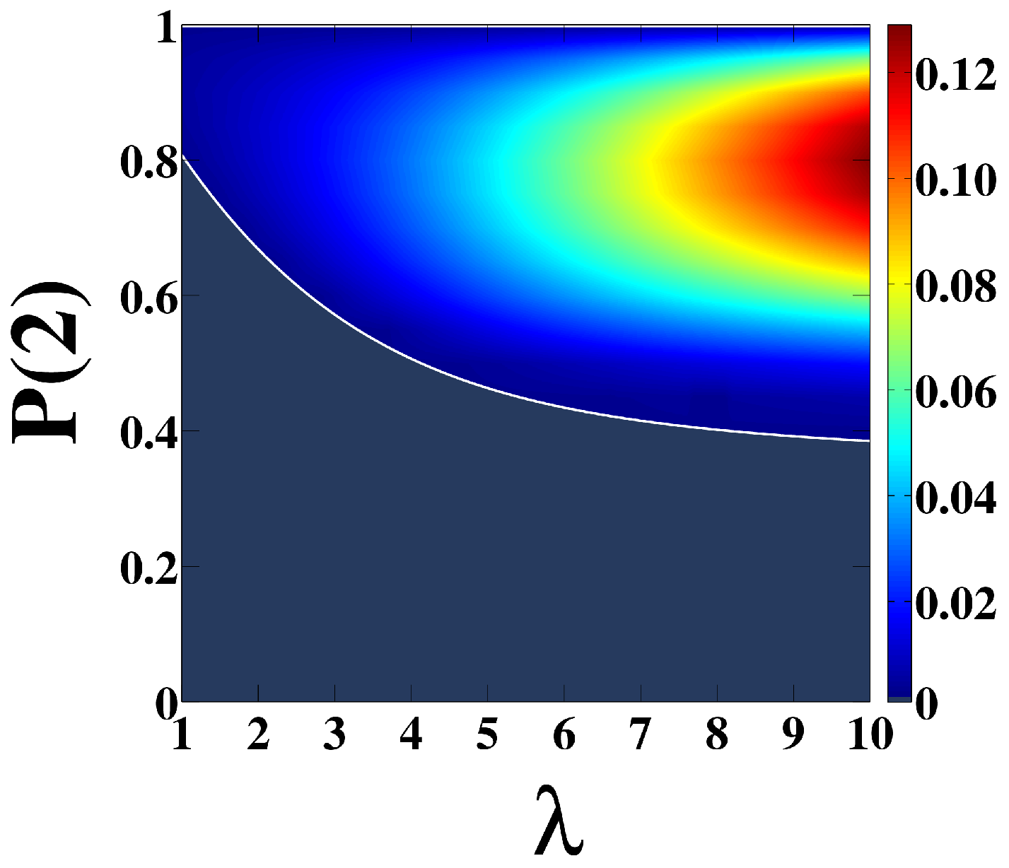
In Fig. 7 we show the phase diagram pointing out the fraction of driver nodes as a function of the parameters and . The dark grey area defines the region where the zero-energy solution is stable, hence the network has an infinitesimal fraction of driver nodes (). Outside this region, the minimum fraction of driver nodes necessary for a full network control is displayed (lowest stable solution of the MS equations).
Appendix F Improving the controllability of Poisson networks
In the main text of the paper we have described an algorithm that can improve the controllability of networks by adding links to it and reducing the number of nodes with in-degree and out-degree smaller than 3. While in the main text we show that such algorithm can be used to improve the controllability of scale-free networks, here we show that the same algorithm can be used to improve the controllability also of Poisson networks. In fact this approach can be applied to networks with any type of degree distribution.
In Figure 8 we display the fraction of driver nodes when we add links in the network divided by its initial value where the network has a Poisson degree distribution and average degree . We note that in this case the fraction of links that need to be added to have full controllability is of the order of . Here we have chosen to display the efficiency instead of the average distance because the network, specially at the beginning, is not fully connected.
When the displayed network has and it becomes fully controllable.

References
- [1] J.-J. Slotine ,W. Li W. Applied Nonlinear Control (Prentice-Hall, 1991).
- [2] X. F. Wang, G. Chen, Physica A 310, 521 (2002).
- [3] F. Sorrentino, M. di Bernardo, F. Garofalo, G. Chen, Phys. Rev. E 75, 1 (2007).
- [4] R. Gutiérrez,I. Sendiña-Nadal, M. Zanin, D. Papo, S. Boccaletti, Sci. Rep. 2 (2007).
- [5] C.-T. Lin, IEEE Trans. Auto. Contr. 19, 201 (1974).
- [6] Y.-Y. Liu, J.-J. Slotine, A.-L. Barabási, Nature 473, 167 (2011).
- [7] P. Márton, Y.-Y. Liu, J.-J. Slotine, A.-L. Barabási, Scientific Reports 3 (2013).
- [8] W.-X. Wang, X. Ni, Y.-C. Lai, C. Grebogi, Phys. Rev. E 85, 026115 (2012).
- [9] G. Yan, J. Ren, Y.-C. Lai, C.H. Lai, B. Li Phys. Rev. Lett. 108, 218703 (2012).
- [10] T. Nepusz, T. Vicsek, Nature Phys. 8, 568 (2012).
- [11] P. Csermely, et al. Pharmacology & therapeutics 138, 333 (2013)
- [12] E. Bullmore, O. Sporns, Nature Reviews Neuroscience 10, 186 (2009).
- [13] P. Bonifazi, et al. , Science 326, 1419 (2009).
- [14] J. D. Power et al. , Neuron 72, 665 (2011).
- [15] D. Delpini et al. , Scientific Reports 3, 1626 (2012).
- [16] R. Albert and A.-L. Barabási, Rev. Mod. Phys. 74, 47 (2002).
- [17] M. E. J. Newman, SIAM Review 45, 167 (2003).
- [18] S. Boccaletti, V. Latora, Y. Moreno, M. Chavez, and D.-U. Hwang, Phys. Reports 424, 175 (2006).
- [19] Caldarelli G. Scale-Free Networks: Complex Webs in Nature and Technology (Oxford University Press, Oxford, 2007).
- [20] S. N. Dorogovtsev, A. V. Goltsev, and J. F. F. Mendes, Rev. Mod. Phys. 80, 1275 (2008).
- [21] A. Barrat, M. Barthélemy, and A. Vespignani, Dynamical Processes on Complex Networks (Cambridge University Press, Cambridge, 2008).
- [22] L. Zdeborová and M. Mézard, J. Stat Mech. P05003 (2006).
- [23] F. Altarelli, A. Braunstein, A. Ramezanpour, and R. Zecchina, Phys. Rev. Lett. 106, 190601 (2011).
- [24] M. Mézard, G. Parisi, Eur. Phys. J. B 20,217 (2001).
- [25] O. C.Martin, R. Monasson, and R. Zecchina,Theoretical computer science 265, 3 (2001).
- [26] A. K. Hartmann and M. Weigt, Phase Transitions in Combinatorial Optimization Problems, (WILEY-VCH, Weinheim, 2005).
- [27] M. Mézard, A. Montanari Information, physics and computation (Oxford University Press, Oxford, 2009).
- [28] T. Jia, Y.-Y. Liu, E. Csóka, M. Pósfai, J.-J. Slotine, A.-L. Barabási Nature Communications 4, 1 (2013).
- [29] M. Boguñá, R. Pastor-Satorras, A. Vespignani, Eur. Phys. J. B 38, 205 (2004).
- [30] H. Seyed-Allaei, G. Bianconi, M. Marsili, Phys. Rev. E 73, 046113 (2006).
- [31] See the Appendix.
- [32] J.E. Hopcroft, and R. M. Karp, SIAM Journal on Computing 2(4): 225231(1973).
- [33] A. Montanari and F. Ricci-Tersenghi, Eur. Phys. J. B 33, 339 (2003).
- [34] O. Rivoire, G. Biroli, O. C. Martin, and M. Mézard (2004). Eur. Phys. J. B 37: 55-78.
- [35] C. Lucibello and F. Ricci-Tersenghi, Int. J. Stat. Mech., Vol. 2014, 136829 (2014).
- [36] T. Castellani, F. Krzakala, and F. Ricci-Tersenghi, Eur. Phys. J. B 47, 99-108 (2005).