Toeplitz operators and the Roe-Higson type index theorem in Riemannian surfaces

Tatsuki SETO Address: Graduate School of Mathematics, Nagoya University, Furocho, Chikusaku, Nagoya, Japan Email address: m11034y@math.nagoya-u.ac.jp

Abstract.

We study a two dimensional analogue of the Roe-Higson index theorem for a partitioned manifold. We prove that Connes’ pairing of some invertible element with Roe’s cyclic one-cocycle coincides to the Fredholm index of a Toeplitz operator. In the proof of this paper, we use some properties of a circle and use Higson’s argument. In the last section, there is a example of partitioned manifold, which is not a cylinder, with non-trivial pairing.

Introduction

Let $M$ be a partitioned complete Riemannian manifold, that is, there exist codimension zero submanifolds with boundary $M^{\pm}$ and a codimension one closed submanifold $N$ such that $M=M^{+}\cup M^{-}$ and $N=M^{+}\cap M^{-}=\partial M^{+}=\partial M^{-}$ . Let $S\to M$ be a Clifford bundle in the sense of [12, Definition 3.4] and let $D$ be the Dirac operator of $S$ . Let $S_{N}$ be the restriction on $N$ of $S$ . Then we can assume $S_{N}$ is a graded Clifford bundle over $N$ . Let $D_{N}$ be the graded Dirac operator of $S_{N}$ . In the above setting, we denote by $u_{D}$ the Cayley transform of $D$ , that is, $u_{D}:=(D-i)(D+i)^{-1}$ . Then $u_{D}$ is a invertible element in the Roe algebra $C^{\ast}(M)$ . In [11], Roe defined the odd index class odd-ind $(D)\in K_{1}(C^{\ast}(M))$ , which is represented by $u_{D}$ , and he also defined the cyclic one-cocycle $\zeta$ , which is called the Roe cocycle, on a dense subalgebra of $C^{\ast}(M)$ . Then Connes’ pairing of cyclic cohomology with $K$ -theory $\langle u_{D},\zeta\rangle$ is agree up to constant with the Fredholm index of $D_{N}^{+}$ [11]. In [8], Higson gave a very simple and clear proof of this theorem. So we call that this theorem is the Roe-Higson index theorem.

When $M$ is even dimensional, $\mathrm{index}(D_{N}^{+})$ is always zero in the Roe-Higson index theorem. So we want to get another non trivial formula. On the other hand, Toeplitz operators play a role of fundamental operators in the Atiyah-Singer index theorem on odd dimensional closed manifolds [1, §20, 24]. Therefore we shall prove another index theorem with Toeplitz operators on $N$ . Namely, we shall prove Connes’ pairing of the Roe cocyle with another $K_{1}$ -element $[u_{\phi}]$ (see Proposition 1.4) is agree with the Fredholm index of a Toeplitz operator on $N$ (Theorem 1.9).

Main Theorem .

Let $M$ be a partitioned oriented Riemannian surface. Let $S$ be a graded spin bundle over $M$ with $\mathbb{Z}_{2}$ -grading $\epsilon$ and let $D$ be the graded Dirac operator on $M$ . We assume $\phi\in C^{1}(M\,;\,GL_{l}(\mathbb{C}))$ satisfies $\|\phi\|<\infty$ , $\|grad(\phi)\|<\infty$ and $\|\phi^{-1}\|<\infty$ . Define

u_{\phi}:=(D+\epsilon)^{-1}\begin{bmatrix}\phi&0\\ 0&1\end{bmatrix}(D+\epsilon).

Then the following formula holds:

\left\langle[u_{\phi}],\zeta\right\rangle=-\frac{1}{8\pi i}\mathrm{index}(T_{\phi}).

The main strategy of the proof of our main theorem is to reduce the general two dimensional case to the $\mathbb{R}\times S^{1}$ case by similar argument of Higson in [8]. To prove the $\mathbb{R}\times S^{1}$ case, we can use the family of very useful functions $\{e^{ikx}\}_{k}$ , which is orthonormal basis of $L^{2}(S^{1})$ , all eigenvectors of Dirac operator $-i\partial/\partial x$ on $S^{1}$ , and all representative elements of fundamental group $\pi_{1}(S^{1})$ .

The general dimensional case of our main theorem is in [13]. It contains the $KK$ -theoretic construction of $[u_{\phi}]$ .

1. Main Theorem

1.1. Elements of the $K_{1}$ group

In this subsection, we define $K_{1}$ elements used in our main theorem.

Definition 1.1.

Let $M$ be a oriented complete Riemannian manifold. We assume that the triple $(M^{+},M^{-},N)$ satisfies the following conditions:

•

$M^{+}$ and $M^{-}$ are two codimension zero submanifolds of $M$ with boundary,
•

$M=M^{+}\cup M^{-}$ ,
•

$N$ is a codimension one closed submanifold of $M$ ,
•

$N=M^{+}\cap M^{-}=-\partial M^{+}=\partial M^{-}$ .

Then we call that $(M^{+},M^{-},N)$ is a partition of $M$ . Then we call that $M$ is a partitioned manifold.

Refer to caption — Figure 1. Partitioned manifold

In this paper, we assume that $M$ is a partitioned oriented two dimensional complete Riemannian manifold (i.e. complete Riemannian surface) and $(M^{+},M^{-},N)$ is a partition of $M$ . Let $S$ be a graded spin bundle of $M$ ¹¹ 1 Every orientable surfaces are spin [10, p.88]. with grading $\epsilon$ and a Clifford action $c$ . Let $D$ be the graded Dirac operator of $S$ . For simplicity, we assume that $M$ is connected and $N$ is isometric to the unit circle $S^{1}$ . We also assume $c(\mathrm{d}/\mathrm{d}t)c(\mathrm{d}/\mathrm{d}x)=\begin{bmatrix}i&0\\ 0&-i\end{bmatrix}$ on $(-\epsilon,\epsilon)\times N$ of tubular neighborhood of $N$ , where $\{\mathrm{d}/\mathrm{d}t,\mathrm{d}/\mathrm{d}x\}$ is a positively oriented orthonormal vector fields on $(-\epsilon,\epsilon)\times N$ .

Remark 1.2.

In particular, we assume $M$ is non compact, then $S$ is trivial bundle: $S=M\times\mathbb{C}^{2}$ . Especially, if $M=\mathbb{R}^{2}\cong\mathbb{C}$ with standard metric, then

D=2\begin{bmatrix}0&-\partial/\partial\bar{z}\\ \partial/\partial z&0\end{bmatrix}.

Let $\mathcal{L}(L^{2}(S))$ be the set of all bounded operators on $L^{2}$ -sections of $S$ . Let $C^{\ast}(M)$ be the Roe algebra of $M$ , that is, $C^{\ast}(M)$ is the completion in $\mathcal{L}(L^{2}(S))$ of the $\ast$ -algebra of all bounded integral operators on $L^{2}(S)$ with a smooth kernel and finite propagation [11, p.191]. We collect some well-known properties of the Roe algebra which we use.

Proposition 1.3.

[9, 11] We assume that $M$ , $S$ , and $D$ are as above. The following holds.

$(1)$

Let $f\in C_{0}(\mathbb{R})$ be a continuous function on $\mathbb{R}$ with vanishing at infinity and let $\lambda\in\mathbb{R}$ . Define $D^{\prime}:=D+\begin{bmatrix}0&\lambda\\ \lambda&0\end{bmatrix}$ , then $f(D^{\prime})\in C^{\ast}(M)$ .
$(2)$

Let $D^{\ast}(M)$ be the unital $C^{\ast}$ -algebra generated by all pseudolocal operators on $L^{2}(S)$ ²² 2 $T\in\mathcal{L}(L^{2}(S))$ is pseudolocal if $[f,T]\sim 0$ for all $f\in C_{0}(M)$ , that is, $[f,T]$ is compact. with finite propagation. Then $C^{\ast}(M)$ is a closed $\ast$ -bisided ideal of $D^{\ast}(M)$ .
$(3)$

$fu\sim 0$ and $uf\sim 0$ for all $u\in C^{\ast}(M)$ and $f\in C_{0}(M)$ .
$(4)$

Let $\varpi$ be the characteristic function of $M^{+}$ . Then $[\varpi,u]\sim 0$ for all $u\in C^{\ast}(M)$ .

By using above properties, we define a $K_{1}$ -element.

Proposition 1.4.

Let $\phi\in C^{1}(M;GL_{l}(\mathbb{C}))$ be a continuously differentiable map from $M$ to general linear group $GL_{l}(\mathbb{C})$ . We assume that $\|\phi\|<\infty$ , $\|grad(\phi)\|<\infty$ and $\|\phi^{-1}\|<\infty$ . Define

u_{\phi}:=(D+\epsilon)^{-1}\begin{bmatrix}\phi&0\\ 0&1\end{bmatrix}(D+\epsilon),

then $u_{\phi}-\begin{bmatrix}1&0\\ 0&\phi\end{bmatrix}\in M_{l}(C^{\ast}(M))$ .

Proof.

It suffices to show the $l=1$ case. Firstly, $(D+\epsilon)^{-1}\in C^{\ast}(M)$ and $\|(D+\epsilon)^{-1}\|\leq 2$ since $(D+\epsilon)^{-1}=(D^{2}+1)^{-1}(D+\epsilon)\in C^{\ast}(M)$ . On the other hand,

	$\displaystyle u_{\phi}\sigma$	$\displaystyle=(D+\epsilon)^{-1}\begin{bmatrix}\phi&0\\ 0&1\end{bmatrix}\begin{bmatrix}1&D^{-}\\ D^{+}&-1\end{bmatrix}\sigma$
		$\displaystyle=(D+\epsilon)^{-1}\begin{bmatrix}\phi&D^{-}\phi-D^{-}\phi+\phi D^{-}\\ D^{+}&-1\end{bmatrix}\sigma$
		$\displaystyle=(D+\epsilon)^{-1}\left((D+\epsilon)\begin{bmatrix}1&0\\ 0&\phi\end{bmatrix}+\begin{bmatrix}\phi-1&[\phi,D^{-}]\\ 0&\phi-1\end{bmatrix}\right)\sigma$
		$\displaystyle=\begin{bmatrix}1&0\\ 0&\phi\end{bmatrix}\sigma+(D+\epsilon)^{-1}\begin{bmatrix}\phi-1&-c(grad(\phi))^{-}\\ 0&\phi-1\end{bmatrix}\sigma,$

for any $\sigma\in C^{\infty}_{c}(S)$ , where $c(grad(\phi))^{-}$ is the negative part of the Clifford action of $grad(\phi)$ . So

\|u_{\phi}\sigma\|_{L^{2}}\leq 3(\|\phi\|+\|grad(\phi)\|+1)\|\sigma\|_{L^{2}}.

Thus $u_{\phi}$ can be extended uniquely as a bounded operator on $L^{2}(S)$ since $C^{\infty}_{c}(S)$ is dense in $L^{2}(S)$ , and $u_{\phi}-\begin{bmatrix}1&0\\ 0&\phi\end{bmatrix}\in C^{\ast}(M)$ . ∎

Let $C_{b}(M)$ be the set of all bounded continuous functions on $M$ . We assume that $C^{\ast}_{b}(M):=C^{\ast}(M)+C_{b}(M)$ is a unital $C^{\ast}$ -subalgebra of $\mathcal{L}(L^{2}(S))$ . By this proposition, $u_{\phi}$ is invertible in $M_{l}(C^{\ast}_{b}(M))$ with $(u_{\phi})^{-1}=u_{\phi^{-1}}$ . So we can consider $[u_{\phi}]\in K_{1}(C^{\ast}_{b}(M))$ .

1.2. Cyclic cocycle and pairing

Let $\varpi$ be the characteristic function of $M^{+}$ , and $\chi:=2\varpi-1$ . We note that $[\chi,u]$ is a compact operator for all $u\in C^{\ast}_{b}(M)$ since $[\chi,f]=0$ for all $f\in C_{b}(M)$ . We define the Banach algebra

\mathscr{A}_{b}:=\{A\in C^{\ast}_{b}(M)\,;\,[\chi,A]\text{ is a trace class operator}\}

with norm $\|A\|_{\mathscr{A}_{b}}:=\|A\|+\|[\chi,A]\|_{1}$ , where $\|\cdot\|$ is a operator norm on $L^{2}(S)$ and $\|\cdot\|_{1}$ is a trace norm. We define a cyclic cocycle on $\mathscr{A}_{b}$ and take the pairing of it with $K_{1}(C^{\ast}_{b}(M))$ .

Proposition 1.5.

[11, Proposition 1.6] For any $A,B\in\mathscr{A}_{b}$ , we define

\zeta(A,B):=\frac{1}{4}\mathrm{Tr}(\chi[\chi,A][\chi,B]).

Then $\zeta$ is a cyclic one-cocycle on $\mathscr{A}_{b}$ . We call that $\zeta$ is the Roe cocycle.

To take Connes’ pairing of the Roe cocycle $\zeta$ with $K_{1}(C^{\ast}_{b}(M))$ , we use a next fact.

Proposition 1.6.

[4, p.92] $\mathscr{A}_{b}$ is dense and closed under holomorphic functional calculus in $C^{\ast}_{b}(M)$ . So the inclusion $i:\mathscr{A}_{b}\to C^{\ast}_{b}(M)$ induces the isomorphism $i_{\ast}:K_{1}(\mathscr{A}_{b})\cong K_{1}(C^{\ast}_{b}(M))$ .

Proof.

Let $\mathscr{X}$ be the $\ast$ -algebra of all integral operators on $L^{2}(S)$ with a smooth kernel and finite propagation speed. Then, $\mathscr{X}_{b}:=\mathscr{X}+C_{b}(M)$ is a dense subalgebra in $C^{\ast}_{b}(M)$ and $\mathscr{X}_{b}\subset\mathscr{A}_{b}$ [11, Proposition 1.6]. So $\mathscr{A}_{b}$ is dense in $C^{\ast}_{b}(M)$ .

The rest of proof is in [4, p.92]. ∎

Using this proposition, we can take the pairing of the Roe cocycle with $K_{1}(C^{\ast}_{b}(M))$ through the isomorphism $i_{\ast}:K_{1}(\mathscr{A}_{b})\cong K_{1}(C^{\ast}_{b}(M))$ as follows:

Definition 1.7.

[4, p.109] Define the map

\langle\cdot,\zeta\rangle:K_{1}(C^{\ast}_{b}(M))\to\mathbb{C}

by $\langle[u],\zeta\rangle:=\frac{1}{8\pi i}\sum_{i,j}\zeta((u^{-1})_{ji},u_{ij})$ , where we assume $[u]$ is represented by a element of $GL_{n}(\mathscr{A}_{b})$ and $u_{ij}$ is the $(i,j)$ -component of $u$ . We note that this is Connes’ pairing of cyclic cohomology with $K$ -theory, and $\frac{1}{8\pi i}$ is a constant of the pairing.

The goal of this paper is to prove that the result of this pairing with $[u_{\phi}]$ is the Fredholm index of a Toeplitz operator.

1.3. Toeplitz operators

We review Toeplitz operators on $S^{1}$ to fix notations.

Proposition 1.8.

[6] Let $\phi\in C(S^{1}\,;\,GL_{l}(\mathbb{C}))$ be a continuous map from $S^{1}$ to $GL_{l}(\mathbb{C})$ . Define $\mathcal{H}:=\mathrm{Span}_{\mathbb{C}}\{e^{ikx}\,;\,k=0,1,2,\dots\}\subset L^{2}(S^{1})$ ³³ 3 $\mathcal{H}$ is called the Hardy space. and let $P:L^{2}(S^{1})\to\mathcal{H}$ be the projection. Then for any $f\in\mathcal{H}^{l}$ , we define Toeplitz operator $T_{\phi}:\mathcal{H}^{l}\to\mathcal{H}^{l}$ by $T_{\phi}f:=P\phi f$ . Then $T_{\phi}$ is a Fredholm operator and $\mathrm{index}(T_{\phi})=-\mathrm{deg}(\det(\phi))$ , where $\mathrm{deg}(\det(\phi))$ is the degree of the map $\det(\phi):S^{1}\to\mathbb{C}^{\times}$ .

We note that the Hardy space $\mathcal{H}$ is a positive eigenspace of $-i\partial/\partial x$ , which is a Dirac operator on $S^{1}$ . See also [2, p.160].

1.4. Main theorem

Using above notation, we state our main theorem as follows.

Theorem 1.9.

We also denote by $\phi$ the restriction on $N$ of $\phi$ . Then the following formula holds:

\left\langle[u_{\phi}],\zeta\right\rangle=-\frac{1}{8\pi i}\mathrm{index}(T_{\phi}).

By the index theorem of Toeplitz operators (Proposition 1.8), right hand side of this formula is calculated by some geometric invariant of the mapping degree. So this theorem is a kind of index theorem (see also next section):

Corollary 1.10.

Using above notation,

\mathrm{index}(\varpi u_{\phi}\varpi:\varpi(L^{2}(S))^{l}\to\varpi(L^{2}(S))^{l})=-\mathrm{deg}(\det(\phi)).

2. The pairing and the Fredholm index

To prove Theorem 1.9, we firstly describe $\zeta(u^{-1},u)=\sum_{i,j}\zeta((u^{-1})_{ji},u_{ij})$ by the Fredholm index of some Fredholm operator.

Proposition 2.1.

[5, IV.1] For any $u\in GL_{n}(\mathscr{A}_{b})$ ,

\zeta(u^{-1},u)=-\mathrm{index}(\varpi u\varpi:\varpi(L^{2}(S))^{n}\to\varpi(L^{2}(S))^{n}).

Proof.

Since $u\in GL_{n}(\mathscr{A}_{b})$ and

\varpi-\varpi u^{-1}\varpi u\varpi=-\varpi[\varpi,u^{-1}][\varpi,u]\varpi,

so $\varpi-\varpi u^{-1}\varpi u\varpi$ and $\varpi-\varpi u\varpi u^{-1}\varpi$ are trace class operators on $\varpi(L^{2}(S))^{n}$ . Therefore we get

\mathrm{index}(\varpi u\varpi:\varpi(L^{2}(S))^{n}\to\varpi(L^{2}(S))^{n})=\mathrm{Tr}(\varpi-\varpi u^{-1}\varpi u\varpi)-\mathrm{Tr}(\varpi-\varpi u\varpi u^{-1}\varpi)

by [4, p.88]. So we get

		$\displaystyle\mathrm{index}(\varpi u\varpi:\varpi(L^{2}(S))^{n}\to\varpi(L^{2}(S))^{n})=\frac{1}{4}\mathrm{Tr}(\chi[\chi,u][\chi,u^{-1}])$
	$\displaystyle=$	$\displaystyle\frac{1}{4}\sum_{i,j}\mathrm{Tr}(\chi[\chi,u_{ij}][\chi,(u^{-1})_{ji}])=-\zeta(u^{-1},u).$

∎

By this proposition and homotopy invariance of Fredholm indices, we get the following formula of our pairing and the Fredholm index:

(1)

\left\langle[u_{\phi}],\zeta\right\rangle=-\frac{1}{8\pi i}\mathrm{index}(\varpi u_{\phi}\varpi:\varpi(L^{2}(S))^{l}\to\varpi(L^{2}(S))^{l}).

So we shall calculate this Fredholm index.

3. The $\mathbb{R}\times S^{1}$ case

In this section we shall prove the $M=\mathbb{R}\times S^{1}$ case, and in the next section we shall reduce the general case to $M=\mathbb{R}\times S^{1}$ case.

In this section we assume $M=\mathbb{R}\times S^{1}$ . $\mathbb{R}\times S^{1}$ is partitioned by $(\mathbb{R}_{+}\times S^{1},\mathbb{R}_{-}\times S^{1},S^{1})$ , where $\mathbb{R}_{\pm}:=\{t\in\mathbb{R}\,;\,t\geq 0~(\text{resp. }t\leq 0)\}$ . Then the Dirac operator $D$ of $S=\mathbb{R}\times S^{1}\times\mathbb{C}^{2}$ is given by the following formula:

D=\begin{bmatrix}0&-\partial/\partial t-i\partial/\partial x\\ \partial/\partial t-i\partial/\partial x&0\end{bmatrix},

where $(t,x)\in\mathbb{R}\times S^{1}$ . Moreover, for any $\phi\in C^{1}(S^{1};GL_{l}(\mathbb{C}))$ , define $\phi(t,x):=\phi(x)$ on $\mathbb{R}\times S^{1}$ .

3.1. Homotopy

To calculate $\mathrm{index}(\varpi u_{\phi}\varpi:\varpi(L^{2}(S))^{l}\to\varpi(L^{2}(S))^{l})$ , we perturb this operator by a homotopy.

Proposition 3.1.

For any $s\in[0,1]$ , define

	$\displaystyle D_{s}$	$\displaystyle:=\begin{bmatrix}0&-\partial/\partial t+s/2-i\partial/\partial x\\ \partial/\partial t+s/2-i\partial/\partial x&0\end{bmatrix}=D+\begin{bmatrix}0&s/2\\ s/2&0\end{bmatrix}$
	$\displaystyle\text{and~}u_{\phi,s}$	$\displaystyle:=(D_{s}+(1-s)\epsilon)^{-1}\begin{bmatrix}\phi&0\\ 0&1\end{bmatrix}(D_{s}+(1-s)\epsilon).$

Then $[0,1]\ni s\mapsto u_{\phi,s}\in\mathcal{L}(L^{2}(S)^{l})$ is continuous and $u_{\phi,s}-\begin{bmatrix}1&0\\ 0&\phi\end{bmatrix}\in M_{l}(C^{\ast}(M))$ .

Proof.

It suffices to show the $l=1$ case. We note that $\|D_{s}f\|_{L^{2}}\geq s\|f\|_{L^{2}}/2$ for any $f\in domain(D_{s})=domain(D)$ and $s\in(0,1]$ . Moreover $D_{s}$ is self-adjoint. Therefore the spectrum of $D_{s}$ and $(-s/2,s/2)$ are disjoint, especially $D_{1}^{-1}\in\mathcal{L}(L^{2}(S))$ .

Since $(D_{s}+(1-s)\epsilon)^{2}=D_{s}^{2}+(1-s)^{2}$ , so $(D_{s}+(1-s)\epsilon)^{-1}\in C^{\ast}(M)$ . Therefore $u_{\phi,s}$ is well-defined as a densely defined closed operator of $domain(u_{\phi,s})=domain(D)$ . By similar proof of Proposition 1.4,

u_{\phi,s}=\begin{bmatrix}1&0\\ 0&\phi\end{bmatrix}+(D_{s}+(1-s)\epsilon)^{-1}\begin{bmatrix}(1-s)(\phi-1)&i\partial\phi/\partial x\\ 0&(1-s)(\phi-1)\end{bmatrix}

and $u_{\phi,s}-\begin{bmatrix}1&0\\ 0&\phi\end{bmatrix}\in C^{\ast}(M)$ .

Next we show $\|u_{\phi,s}-u_{\phi,s^{\prime}}\|\to 0$ as $s\to s^{\prime}$ for all $s^{\prime}\in[0,1]$ . First, we show that $\{\|(D_{s}+(1-s)\epsilon)^{-1}\|\}_{s\in[0,1]}$ is a bounded set. Set $f_{s}(x):=\left|\frac{x}{x^{2}+(1-s)^{2}}\right|$ and $g_{s}(x):=\left|\frac{1}{x^{2}+(1-s)^{2}}\right|$ . By fundamental calculus, we can show that

\sup_{|x|\geq s/2}\left|f_{s}(x)\right|\leq\frac{5}{2}\text{~~~\ and~}\sup_{|x|\geq s/2}\left|g_{s}(x)\right|\leq\frac{5}{4}.

Therefore

	$\displaystyle\\|(D_{s}+(1-s)\epsilon)^{-1}\\|$	$\displaystyle\leq\\|(D_{s}^{2}+(1-s)^{2})^{-1}D_{s}\\|+\\|(1-s)(D_{s}^{2}+(1-s)^{2})^{-1}\\|$
		$\displaystyle\leq\sup_{\|x\|\geq s/2}\left\|f_{s}(x)\right\|+\sup_{\|x\|\geq s/2}\left\|g_{s}(x)\right\|\leq 15/4$

for all $s\in[0,1]$ .

On the other hand,

	$\displaystyle u_{\phi,s}-u_{\phi,s^{\prime}}=$	$\displaystyle\{(D_{s}+(1-s)\epsilon)^{-1}-(D_{s^{\prime}}+(1-s^{\prime})\epsilon)^{-1}\}\begin{bmatrix}(1-s)(\phi-1)&i\phi^{\prime}\\ 0&(1-s)(\phi-1)\end{bmatrix}$
		$\displaystyle+(D_{s^{\prime}}+(1-s^{\prime})\epsilon)^{-1}\begin{bmatrix}(s^{\prime}-s)(\phi-1)&0\\ 0&(s^{\prime}-s)(\phi-1)\end{bmatrix}$

and the second term converges to $0$ in operator norm topology as $s\to s^{\prime}$ , so we should only show that $\|(D_{s}+(1-s)\epsilon)^{-1}-(D_{s^{\prime}}+(1-s^{\prime})\epsilon)^{-1}\|\to 0$ as $s\to s^{\prime}$ . But this is proved by above uniformly boundness as follows:

		$\displaystyle\\|(D_{s}+(1-s)\epsilon)^{-1}-(D_{s^{\prime}}+(1-s^{\prime})\epsilon)^{-1}\\|$
	$\displaystyle=$	$\displaystyle\\|(D_{s}+(1-s)\epsilon)^{-1}((s-s^{\prime})\epsilon+D_{s^{\prime}}-D_{s})(D_{s^{\prime}}+(1-s^{\prime})\epsilon)^{-1}\\|$
	$\displaystyle\leq$	$\displaystyle\frac{3}{2}\|s-s^{\prime}\|\\|(D_{s^{\prime}}+(1-s^{\prime})\epsilon)^{-1}\\|\\|(D_{s}+(1-s)\epsilon)^{-1}\\|$
	$\displaystyle\leq$	$\displaystyle 32\|s-s^{\prime}\|\to 0.$

∎

By this proposition, we get

\mathrm{index}(\varpi u_{\phi}\varpi)=\mathrm{index}(\varpi u_{\phi,0}\varpi)=\mathrm{index}(\varpi u_{\phi,1}\varpi).

Since

\varpi u_{\phi,1}\varpi=\begin{bmatrix}\varpi&0\\ 0&\varpi(-\partial/\partial t+1/2-i\partial/\partial x)^{-1}\phi(-\partial/\partial t+1/2-i\partial/\partial x)\varpi\end{bmatrix}\left(=:\begin{bmatrix}\varpi&0\\ 0&\mathscr{T}_{\phi}\end{bmatrix}\right),

so $\mathrm{index}(\varpi u_{\phi}\varpi)$ equals to

\mathrm{index}\Big(\mathscr{T}_{\phi}:\varpi(L^{2}(\mathbb{R}))\otimes L^{2}(S^{1})^{l}\to\varpi(L^{2}(\mathbb{R}))\otimes L^{2}(S^{1})^{l}\Big),

where we assume that $\varpi$ is the characteristic function of $\mathbb{R}_{+}$ .

3.2. The Hilbert transformation

Let $\mathscr{F}$ be the Fourier transformation:

\mathscr{F}[f](\xi):=\int_{\mathbb{R}}e^{-ix\xi}f(x)dx.

Let $H$ be the Hilbert transformation ⁴⁴ 4 The coefficient $i/\pi$ of the Hilbert transformation is usually $1/\pi$ . But we use this coefficient $i/\pi$ because of $H^{2}=1$ . :

Hf(t):=\frac{i}{\pi}\text{p.v.}\int_{\mathbb{R}}\frac{f(y)}{t-y}dy,

where p.v. is Cauchy’s principal value. Then we denote by $\hat{P}:L^{2}(\mathbb{R})\to\mathscr{H}_{-}$ the projection to the $-1$ -eigenspace $\mathscr{H}_{-}$ of $H$ , that is, $\hat{P}:=\frac{1}{2}(1-H)$ . Since $\mathscr{F}$ is a invertible operator from $\varpi(L^{2}(\mathbb{R}))$ to $\mathscr{H}_{-}$ , so

		$\displaystyle\mathrm{index}\Big(\mathscr{T}_{\phi}:\varpi(L^{2}(\mathbb{R}))\otimes L^{2}(S^{1})\to\varpi(L^{2}(\mathbb{R}))\otimes L^{2}(S^{1})\Big)$
	$\displaystyle=$	$\displaystyle\mathrm{index}\Big(\mathscr{F}\mathscr{T}_{\phi}\mathscr{F}^{-1}:\mathscr{H}_{-}\otimes L^{2}(S^{1})\to\mathscr{H}_{-}\otimes L^{2}(S^{1})\Big).$

Set

\hat{\mathscr{T}_{\phi}}:=\mathscr{F}\mathscr{T}_{\phi}\mathscr{F}^{-1}=\hat{P}(-it+1/2-i\partial/\partial x)^{-1}\phi(-it+1/2-i\partial/\partial x)\hat{P}^{\ast}.

To calculate the Fredholm index of $\hat{\mathscr{T}_{\phi}}$ , we use a basis of $L^{2}(\mathbb{R})$ made by eigenvectors of Hilbert transformation.

Proposition 3.2.

[14, Theorem 1] Set $\rho_{n}\in L^{2}(\mathbb{R})$ by

\rho_{n}(t):=\frac{(t-i)^{n}}{(t+i)^{n+1}}.

Then $\{\rho_{n}/\sqrt{\pi}\}$ is a orthonormal basis of $L^{2}(\mathbb{R})$ and

H\rho_{n}=\begin{cases}\rho_{n}&\text{if~}n<0\\ -\rho_{n}&\text{if~}n\geq 0\end{cases}.

By using this basis, we get $\mathscr{H}_{-}=\mathrm{Span}_{\mathbb{C}}\{\rho_{n}\,;\,n\geq 0\}$ and we can calculate following Fredholm indices, which is used in the next subsection.

Lemma 3.3.

For any $\alpha,\beta\neq 0$ , $\hat{P}\dfrac{t+i\beta}{t+i\alpha}\hat{P}^{\ast}\in\mathcal{L}(\mathscr{H}_{-})$ is a Fredholm operator and

\mathrm{index}\left(\hat{P}\frac{t+i\beta}{t+i\alpha}\hat{P}^{\ast}\right)=\begin{cases}0&\text{if~}\alpha\beta>0\\ -1&\text{if~}\alpha>0,\beta<0\\ 1&\text{if~}\alpha<0,\beta>0\end{cases}.

Proof.

Our proof of Fredholmness is similar to [3, p.99]. Let $c:\mathbb{R}\to S^{1}(\subset\mathbb{C})$ be the Cayley transformation defined by $c(t):=(t-i)(t+i)^{-1}$ . Define $\Phi(g)(t):=(t+i)^{-1}g(c(t))$ for any $g\in L^{2}(S^{1})$ . Then $\Phi:L^{2}(S^{1})\to L^{2}(\mathbb{R})$ is a invertible bounded linear operator with $\|\Phi\|=1/\sqrt{2}$ and $\Phi^{-1}(f)(z)=(c^{-1}(z)+i)f(c^{-1}(z))$ for all $f\in L^{2}(\mathbb{R})$ and $z\in S^{1}\setminus\{1\}$ .

Since $\Phi(e^{inx})=\rho_{n}$ , $\hat{P}f\hat{P}^{\ast}$ is a Fredholm operator on $\mathscr{H}_{-}$ for any $f\in C^{\infty}(\mathbb{R};\mathbb{C}^{\times})$ with $\lim_{t\to\infty}f(t)=\lim_{t\to-\infty}f(t)\in\mathbb{C}^{\times}$ . Now,

\left|\frac{t+i\beta}{t+i\alpha}\right|^{2}=\frac{t^{2}+\beta^{2}}{t^{2}+\alpha^{2}}>0

and $\lim_{t\to\pm\infty}\frac{t+i\beta}{t+i\alpha}=1$ . Therefore $\hat{P}\frac{t+i\beta}{t+i\alpha}\hat{P}^{\ast}$ is a Fredholm operator.

We calculate $\mathrm{index}(\hat{P}\frac{t+i\beta}{t+i\alpha}\hat{P}^{\ast})$ . Define $\mathrm{sgn}(\alpha):=\begin{cases}1&\text{if~}\alpha>0\\ -1&\text{if~}\alpha<0\end{cases}$ . Then we define a homotopy of Fredholm operators from $\hat{P}\frac{t+i\beta}{t+i\alpha}\hat{P}^{\ast}$ to $\hat{P}\frac{t+i\mathrm{sgn}(\beta)}{t+i\mathrm{sgn}(\alpha)}\hat{P}^{\ast}$ by

\hat{P}\frac{t+i(s\beta+(1-s)\mathrm{sgn}(\beta))}{t+i(s\alpha+(1-s)\mathrm{sgn}(\alpha))}\hat{P}^{\ast}

for $s\in[0,1]$ . Therefore

\mathrm{index}\left(\hat{P}\frac{t+i\beta}{t+i\alpha}\hat{P}^{\ast}\right)=\mathrm{index}\left(\hat{P}\frac{t+i\mathrm{sgn}(\beta)}{t+i\mathrm{sgn}(\alpha)}\hat{P}^{\ast}\right)=\begin{cases}0&\text{if~}\alpha\beta>0\\ -1&\text{if~}\alpha>0,\beta<0\\ 1&\text{if~}\alpha<0,\beta>0\end{cases}

by $\mathscr{H}_{-}=\mathrm{Span}_{\mathbb{C}}\{\rho_{n}\,;\,n\geq 0\}$ . ∎

3.3. The special case

Set $\phi_{k}(x)=e^{ikx}$ on $S^{1}$ for $k\in\mathbb{Z}$ . In this subsection, we calculate

\mathrm{index}(\hat{\mathscr{T}_{\phi_{k}}}:\mathscr{H}_{-}\otimes L^{2}(S^{1})\to\mathscr{H}_{-}\otimes L^{2}(S^{1}))

of the special case.

Proposition 3.4.

$\mathrm{index}(\varpi u_{\phi_{k}}\varpi)=\mathrm{index}(\hat{\mathscr{T}_{\phi_{k}}})=-k=\mathrm{index}(T_{\phi_{k}})$ .

Proof.

The first equality is proved in subsection 3.1 and 3.2, and the last equality is well known. So we should only show the second equality. Let $E_{\lambda}:=\mathbb{C}\{e^{i\lambda x}\}$ be the $\lambda$ -eigenspace of $-i\partial/\partial x$ . On $\mathscr{H}_{-}\otimes E_{\lambda}$ , operator $\hat{\mathscr{T}}_{\phi_{k}}$ acts as

\hat{P}(-it+1/2+\lambda+k)^{-1}(-it+1/2+\lambda)\hat{P}^{\ast}\otimes\phi_{k}

and $\hat{\mathscr{T}_{\phi_{k}}}(\mathscr{H}_{-}\otimes E_{\lambda})$ is contained in $\mathscr{H}_{-}\otimes E_{\lambda+k}$ . Therefore

		$\displaystyle\mathrm{index}(\hat{\mathscr{T}_{\phi_{k}}})$
	$\displaystyle=$	$\displaystyle\sum_{\lambda=-\infty}^{\infty}\mathrm{index}{\left(\hat{P}\frac{t+i(\lambda+1/2)}{t+i(\lambda+k+1/2)}\hat{P}^{\ast}\otimes\phi_{k}:\mathscr{H}_{-}\otimes E_{\lambda}\to\mathscr{H}_{-}\otimes E_{\lambda+k}\right)}$
	$\displaystyle=$	$\displaystyle-k$

by Lemma 3.3. ∎

3.4. The general case

Let $\phi\in C^{1}(S^{1};GL_{l}(\mathbb{C}))$ be a general continuously differentiable map. We reduce $\phi$ case to $\phi_{k}$ case.

Since the Gram-Schmidt orthogonalization $GL_{l}(\mathbb{C})\to U(l)$ is a homotopy equivalence map, so this map induces the isomorphism on fundamental groups $\pi_{1}(GL_{l}(\mathbb{C}))\cong\pi_{1}(U(l))$ . By the homotopy long exact sequence, this inclusion $i:C(S^{1};S^{1})\to C(S^{1};U(l))$ of $i(f):=\begin{bmatrix}f&0\\ 0&1_{l-1}\end{bmatrix}$ induces the isomorphism on fundamental groups $i_{\ast}:\pi_{1}(S^{1})\to\pi_{1}(U(l))$ [7, Example 4.55]. Moreover $\pi_{1}(S^{1})\cong\mathbb{Z}$ is represented by $\phi_{k}$ for all $k\in\mathbb{Z}$ . Therefore $\phi$ is homotopic to $\begin{bmatrix}\phi_{k}&0\\ 0&1_{l-1}\end{bmatrix}$ in $C(S^{1}\,;\,GL_{l}(\mathbb{C}))$ for some $k\in\mathbb{Z}$ . We denote $\psi_{s}$ by this homotopy. Moreover, since $C^{1}(S^{1})$ is dense and closed under holomorphic functional calculus in $C(S^{1})$ , so we can take this homotopy $\psi_{s}$ in $C^{1}(S^{1};GL_{l}(\mathbb{C}))$ .

Proposition 3.5.

$u_{\psi_{s}}$ is a continuous path in $\mathcal{L}(L^{2}(S)^{l})$ .

Proof.

By proof of Proposition 1.4,

u_{\psi_{s}}=\begin{bmatrix}1&0\\ 0&\psi_{s}\end{bmatrix}+(D+\epsilon)^{-1}\begin{bmatrix}\psi_{s}-1&i\psi_{s}^{\prime}\\ 0&\psi_{s}-1\end{bmatrix}.

Therefore

\|u_{\psi_{s}}-u_{\psi_{s^{\prime}}}\|\leq 3\|\psi_{s}-\psi_{s^{\prime}}\|_{C^{1}}\to 0

as $s\to s^{\prime}$ since $\psi_{s}$ is a path in $C^{1}(S^{1};GL_{l}(\mathbb{C}))$ . ∎

Proof of Theorem 1.9 of $M=\mathbb{R}\times S^{1}$ case.

By Proposition 3.5,

\mathrm{index}(\varpi u_{\phi}\varpi)=\mathrm{index}\left(\varpi\begin{bmatrix}u_{\phi_{k}}&0\\ 0&1_{l-1}\end{bmatrix}\varpi\right)=\mathrm{index}(\varpi u_{\phi_{k}}\varpi)

for some $k\in\mathbb{Z}$ . By Proposition 3.4, $\mathrm{index}(\varpi u_{\phi_{k}}\varpi)=\mathrm{index}(T_{\phi_{k}})$ . Moreover, since $\phi$ is homotopic to $\begin{bmatrix}\phi_{k}&0\\ 0&1_{l-1}\end{bmatrix}$ , so $\mathrm{index}(T_{\phi_{k}})=\mathrm{index}(T_{\phi})$ . Therefore $\mathrm{index}(\varpi u_{\phi}\varpi)=\mathrm{index}(T_{\phi})$ . We complete a proof of Theorem 1.9 by using (1) in section 2. ∎

4. The general two-manifold case

In this section we reduce the general two dimensional manifold case to the $\mathbb{R}\times S^{1}$ case. Our argument is similar to Higson’s argument in [8]. Firstly, we shall show cobordism invariance of the pairing.

Lemma 4.1.

[8, Lemma 1.4] Let $(M^{+},M^{-},N)$ and $(M^{+}{}^{\prime},M^{-}{}^{\prime},N^{\prime})$ be two partitions of $M$ . Then we assume these two partitions are cobordant, that is, the symmetric differences $M^{\pm}\triangle M^{\mp}{}^{\prime}$ are compact. Let $\varpi$ and $\varpi^{\prime}$ be the characteristic function of $M^{+}$ and $M^{+}{}^{\prime}$ , respectively. We assume $\phi\in C^{1}(M\,;\,GL_{l}(\mathbb{C}))$ satisfies $\|\phi\|<\infty$ , $\|grad(\phi)\|<\infty$ and $\|\phi^{-1}\|<\infty$ . Then $\mathrm{index}(\varpi u_{\phi}\varpi)=\mathrm{index}(\varpi^{\prime}u_{\phi}\varpi^{\prime})$ .

Proof.

It suffices to show the $l=1$ case. Since $[\phi,\varpi]=0$ and $[u_{\phi},\varpi]\sim 0$ , so

		$\displaystyle\mathrm{index}(\varpi u_{\phi}\varpi:\varpi(L^{2}(S))\to\varpi(L^{2}(S)))$
	$\displaystyle=$	$\displaystyle\mathrm{index}\left((1-\varpi)\begin{bmatrix}1&0\\ 0&\phi\end{bmatrix}+\varpi u_{\phi}\varpi:L^{2}(S)\to L^{2}(S)\right)$
	$\displaystyle=$	$\displaystyle\mathrm{index}\left((1-\varpi)\begin{bmatrix}1&0\\ 0&\phi\end{bmatrix}+\varpi u_{\phi}:L^{2}(S)\to L^{2}(S)\right)$
	$\displaystyle=$	$\displaystyle\mathrm{index}\left(\begin{bmatrix}1&0\\ 0&\phi\end{bmatrix}+\varpi v_{\phi}:L^{2}(S)\to L^{2}(S)\right),$

where we assume $v_{\phi}=u_{\phi}-\begin{bmatrix}1&0\\ 0&\phi\end{bmatrix}\in C^{\ast}(M)$ . Therefore we should only show $\varpi v_{\phi}\sim\varpi^{\prime}v_{\phi}$ . Now, since $M^{\pm}\triangle M^{\mp}{}^{\prime}$ are compact, there exists $f\in C_{0}(M)$ such that $\varpi-\varpi^{\prime}=(\varpi-\varpi^{\prime})f$ . So $\varpi v_{\phi}-\varpi^{\prime}v_{\phi}=(\varpi-\varpi^{\prime})fv_{\phi}\sim 0$ . ∎

Secondly, we shall reduce the general manifold case to the $\mathbb{R}\times N$ case used by Higson’s Lemma.

Lemma 4.2.

[8, Lemma 3.1] Let $M_{1}$ and $M_{2}$ be two partitioned oriented two dimensional complete Riemannian manifolds and let $S_{j}$ be a Hermitian vector bundle over $M_{j}$ . Let $\varpi_{j}$ be the characteristic function of $M_{j}^{+}$ . We assume that there exists an isometry $\gamma:M_{2}^{+}\to M_{1}^{+}$ which lifts an isomorphism $\gamma^{\ast}:S_{1}|_{M_{1}^{+}}\to S_{2}|_{M_{2}^{+}}$ . We denote again by $\gamma^{\ast}:\varpi_{1}(L^{2}(S_{1}))\to\varpi_{2}(L^{2}(S_{2}))$ the Hilbert space isometry defined by $\gamma$ . Then we assume $u_{j}\in GL_{l}(C^{\ast}(M_{j}))$ and $f_{j}\in GL_{l}(C_{b}(M_{j}))$ satisfy $v_{j}:=u_{j}-f_{j}\in M_{l}(C^{\ast}(M))$ and $\gamma^{\ast}u_{1}\varpi_{1}\sim\varpi_{2}u_{2}\gamma^{\ast}$ . Then $\mathrm{index}(\varpi_{1}u_{1}\varpi_{1})=\mathrm{index}(\varpi_{2}u_{2}\varpi_{2})$ .

Similarly, if there exists an isometry $\gamma:M_{2}^{-}\to M_{1}^{-}$ which lifts an isomorphism $\gamma^{\ast}:S_{1}|_{M_{1}^{-}}\to S_{2}|_{M_{2}^{-}}$ and $\gamma^{\ast}u_{1}\varpi_{1}\sim\varpi_{2}u_{2}\gamma^{\ast}$ , then $\mathrm{index}(\varpi_{1}u_{1}\varpi_{1})=\mathrm{index}(\varpi_{2}u_{2}\varpi_{2})$ .

Proof.

It suffices to show $l=1$ case. Let $v:(1-\varpi_{1})(L^{2}(S_{1}))\to(1-\varpi_{2})(L^{2}(S_{2}))$ be any invertible operator. Then $V:=\gamma^{\ast}\varpi_{1}+v(1-\varpi_{1}):L^{2}(S_{1})\to L^{2}(S_{2})$ is also invertible operator. Hence

		$\displaystyle\;V((1-\varpi_{1})+\varpi_{1}u_{1}\varpi_{1})-((1-\varpi_{2})+\varpi_{2}u_{2}\varpi_{2})V$
	$\displaystyle=$	$\displaystyle\;-\gamma^{\ast}\varpi_{1}+\varpi_{2}\gamma^{\ast}+\gamma^{\ast}\varpi_{1}u_{1}\varpi_{1}-\varpi_{2}u_{2}\varpi_{2}\gamma^{\ast}$
	$\displaystyle\sim$	$\displaystyle\;\gamma^{\ast}u_{1}\varpi_{1}-\varpi_{2}u_{2}\gamma^{\ast}\sim 0.$

Therefore $\mathrm{index}(\varpi_{1}u_{1}\varpi_{1})=\mathrm{index}(\varpi_{2}u_{2}\varpi_{2})$ since $V$ is an invertible operator and $\mathrm{index}(\varpi_{j}u_{j}\varpi_{j})=\mathrm{index}((1-\varpi_{j})+\varpi_{j}u_{j}\varpi_{j})$ for $j=1,2$ . ∎

In our case, we use this Lemma as follows:

Corollary 4.3.

Let $M_{j}$ be a Riemannian surface and let $S_{j}$ be a graded spin bundle over $M_{j}$ with grading $\epsilon_{j}$ . We assume that there exists an isometry $\gamma:M_{2}^{+}\to M_{1}^{+}$ which defines the Hilbert space isometry $\gamma^{\ast}:\varpi_{1}(L^{2}(S_{1}))\to\varpi_{2}(L^{2}(S_{2}))$ as in Lemma 4.2 and satisfies $D_{2}\gamma^{\ast}\sim\gamma^{\ast}D_{1}$ and $\epsilon_{2}\gamma^{\ast}\sim\gamma^{\ast}\epsilon_{1}$ on $\varpi_{1}(L^{2}(S_{1}))$ . Let $\phi_{j}\in C^{1}(M_{j}\,;\,GL_{l}(\mathbb{C}))$ satisfies $\|\phi_{j}\|<\infty$ , $\|grad(\phi_{j})\|<\infty$ and $\|\phi_{j}^{-1}\|<\infty$ as in Proposition 1.4 and $\phi_{1}$ and $\phi_{2}$ satisfy $\phi_{1}(\gamma(x))=\phi_{2}(x)$ for all $x\in M_{2}^{+}$ . Then $\mathrm{index}(\varpi_{1}u_{\phi_{1}}\varpi_{1})=\mathrm{index}(\varpi_{2}u_{\phi_{2}}\varpi_{2})$ .

Proof.

We should only show $\gamma^{\ast}u_{\phi_{1}}\varpi_{1}\sim\varpi_{2}u_{\phi_{2}}\gamma^{\ast}$ . Let $\varphi_{1}$ be a smooth function on $M_{1}$ such that $\mathrm{Supp}(\varphi_{1})\subset M_{1}^{+}$ and there exists a compact set $K_{1}\subset M_{1}$ such that $\varphi_{1}=\varpi_{1}$ on $M_{1}\setminus K_{1}$ . Define $\varphi_{2}(x):=\varphi_{1}(\gamma(x))$ for all $x\in M_{2}^{+}$ and $\varphi_{2}=0$ on $M_{2}^{-}$ . Then $\varphi_{2}$ is a smooth function on $M_{2}$ such that $\mathrm{Supp}(\varphi_{2})\subset M_{2}^{+}$ and there exists a compact set $K_{2}\subset M_{2}$ such that $\varphi_{2}=\varpi_{2}$ on $M_{2}\setminus K_{2}$ . Set $v_{\phi_{j}}=u_{\phi_{j}}-\begin{bmatrix}1&0\\ 0&\phi_{j}\end{bmatrix}$ . Then $\gamma^{\ast}v_{\phi_{1}}\varpi_{1}\sim\gamma^{\ast}v_{\phi_{1}}\varphi_{1}$ and $\varpi_{2}v_{\phi_{2}}\gamma^{\ast}\sim\varphi_{2}v_{\phi_{2}}\gamma^{\ast}$ . So if $\gamma^{\ast}v_{\phi_{1}}\varphi_{1}\sim\varphi_{2}v_{\phi_{2}}\gamma^{\ast}$ , then

\gamma^{\ast}u_{\phi_{1}}\varpi_{1}\sim\gamma^{\ast}v_{\phi_{1}}\varphi_{1}+\gamma^{\ast}\begin{bmatrix}1&0\\ 0&\phi_{1}\end{bmatrix}\varpi_{1}\sim\varphi_{2}v_{\phi_{2}}\gamma^{\ast}+\varpi_{2}\begin{bmatrix}1&0\\ 0&\phi_{2}\end{bmatrix}\gamma^{\ast}\sim\varpi_{2}u_{\phi_{2}}\gamma^{\ast}.

So we shall show $\gamma^{\ast}v_{\phi_{1}}\varphi_{1}\sim\varphi_{2}v_{\phi_{2}}\gamma^{\ast}$ . In fact,

		$\displaystyle\;\gamma^{\ast}v_{\phi_{1}}\varphi_{1}-\varphi_{2}v_{\phi_{2}}\gamma^{\ast}$
	$\displaystyle=$	$\displaystyle\;\gamma^{\ast}(D_{1}+\epsilon_{1})^{-1}\begin{bmatrix}\phi_{1}-1&-c(grad(\phi_{1}))^{-}\\ 0&\phi_{1}-1\end{bmatrix}\varphi_{1}-\varphi_{2}(D_{2}+\epsilon_{2})^{-1}\begin{bmatrix}\phi_{2}-1&-c(grad(\phi_{2}))^{-}\\ 0&\phi_{2}-1\end{bmatrix}\gamma^{\ast}$
	$\displaystyle=$	$\displaystyle\;\{\gamma^{\ast}(D_{1}+\epsilon_{1})^{-1}\varphi_{1}-\varphi_{2}(D_{2}+\epsilon_{2})^{-1}\gamma^{\ast}\}\begin{bmatrix}\phi_{1}-1&-c(grad(\phi_{1}))^{-}\\ 0&\phi_{1}-1\end{bmatrix}$
	$\displaystyle\sim$	$\displaystyle\;\{\gamma^{\ast}\varphi_{1}(D_{1}+\epsilon_{1})^{-1}-(D_{2}+\epsilon_{2})^{-1}\gamma^{\ast}\varphi_{1}\}\begin{bmatrix}\phi_{1}-1&-c(grad(\phi_{1}))^{-}\\ 0&\phi_{1}-1\end{bmatrix}$
	$\displaystyle=$	$\displaystyle\;(D_{2}+\epsilon_{2})^{-1}\{(D_{2}+\epsilon_{2})\gamma^{\ast}\varphi_{1}-\gamma^{\ast}\varphi_{1}(D_{1}+\epsilon_{1})\}(D_{1}+\epsilon_{1})^{-1}\begin{bmatrix}\phi_{1}-1&-c(grad(\phi_{1}))^{-}\\ 0&\phi_{1}-1\end{bmatrix}$
	$\displaystyle\sim$	$\displaystyle\;(D_{2}+\epsilon_{2})^{-1}\gamma^{\ast}[D_{1},\varphi_{1}](D_{1}+\epsilon_{1})^{-1}\begin{bmatrix}\phi_{1}-1&-c(grad(\phi_{1}))^{-}\\ 0&\phi_{1}-1\end{bmatrix}$
	$\displaystyle\sim$	$\displaystyle\;0$

since $grad(\varphi_{1})$ has a compact support and $[D_{1},\varphi_{1}]=c(grad(\varphi_{1}))$ . Thus we get $\gamma^{\ast}u_{\phi_{1}}\varpi_{1}\sim\varpi_{2}u_{\phi_{2}}\gamma^{\ast}$ . Therefore $\mathrm{index}(\varpi_{1}u_{\phi_{1}}\varpi_{1})=\mathrm{index}(\varpi_{2}u_{\phi_{2}}\varpi_{2})$ by Lemma 4.2. ∎

Proof of Theorem 1.9.

Firstly, let $a\in C^{\infty}([-1,1];[-1,1])$ satisfies

a(t)=\begin{cases}-1&\text{if~}-1\leq t\leq-3/4\\ 0&\text{if~}-2/4\leq t\leq 2/4\\ 1&\text{if~}3/4\leq t\leq 1\end{cases}.

Let $(-4\delta,4\delta)\times N$ be a tubular neighborhood of $N$ in $M$ satisfies

\sup_{(t,x),(s,y)\in[-3\delta,3\delta]\times N}|\phi(t,x)-\phi(s,y)|<\|\phi^{-1}\|^{-1}.

Define $\psi(t,x):=\phi(4\delta a(t),x)$ on $(-4\delta,4\delta)\times N$ and $\psi=\phi$ on $M\setminus(-4\delta,4\delta)\times N$ . Then $\psi\in C^{1}(M\,;\,GL_{l}(\mathbb{C}))$ and $\|\psi-\phi\|<\|\phi^{-1}\|^{-1}$ . Thus $[0,1]\ni t\mapsto\psi_{t}:=t\psi+(1-t)\phi$ satisfies $\psi_{t}\in C^{1}(M\,;\,GL_{l}(\mathbb{C}))$ , $\|\psi_{t}\|<\infty$ , $\|grad(\psi_{t})\|<\infty$ and $\|\psi_{t}^{-1}\|<\infty$ , $\|\psi_{t}-\psi_{t^{\prime}}\|\to 0$ and $\|grad(\psi_{t})-grad(\psi_{t^{\prime}})\|\to 0$ as $t\to t^{\prime}\in[0,1]$ . Therefore we should only show the case of which $\phi$ satisfies $\phi(t,x)=\phi(0,x)$ on tubular neighborhood $(-2\delta,2\delta)\times N$ . By Lemma 4.1 we may change a partition of $M$ to $(M^{+}\cup([-\delta,0]\times N),M^{-}\setminus((-\delta,0]\times N),\{-\delta\}\times N)$ without changing $\mathrm{index}(\varpi u_{\phi}\varpi)$ . Then by Corollary 4.3 we may change $M^{+}\cup([-\delta,0]\times N)$ to $[-\delta,\infty)\times N$ without changing $\mathrm{index}(\varpi u_{\phi}\varpi)$ where $\phi$ is changed to $\phi(t,x)=\phi(x)$ for $(t,x)\in(-\delta,0]\times N$ . We denote by $M^{\prime}:=([-\delta,\infty)\times N)\cup(M^{-}\setminus((-\delta,0]\times N))$ this manifold. Then $M^{\prime}$ is partitioned by $([-\delta,\infty)\times N,M^{-}\setminus((-\delta,0]\times N),\{-\delta\}\times N)$ . By using Lemma 4.1 and Corollary 4.3 again, we may change $M^{\prime}$ to $\mathbb{R}\times N$ without changing $\mathrm{index}(\varpi u_{\phi}\varpi)$ with similar argument as above where $\phi(t,x)=\phi(x)$ for $(t,x)\in\mathbb{R}\times N$ . Now we have changed $M$ to $\mathbb{R}\times N=\mathbb{R}\times S^{1}$ .

∎

5. Example

In this section, we see a example of a partitioned manifold with which the pairing $\langle[u_{\phi}],\zeta\rangle$ is not zero but it is not $\mathbb{R}\times S^{1}$ .

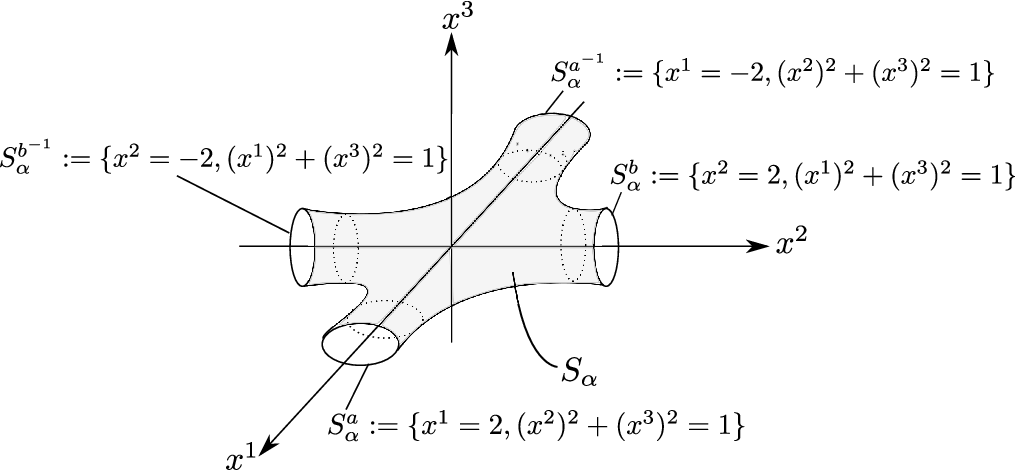
Firstly, we define partitioned two-manifold. Let $\Sigma_{2}$ be a closed Riemannian surface of genus two and let $C$ and $C^{\prime}$ be two submanifolds of $\Sigma_{2}$ which define generators of $H_{1}(\Sigma_{2};\mathbb{Z})$ as Figure 3. Moreover, we cut $\Sigma_{2}$ along $C$ and $C^{\prime}$ and embed to $\mathbb{R}^{3}$ like Figure 3.

Let $F_{2}:=\langle a,b\rangle$ be the free group with two generators. For all $\alpha\in F_{2}$ , we consider such surface $S_{\alpha}$ . Then we assume $S_{\alpha}$ is a oriented smooth manifold with Riemannian metric induced by $\mathbb{R}^{3}$ . Moreover we assume $T_{\alpha}^{g}(1/2)$ is a collar neighborhood of $S_{\alpha}^{g}$ in $S_{\alpha}$ for $g\in\{a,a^{-1},b,b^{-1}\}$ . Where for all $\delta>0$ , we define

T_{\alpha}^{a}(\delta):=\{2-\delta<x^{1}\leq 2,(x^{2})^{2}+(x^{3})^{2}=1\},

T_{\alpha}^{a^{-1}}(\delta):=\{-2\leq x^{1}<-2+\delta,(x^{2})^{2}+(x^{3})^{2}=1\},

T_{\alpha}^{b}(\delta):=\{2-\delta<x^{2}\leq 2,(x^{1})^{2}+(x^{3})^{2}=1\}\text{~, and}

T_{\alpha}^{b^{-1}}(\delta):=\{-2\leq x^{2}<-2+\delta,(x^{1})^{2}+(x^{3})^{2}=1\}.

Let $\phi_{\alpha}^{g}:\overline{T_{\alpha}^{g}(1/4)}\to[0,1/4]\times S^{1}$ be the orientation preserving isometry defined by identification of $\overline{T_{\alpha}^{g}(1/4)}$ with $[0,1/4]\times S^{1}$ . Define $M:=\bigsqcup_{\alpha}S_{\alpha}/\sim$ , where $x\sim y$ if (i) $x\in\overline{T_{\alpha}^{g}(1/4)}$ and $y\in\overline{T_{\beta}^{h}(1/4)}$ , (ii) $\alpha g=\beta h$ and (iii) $\phi_{\alpha}^{g}(x)=\phi_{\beta}^{h}(y)$ . Then $M$ is a oriented complete Riemannian manifold. Moreover, $F_{2}$ acts on $M$ freely. Let $\pi:M\to M/F_{2}=\Sigma_{2}$ be the quatient map of this action. We note that this manifold $M$ forms like “the boundary of a fat picture” of Cayley graph of $F_{2}$ .

Let $N\subset\pi^{-1}(C)$ be a connected component of $\pi^{-1}(C)$ , where $C:=\pi(S_{\alpha}^{a})$ . Then $M$ is separated two components by $N$ . So we can define $M^{+}$ and $M^{-}$ which satisfy $N=\partial M^{-}$ . Therefore $M$ is a partitioned manifold.

On the other hand, there exists continuously differentiable map $\varphi:\Sigma_{2}\to GL_{l}(\mathbb{C})$ such that $\mathrm{deg}(\det(\varphi|_{C}))\neq 0$ since $[C]\neq 0$ . For example, we choose $\varphi:S^{1}\to GL_{l}(\mathbb{C})$ such that $\mathrm{deg}(\det(\varphi))\neq 0$ , and we extend on $T^{2}=S^{1}\times S^{1}$ trivially. Then we can define such $\varphi$ on $\Sigma_{2}$ through $\Sigma_{2}=T^{2}\#T^{2}$ . Define $\phi:=\varphi\circ\pi$ , then $\phi$ satisfies assumptions of Theorem 1.9.

In above setting, $\deg(\det(\phi|_{N}))=\deg(\det(\varphi|_{C}))$ . Therefore $\langle[u_{\phi}],\zeta\rangle\neq 0$ .

Acknowledgments - The author would like to thank his advisor Professor Hitoshi Moriyoshi for helpful conversations.

References

[1] Paul Baum and Ronald G. Douglas. $K$ homology and index theory. In Operator algebras and applications, Part I (Kingston, Ont., 1980), Vol. 38 of Proc. Sympos. Pure Math., pp. 117–173. Amer. Math. Soc., Providence, R.I., 1982.
[2] Paul Baum and Ronald G. Douglas. Toeplitz operators and Poincaré duality. In Toeplitz centennial (Tel Aviv, 1981), Vol. 4 of Operator Theory: Adv. Appl., pp. 137–166. Birkhäuser, Basel, 1982.
[3] B. Booss and D. D. Bleecker. Topology and analysis. Universitext. Springer-Verlag, New York, 1985. The Atiyah-Singer index formula and gauge-theoretic physics, Translated from the German by Bleecker and A. Mader.
[4] Alain Connes. Noncommutative differential geometry. Inst. Hautes Études Sci. Publ. Math., No. 62, pp. 257–360, 1985.
[5] Alain Connes. Noncommutative geometry. Academic Press Inc., San Diego, CA, 1994.
[6] I. C. Gohberg and M. G. Kreĭn. Systems of integral equations on the half-line with kernels depending on the difference of the arguments. Uspehi Mat. Nauk (N.S.), Vol. 13, No. 2 (80), pp. 3–72, 1958.
[7] Allen Hatcher. Algebraic topology. Cambridge University Press, Cambridge, 2002.
[8] Nigel Higson. A note on the cobordism invariance of the index. Topology, Vol. 30, No. 3, pp. 439–443, 1991.
[9] Nigel Higson and John Roe. Analytic $K$ -homology. Oxford Mathematical Monographs. Oxford University Press, Oxford, 2000. Oxford Science Publications.
[10] H. Blaine Lawson, Jr. and Marie-Louise Michelsohn. Spin geometry, Vol. 38 of Princeton Mathematical Series. Princeton University Press, Princeton, NJ, 1989.
[11] John Roe. Partitioning noncompact manifolds and the dual Toeplitz problem. In Operator algebras and applications, Vol. 1, Vol. 135 of London Math. Soc. Lecture Note Ser., pp. 187–228. Cambridge Univ. Press, Cambridge, 1988.
[12] John Roe. Elliptic operators, topology and asymptotic methods, Vol. 395 of Pitman Research Notes in Mathematics Series. Longman, Harlow, second edition, 1998.
[13] Tatsuki Seto. Toeplitz operators and the Roe-Higson type index theorem, 2014. arXiv:1405.4852.
[14] J. A. C. Weideman. Computing the Hilbert transform on the real line. Math. Comp., Vol. 64, No. 210, pp. 745–762, 1995.

		$\displaystyle\\|(D_{s}+(1-s)\epsilon)^{-1}-(D_{s^{\prime}}+(1-s^{\prime})\epsilon)^{-1}\\|$
	$\displaystyle=$	$\displaystyle\\|(D_{s}+(1-s)\epsilon)^{-1}((s-s^{\prime})\epsilon+D_{s^{\prime}}-D_{s})(D_{s^{\prime}}+(1-s^{\prime})\epsilon)^{-1}\\|$
	$\displaystyle\leq$	$\displaystyle\frac{3}{2}\|s-s^{\prime}\|\\|(D_{s^{\prime}}+(1-s^{\prime})\epsilon)^{-1}\\|\\|(D_{s}+(1-s)\epsilon)^{-1}\\|$
	$\displaystyle\leq$	$\displaystyle 32\|s-s^{\prime}\|\to 0.$

Toeplitz operators and the Roe-Higson type index theorem in Riemannian surfaces

Abstract.

Introduction

Main Theorem .

1. Main Theorem

1.1. Elements of the K1K_{1} group

Definition 1.1.

Remark 1.2.

Proposition 1.3.

Proposition 1.4.

Proof.

1.2. Cyclic cocycle and pairing

Proposition 1.5.

Proposition 1.6.

Proof.

Definition 1.7.

1.3. Toeplitz operators

Proposition 1.8.

1.4. Main theorem

Theorem 1.9.

Corollary 1.10.

2. The pairing and the Fredholm index

Proposition 2.1.

Proof.

3. The ℝ×S1\mathbb{R}\times S^{1} case

3.1. Homotopy

Proposition 3.1.

Proof.

3.2. The Hilbert transformation

Proposition 3.2.

Lemma 3.3.

Proof.

3.3. The special case

Proposition 3.4.

Proof.

3.4. The general case

Proposition 3.5.

Proof.

Proof of Theorem 1.9 of M=ℝ×S1M=\mathbb{R}\times S^{1} case.

4. The general two-manifold case

Lemma 4.1.

Proof.

Lemma 4.2.

Proof.

Corollary 4.3.

Proof.

Proof of Theorem 1.9.

5. Example

References

1.1. Elements of the $K_{1}$ group

3. The $\mathbb{R}\times S^{1}$ case

Proof of Theorem 1.9 of $M=\mathbb{R}\times S^{1}$ case.