Diffraction Theory of Point Processes:
Systems With Clumping and Repulsion
Abstract.
We discuss several examples of point processes (all taken from [13]) for which the autocorrelation and diffraction measures can be calculated explicitly. These include certain classes of determinantal and permanental point processes, as well as an isometry-invariant point process that arises as the zero set of a Gaussian random analytic function.
1. Introduction
Mathematical diffraction theory deals with the relationship between the structure of point configurations in space and the associated autocorrelation and diffraction measures, one of the main questions being how the order properties of the point configuration translate into properties of the diffraction measure. There exist many results about deterministic point configurations (periodic and aperiodic tilings, model sets, substitution systems, compare [4] and the references therein), but in recent years random point configurations have also been considered. In particular, reference [3] provides a general framework for the investigation of point configurations within the theory of point processes, along with a number of examples, most of them closely connected to renewal and Poisson processes. However, beyond the i.i.d. situation, the number of explicit examples is still rather small, and it seems that more examples are needed for a better understanding of the problem and a further development of the theory. In particular, it seems desirable to have examples with some effective interaction for which the autocorrelation and diffraction measures may be calculated explicitly. Some of the few exceptional cases which have been considered here are the Ising model on the square lattice and the dimer model on the triangular lattice; see [5].
The aim of this paper is to extend the list of these explicit examples by discussing various point processes (all taken from [13]) from the viewpoint of mathematical diffraction theory. All these examples are simple, stationary and ergodic (see Section 2 for definitions). Moreover, the numbers of points in neighbouring subsets of Euclidean space may be either positively correlated (“clumping”) or negatively correlated (“repulsion”). We discuss determinantal and permanental point processes as (classes of) examples for systems with repulsion and clumping, respectively. As a further example for a system with repulsion, we consider the zero set of a certain Gaussian random analytic function in the complex plane. More precisely, we take the unique Gaussian random analytic function, up to scaling, such that the zero set is translation-invariant (in fact, even isometry-invariant) in distribution; see Section 6 for details. Furthermore, we also briefly look at Cox processes.
Our main results support the widespread expectations about the diffraction measures of generic random point configurations (with good mixing properties, say). For instance, in most of our examples, the diffraction measure is absolutely continuous apart from the (trivial) Bragg peak at the origin. (Here, by a Bragg peak, one understands a point mass contained in the diffraction measure.) Moreover, for a certain class of determinantal and permanental point processes, it turns out that the “diffraction spectrum” is equivalent to the “dynamical spectrum”; see Remark 3.16 for details. For general point processes, the question under what conditions this is true seems to be open, but for the above examples, this is perhaps not too surprising in view of their excellent mixing properties.
2. Preliminaries
This section contains some background information on point processes, Fourier transforms, and mathematical diffraction theory. As they are sufficient for our discussion here, we restrict ourselves to positive measures, and refer to [3] and the references therein for the general case.
2.1. Point processes
A measure on is a measure on the Borel -field (or -algebra) of . A measure on is locally finite if for any bounded Borel set . A point measure on is a measure on taking values in . A point measure on is simple if for any . We write for the space of locally finite measures on and for the subspace of locally finite point measures on . It is well known (compare [10, Appendix A2] and [11, Section 9]) that there exists a metric such that and are complete separable metric spaces, the induced topology is that of vague convergence, and the induced Borel -fields and are the smallest -fields such that the mappings , with , are measurable. A random measure is a random variable taking values in , and a point process is a random variable taking values in . A point process is called simple if its realisation is simple with probability . If is a random measure or a point process such that for any bounded Borel set , we say that the expectation measure of exists, and call the measure the expectation measure of .
A locally finite point measure on may be written in the form , where is a countable index set and is a family of points in with at most finitely points in any bounded Borel set. Then, for any , the locally finite point measures and on are defined by
Note that is simply the -fold product measure of . If is a point process such that for any bounded Borel set , the expectation measures and of and are called the th moment measure of and the th factorial moment measure of , respectively. If is absolutely continuous with respect to Lebesgue measure on , its density is denoted by and called the -point correlation function of the point process .
Remark 2.1.
It is easy to see that the absolute continuity of the second factorial moment measure implies that the underlying point process is simple; compare [10, Proposition 5.4.6] for details.
For any , we write for the translation by on (with ). The notation is extended to the induced translation actions on sets, functions, and measures in the standard way: , , and . Note that the latter is consistent with translation of an indicator function (also interpretable as a measure) so that . Finally, we also write for the induced translation on sets of measures: .
A set is called invariant if for any . A random measure on is called stationary (or translation-invariant) if for any , and have the same distribution. A random measure on is called ergodic if it is stationary and if, for any invariant set , one has . A random measure on is called mixing if it is stationary and if, for any sets , one has as . Here, denotes the Euclidean norm of . It is well known that mixing implies ergodicity; see e.g. [11, Section 12.3].
If is a stationary point process such that for any bounded Borel set , the reduced th moment measure of and the reduced th factorial moment measure of are the (unique) locally finite measures on such that
and
for any bounded measurable function on with bounded support, compare [11, Proposition 12.6.3]. Here, the first reduced (factorial) moment measure is regarded as a constant , which is also called the mean density of the point process. Furthermore, if is absolutely continuous with respect to Lebesgue measure on , we may assume its density to be translation-invariant, i.e.
| (2.1) |
for any . Then, is absolutely continuous with respect to Lebesgue measure on , with density In particular, .
2.2. Fourier transforms
For the Fourier transform of a function , we use the convention
| (2.2) |
where is the standard inner product on . Let us note that, with this convention, Fourier inversion takes the form
| (2.3) |
for any continuous function such that . The special case of radially symmetric functions will be discussed later when we need it.
Besides Fourier transforms of -functions, we will also use Fourier transforms of -functions. The Fourier transform on is defined as the (unique) continuous extension of the Fourier transform on restricted to , viewed as a mapping from to . It is well known that the Fourier transform on is an isometry.
Moreover, we will also use Fourier transforms of translation-bounded measures. A measure on is translation-bounded if, for any bounded Borel set , . A translation-bounded measure on is transformable if there exists a translation-bounded measure on such that
holds for any Schwartz function . In this case, the measure is unique, and it is called the Fourier transform of the measure . Indeed, these definitions may even be extended to signed measures; see [3] for details.
Given a locally integrable function on , we write or for the signed measure on given by , with bounded. Note that if is integrable, . Note further that, if is the Fourier transform of some integrable function , it follows by standard Fourier inversion that where denotes the reflection of at the origin.
2.3. Mathematical diffraction theory
Let be a locally finite measure on , and let be its reflection at the origin. Write for the open ball of radius around the origin and for its -dimensional volume. The autocorrelation measure of is defined by
provided that the limit exists in with respect to the vague topology. In this case, the diffraction measure of is the Fourier transform of . Let us note that exists due to the fact that is a positive and positive-definite measure, and that is also a positive and positive-definite measure; see [3], [4], [8] or [10, Section 8.6] for details.
In each of the following examples, will be given by the realisation of a stationary and ergodic simple point process on . The following result from [3], see also [15], shows that the autocorrelation and diffraction measures exist and, moreover, almost surely do not depend on the realisation.
Theorem 2.2 ([12, Theorem 1.1], [3, Theorem 3]).
Let be a stationary and ergodic point process such that the reduced first moment measure and the reduced second moment measure exist. Then, almost surely, the autocorrelation measure of exists and satisfies
∎
Remark 2.3.
In [12, Theorem 1.1] and [3, Theorem 3], the preceding result is stated in a slightly different form, namely that the autocorrelation measure of is equal to the first moment measure of the so-called Palm measure of . However, the latter coincides with the reduced second moment measure of under the assumptions of the theorem; see e.g. [3, Equation (47)]. The second equality in Theorem 2.2 is a well-known relation between and ; see e.g. [10, Section 8.1].
We will often use Theorem 2.2 in the following form.
Corollary 2.4.
Suppose that, in addition to the assumptions of Theorem 2.2, the factorial moment measure is absolutely continuous with a translation-invariant density of the form
| (2.4) |
Then, almost surely, the autocorrelation and diffraction measures of exist and are given by
| (2.5) |
and
| (2.6) |
respectively.
3. Determinantal point processes
Determinantal point processes are used to model particle configurations with repulsion; see [19], [13, Section 4.2] or [2, Section 4.2] for background information. See also [16] and [10, Example 5.4 (c)], where these point processes are called fermion processes.
In the sequel, we shall always assume the following:
| The kernel is continuous, Hermitian and positive-definite. | (3.1) |
Here, is Hermitian if, for all , , and positive-definite if, for all and all , .
A point process on is called determinantal with kernel if, for any , the -point correlation function exists and is given by
| (3.2) |
It is well known that, if there exists a determinantal point process with a given kernel , its distribution is uniquely determined; compare [13, Lemma 4.2.6]. As regards existence, note first that, if is a kernel as in Eq. (3.1), then, for any compact subset , we have an integral operator defined by
| (3.3) |
It is well known that this operator is bounded, self-adjoint, positive-definite and of trace class; see [2, Lemma 4.2.13] and references given there. Furthermore, there is the following criterion for the existence of an associated determinantal point process.
Theorem 3.1 ([19, Theorem 3], [13, Theorem 4.5.5], [2, Corollary 4.2.22]).
Let be a kernel as in Eq. (3.1). Then defines a determinantal point process on if and only if, for any compact subset , the spectrum of the operator is contained in the interval . ∎
Remark 3.2.
Let us mention that in part of the above-mentioned literature it is assumed that the kernel is measurable, locally square-integrable, Hermitian, positive-definite, and locally of trace class. Indeed, all the results stated above continue to hold under this weaker assumption. However, we will only be interested in stationary determinantal point processes, and the assumption of continuity is satisfied in all our examples. Furthermore, continuous kernels are convenient in that they give rise to (unique) continuous correlation functions.
Henceforward, we shall always assume that the determinantal point process is stationary with mean density . Then, by Eq. (2.1), (the continuous versions of) the first and second correlation functions satisfy
| (3.4) |
for all , where . Note that is positive and positive-definite; for the latter, use that and that the pointwise (or Hadamard) product of positive-definite kernels is also positive-definite.
Remark 3.3.
Let us emphasise that the stationarity of the determinantal point process entails the translation-invariance of the correlation functions and of the modulus of the kernel, but not necessarily that of the kernel itself, as for the Ginibre process (see Example 3.13).
Lemma 3.4.
Proof.
We use the same argument as in the proof of [2, Lemma 4.2.32]. It follows from the definitions of the ordinary and the factorial moment measures and Eq. (3.4) that, for any bounded Borel set , one has
Taking , the ball of radius around the origin, we get
for any , from which it follows that . ∎
Proposition 3.5.
Let be a stationary and ergodic determinantal point process with a kernel as in Eq. (3.1) and with mean density . Then, the autocorrelation and diffraction measures of are given by
with as in Eq. (3.4). Moreover, we have for all , with at most for . In particular, the absolutely continuous part of the diffraction measure is equivalent to Lebesgue measure.
Proof.
Let us now turn to the case that the kernel itself is translation-invariant, which means that there exists a function such that for all . (By slight abuse of notation, we use the same symbol for the function and for the associated kernel.) More precisely, we will assume the following:
| We have for all , where the function on the right-hand side is the Fourier transform of a probability density on with values in . | (3.5) |
Remark 3.6.
Let us sketch the argument why a kernel as in Eq. (3.5) defines a stationary and ergodic determinantal point process with mean density . Suppose that Eq. (3.5) holds. Then, , , and by Fourier inversion (in the -sense), where as before. Moreover, since , the convolution
is well-defined for any by the Cauchy–Schwarz inequality. Furthermore, for , we have
and therefore
| (3.6) |
where denotes the Fourier transform on , its inverse, and the multiplication operator on . By continuity, this extends to all of , and is a bounded, self-adjoint, positive-definite convolution operator on with spectrum , where
is the essential range of . Thus, the operators defined in Eq. (3.3) must also have spectra contained in , and it follows from Theorem 3.1 that defines a determinantal point process .
Since the correlation functions determine the distribution of , is clearly stationary with mean density . Moreover, since with , it follows from the Riemann–Lebesgue lemma that as , and this implies that is mixing and ergodic; see [19, Theorem 7] or [2, Theorem 4.2.34].
We therefore obtain the following consequence of Proposition 3.5.
Corollary 3.7.
If is a kernel as in Eq. (3.5), the autocorrelation and diffraction measures of the associated determinantal point process are given by
Equivalently,
where as above. ∎
Remark 3.8 (Self-reproducing kernels).
Suppose that, in the situation of Proposition 3.5, the kernel is self-reproducing in the sense that
| (3.7) |
for all or, equivalently, the associated integral operator on (defined similarly as in (3.3), but with ) is a projection, i.e. . (Let us mention without proof that is indeed a well-defined operator on , as follows from Theorem 3.1 and Lemma 3.4.) Then, with as in Eq. (3.4), we have
so that the density of the absolutely continuous part of the diffraction measure equals zero at the origin.
Moreover, for a translation-invariant kernel as in Eq. (3.5), the converse is also true. Indeed, in this case, we have if and only if is an indicator function, as already pointed out in [19]. For the convenience of the reader, let us reproduce the argument here: Using that for and that is -valued, we obtain
with equality if and only if holds a.e. on the set . Since indicator functions correspond to projection operators by Eq. (3.6), this proves the claim.
By [2, Corollary 4.2.23], ‘thinnings’ of determinantal point processes are again determinantal point processes. This leads to the following observation.
Remark 3.9 (Thinned determinantal point processes).
Let be a determinantal point process on with a kernel as in Eq. (3.1), let , and let denote the point process obtained from by (i) deleting each point with probability , independently of one another, and (ii) rescaling the resulting point process so that the mean density becomes . Then, is the determinantal point process associated with the kernel , as follows from [2, Corollary 4.2.23]. Thus, each determinantal point process gives rise to an entire family of determinantal point processes.
Furthermore, if is stationary and ergodic, is also stationary and ergodic, and if is defined as in Eq. (3.4), and is the analogous function for , we have and . Therefore, by Proposition 3.5, the autocorrelation and diffraction measures of are given by
As , the repulsion between the points decreases, and the point process converges in distribution to the homogeneous Poisson process with intensity .
Finally, note that if is a translation-invariant kernel as in Eq. (3.5), the same holds for . More precisely, if is the Fourier transform of the probability density (with values in ), then is the Fourier transform of the probability density (with values in ). In this case, the formulas for the autocorrelation and diffraction measures reduce to
as can easily be checked.
Evidently, the construction below Eq. (3.5) gives rise to a large number of examples. Let us mention some particularly interesting cases.
Example 3.10 (Sine process).
An important example is given by the sine process, which corresponds to , and . In this case, the autocorrelation and diffraction measures are given by
This example arises in connection with the local eigenvalue statistics of the Gaussian Unitary Ensemble (GUE) in random matrix theory [2, 13, 19], and is discussed from the viewpoint of diffraction theory in [6].
By Remark 3.9, the sine process gives rise to a whole family of determinantal point processes, with and , where . The autocorrelation and diffraction measures are now given by
Note that for , the function does not give rise to a determinantal point process, as the condition is violated. Thus, the sine process () is the point process with the strongest repulsion in this determinantal family, and it seems to be the only member of this family arising in random matrix theory.
Example 3.11.
Let , let denote the density of the uniform distribution on the -dimensional ball of volume centered at the origin, and let . Then it is well known that where denotes the volume of the -dimensional unit ball . Thus, the autocorrelation and diffraction measures are given by
and
Here is the Bessel function of the first kind of order . Note that for , we recover the sine process.
Here is another example of a rotation-invariant kernel.
Example 3.12.
Take , and . In this case, the autocorrelation and diffraction measures are given by
by an application of Corollary 3.7.
Note that the pair comes close to being self-dual here. It seems natural to try to obtain a genuinely self-dual pair by appropriate rescaling. However, this would require the transformations for the function and for its Fourier transform , and this is not allowed as the spectrum of the corresponding convolution operator is no longer contained in the interval .
Nevertheless, at least for , there does exist a stationary determinantal point process with a self-dual pair of the desired form, although one not coming from a translation-invariant kernel.
Example 3.13 (Ginibre process).
On , consider the kernel
This kernel is not translation-invariant, but one can show that it still defines a determinantal point process that is stationary and ergodic. By Proposition 3.5, the autocorrelation and diffraction measures are given by
Note that the pair is self-dual here. Note also that the diffraction density vanishes at the origin. (Indeed, the integral operator determined by the kernel is a projection operator here.) This example arises in connection with the local eigenvalue statistics of the Ginibre Ensemble in random matrix theory [2, 13, 19], and is discussed from the viewpoint of diffraction theory in [6].
Similarly as above, by Remark 3.9, we may also consider thinned versions of the Ginibre process. Here, the autocorrelation and diffraction measures are given by
via the usual reasoning.
Example 3.14 (Renewal process).
Another interesting example is given by the class of those stationary determinantal point processes which are simultaneously renewal processes; see [19, Section 2.4] and references given there. Here, , and , where . The density of the increments of the associated renewal process is given by
see [19, Eq. 2.42]. The autocorrelation and diffraction measures are given by
Of course, this can also be obtained from the density and [3, Theorem 1], which provides formulas for the autocorrelation and diffraction measures of general renewal processes.
Similarly to what we saw above, this family of point processes approaches the homogeneous Poisson process as , while the kernel does not define a determinantal point process for . Note also that for the distribution of the increments is the gamma distribution with the density and that all other members of the family can be obtained from the associated determinantal point process by the thinning procedure described in Remark 3.9.
Example 3.15.
Let be the Poisson distribution with parameter , let be the compound Poisson distribution with parameter and compounding distribution , and let
Then, and are probability densities bounded by , and the associated functions and read
Since
it follows that the associated stationary determinantal point processes have the same autocorrelation and diffraction measures. However, the point processes themselves are not the same, as can be verified by comparing the 3-point correlation functions.
Thus, even within the restricted class of determinantal point processes with a translation-invariant kernel as in Eq. (3.5), the inverse problem to reconstruct the distribution of a point process from its diffraction measure does not have a unique solution; see [4] for background information and other examples.
Remark 3.16 (Diffraction spectrum versus dynamical spectrum).
Let be a stationary and ergodic point process for which the first and second moment measures exist. Then, the diffraction measure (or rather its equivalence class) is also called the diffraction spectrum of , whereas the dynamical spectrum of is the spectrum of the dynamical system defined by the shift operators , , on . More precisely, the dynamical spectrum may be defined as the maximal spectral type of the group of unitary operators on ; compare [9] or [17] for details. It is of interest in diffraction theory to clarify the relationship between the diffraction spectrum and the dynamical spectrum; see [7] and references therein for background information.
Let us consider the diffraction spectrum and the dynamical spectrum for a determinantal point process with a translation-invariant kernel as in Eq. (3.5). On the one hand, as we have seen above, the diffraction spectrum is equivalent to . On the other hand, the dynamical spectrum is also equivalent to . Indeed, it was shown in [19] that the determinantal point process is absolutely continuous (when viewed as a dynamical system), so that the dynamical spectrum is dominated by . Furthermore, as also shown in [19], the centred linear statistics , where , possess the spectral measure , which implies that the dynamical spectrum must be equivalent to . Thus, the ‘diffraction spectrum’ and the ‘dynamical spectrum’ are equivalent here.
It seems interesting to ask whether this is a general property of translation-invariant point processes with “good” mixing properties. Let us mention here that the determinantal point process is not only mixing, but even mixing of all orders; see [19].
4. Permanental point processes
We now turn to permanental point processes where the correlation functions are given by the permanent instead of the determinant of a certain kernel. For such processes, the particles tend to form clumps, whereas they repel one another for determinantal point processes. See [13, Section 4.9] for background information. See also [16] and [10, Example 6.2 (b)], where these point processes are called boson processes.
Let be a kernel as in Eq. (3.1). A point process on is called permanental with kernel if, for any , the -point correlation function exists and is given by
| (4.1) |
where denotes the permanent; compare [13, Definition 2.1.5].
We refer to [13, Section 4.9] for the proof of the following result.
Proposition 4.1 ([13, Corollary 4.9.3]).
For any kernel as in Eq. (3.1), there exists a permanental point process with kernel on . ∎
Furthermore, it is not hard to see that if there exists a permanental point process with a given kernel as in Eq. (3.1), its distribution is uniquely determined. This follows from the observation that, for any bounded Borel set , the probability generating function exists in an open neighborhood of the unit ball; see [16, Theorem 6].
Remark 4.2.
Let us note here that the probability generating function is an entire function for determinantal, but generally not for permanental point processes. The reason for this difference is that determinants satisfy Hadamard’s inequality, while there is no comparable estimate for permanents.
Of course, we will be interested in permanental point processes which are also stationary with mean density . For brevity, let us directly turn to permanental point processes with translation-invariant kernels. More precisely, we shall assume the following:
| holds for all , where the function on the right-hand side is the Fourier transform of a probability density on . | (4.2) |
Note that, in contrast to Condition (3.5), the probability density need not be bounded here. However, Condition (4.2) still implies Condition (3.1).
Now suppose that Condition (4.2) holds. Let denote the associated permanental point process, which exists by Proposition 4.1. Since the correlation functions determine the distribution of , is clearly stationary with mean density . Moreover, by the Riemann–Lebesgue lemma, we have as , and a variation of the proof of [19, Theorem 7] or [2, Theorem 4.2.34] shows that is also mixing and hence ergodic.
Furthermore, by Eq. (2.1), (the continuous versions of) the first and second correlation functions of satisfy
| (4.3) |
Therefore, similarly as in Corollary 2.4, we have the following result:
Proposition 4.3.
Let be a kernel as in Eq. (4.2). Then, the autocorrelation and diffraction measures of the associated permanental point process are given by
where as before.
Note that the autocorrelation and diffraction densities are larger than here, in line with the clumping picture. Also, under the above-mentioned assumptions, the diffraction measure is absolutely continuous apart from the Bragg peak at the origin, and the absolutely continuous part of the diffraction measure is equivalent to Lebesgue measure.
Note that if were square-integrable, we could also write instead of in the result for the diffraction measure, similarly as in Corollary 3.7. However, in general, need not be square-integrable here.
Proof of Proposition 4.3.
This follows from the proof of Corollary 2.4 and the observation that .
To check this observation, note that implies . Thus, , and the desired relation follows by Fourier inversion in the space of positive and positive-definite measures, and the fact that is a symmetric measure. ∎
Clearly, all examples for determinantal point processes translate into examples for permanental point processes. In particular, the thinning procedure described in Remark 3.9 also extends to permanental point processes. However, the kernel introduced there may now be considered also for , where it still defines a permanental point process . (Of course, the probabilistic description in terms of thinning breaks down in this region. However, at least for natural numbers , may be viewed as the superposition of independent copies of . In fact, this is not surprising in view of the representation as a Cox process to be mentioned below.) Thus, any permanental point process gives rise to a whole family of permanental point processes . These families interpolate between the homogeneous Poisson process (for ) and the non-ergodic mixed Poisson process with the exponential distribution with parameter as mixing distribution (for ).
Remark 4.4.
Remark 4.5.
As mentioned in the last section, our Condition (3.5) in the investigation of determinantal point processes is essential in the sense that it must be satisfied for any determinantal point process with a translation-invariant kernel satisfying Eq. (3.1). In contrast, our Condition (4.2) in the investigation of permanental point processes could be relaxed.
For instance, we could start from the assumption that the function in Eq. (4.2) is the Fourier transform of a continuous (but not absolutely continuous) probability measure on . Let be the associated permanental point process, which exists by Prop. 4.1. Then, it is not necessarily true that as , but one can convince oneself that is still stationary and ergodic; see Section 5 for details. Hence, an argument similar to the proof of Prop. 4.3 leads to the conclusion that the autocorrelation and diffraction measures of are given by
where denotes the reflection of at the origin. Of course, the diffraction measure may now contain a singular continuous component.
Note that we required the probability measure to be continuous. If the probability measure is not continuous, the corresponding Fourier transform still gives rise to a stationary permanental point process , but this point process need not be ergodic anymore. A simple (counter)example is given by the kernel , for which the associated permanental point process is a mixed Poisson process with directing measure , where has an exponential distribution with parameter . This point process is stationary but not ergodic, and the autocorrelation measure is equal to , thus depends on the realisation.
5. Cox processes
Recall the definition of a Cox process from [10, Section 6.2]. Let be a random measure on . A point process on is called Cox process directed by if, conditionally on (i.e. when is regarded as fixed), is a Poisson process with intensity measure .
It is a standard result that a Cox process on is simple if and only if the directing measure is continuous. Furthermore, it is well known that a Cox process on is stationary [ergodic, mixing] if and only if the directing measure is stationary [ergodic, mixing]; compare [11, Proposition 12.3.7].
For the formulation of the next result, let us recall that, for a general random measure , the th moment measure is defined as the expectation measure (if it exists) of the product measure , and for a stationary random measure , the th reduced moment measure is then defined similarly as in Section 2. Furthermore, for a stationary random measure with mean density , we may define the reduced covariance measure by
| (5.1) |
For a stationary point process with mean density , we may additionally define the reduced factorial covariance measure by
| (5.2) |
From Theorem 2.2, we obtain the following result.
Proposition 5.1.
Let be a stationary and ergodic Cox process with a directing measure for which the first and second moment measures exist, and suppose that , and hence , have mean density . Then, almost surely, the autocorrelation and diffraction measures of are given by
where is the reduced covariance measure of , and its Fourier transform.
Let us note that the reduced covariance measure is a positive-definite measure, so that the Fourier transform exists as a positive measure. Also, let us note that is also known as the Bartlett spectrum of in the literature; see e.g. [10, Chapters 8.1 and 8.2] for more information. (More precisely, the Bartlett spectrum is defined as the inverse Fourier transform of the reduced covariance measure. However, as the reduced covariance measure is symmetric, the Fourier transform and the inverse Fourier transform coincide, at least for our definition of the Fourier transform.)
Proof of Proposition 5.1.
By [10, Proposition 6.2.2], the reduced factorial covariance measure of the Cox process equals the reduced covariance measure of the directing measure , i.e. . Here, the measures in the brackets indicate which measures the moment measures belong to. It therefore follows from Theorem 2.2 and Eq. (5.2) that the autocorrelation of is given by
Taking the Fourier transform completes the proof. ∎
Remark 5.2.
It is well known that permanental point processes are special cases of Cox processes; see [16] or [13, Proposition 4.9.2]. For the convenience of the reader, and since we can use this connection to establish the ergodicity of permanental point processes, let us outline the argument in a simple situation.
Suppose that the kernel is translation-invariant and satisfies Eq. (3.1) and . Then, the underlying function is continuous, Hermitian, and positive-definite with , and hence the covariance function of a stationary complex Gaussian process . To avoid technical issues, let us assume that has continuous sample paths. Then, it is not difficult to check (using Wick’s formula for the moments of complex Gaussian random variables; see e.g. [13, Lemma 2.1.7]) that the Cox process directed by is a permanental point process with kernel .
Furthermore, if is stationary [ergodic, mixing], then is also stationary [ergodic, mixing], being a factor in the sense of ergodic theory, and this implies that is stationary [ergodic, mixing] by the above-mentioned results on Cox processes. Thus, we obtain useful sufficient conditions for ergodicity and mixing of Cox processes from the well-known theory of stationary Gaussian processes: is ergodic if the spectral measure of is continuous, and is mixing if as .
Let us end this section with an example demonstrating that stationary and ergodic Cox processes can have additional Bragg peaks apart from the origin.
Example 5.3.
Consider the continuous stochastic process with , where is uniformly distributed on . Let be the random measure with density , and let be the Cox process directed by . Then, one can check that , and hence , is stationary and ergodic. Furthermore, it is easy to check that the reduced covariance measure of is given by . It therefore follows from Proposition 5.1 that the autocorrelation and diffraction measures of are given by
respectively.
6. Zeros of Gaussian random analytic functions
A Gaussian random analytic function is a random variable whose values are analytic functions on with the property that, for all and for all choices of , the -tuple has a complex Gaussian distribution with mean . One such example is the Gaussian random analytic function given by
| (6.1) |
where is a positive constant and the are i.i.d. standard complex Gaussian random variables. We are interested in the zero set of viewed as a point process on . By [13, Proposition 2.3.4], the distribution of the zero set of is invariant under translations (and also under rotations), and by [13, Corollary 2.5.4], is essentially the only Gaussian random analytic function with this property. Furthermore, by the proof of [13, Proposition 2.3.7], the zero set of defines an ergodic point process with respect to the group of translations. Indeed, the zero set of is even mixing:
Proposition 6.1.
The point process given by the zero set of the Gaussian random analytic function in Eq. (6.1) is mixing.
Proof.
We use a similar argument as in the proof of [13, Proposition 2.3.7]. For convenience, let us suppose that . Then, using that the covariance kernel of the complex Gaussian process is given by (cf. Equation (6.4) below), it is straightforward to check that, for any , the complex Gaussian processes and have the same distribution. As a consequence, the stochastic process given by
is stationary, i.e. for any , and have the same distribution. Furthermore, the stochastic process is mixing, i.e. for any events ,
| (6.2) |
Here denotes the space of continuous functions (endowed with the topology of locally uniform convergence), and denotes its Borel -field, which coincides with the Borel -field generated by the projections , with . By standard arguments, it suffices to check (6.2) for events and of the form and , where , , and are Borel sets. But now, again using that the covariance kernel of is given by , it is easy to see that the random vectors and are asymptotically independent as . Therefore,
and (6.2) is proved. Since the zero set of the Gaussian random analytic function may be represented as a factor (in the sense of ergodic theory) of the stochastic process , this establishes Proposition 6.1. ∎
Since the point process of zeros is ergodic and the moment measures of any order exist (see below for details), the autocorrelation and diffraction measures exist by Theorem 2.2. By [13, Corollary 3.4.2], the -point correlation functions of the zero set of are given by
| (6.3) |
where the matrices have the entries
and denotes the conjugate transpose of . Straightforward calculations yield
| (6.4) |
| (6.5) |
| (6.6) |
If we insert this into Eq. (6.3) (for and ), we find after some calculation that
and
In particular, the -point correlation function depends on and only via their distance , as it should. From now on, we will always set , so that the mean density of the point process is equal to . Then, expressing the two-point correlation function in terms of , we obtain
where
| (6.7) |
Moreover, an explicit calculation with the Fourier transform of a radially symmetric function shows that the Fourier transform of is given by
| (6.8) |
see below for details. Therefore, Corollary 2.4 implies the following result.
Theorem 6.2.
We can see from Figure 4 that the diffraction density exceeds for . Consequently, as already observed in [13], the zero set of the Gaussian random analytic function is not a determinantal point process.
Proof of Theorem 6.2.
Let
| (6.9) |
A straightforward Taylor expansion shows that as . Thus, has a continuous extension at zero, with . Moreover, there exists a constant such that for all . It therefore follows that the function (regarded as a radially symmetric function on ) is integrable on .
We can now compute the Fourier transform of . In general, when is radially symmetric, which means that it depends only on the Euclidean norm , the analogous property holds for . Writing and instead of and , respectively, and using polar coordinates, one obtains
| (6.10) |
which is essentially the Hankel transform in one dimension. Here, we have employed the classic identity
where is the Bessel function of the first kind of order , with series expansion
Clearly, , while as ; compare [1]. Applying the identity (6.10) to the function from (6.7), we obtain, after a change of variables,
| (6.11) |
The exchange of integration and summation is justified by dominated convergence, using the estimate .
Lemma 6.3.
The function defined by is continuous on , with
where is the gamma function and is Riemann’s zeta function.
Proof of Lemma 6.3.
Using the estimate , it is straightforward to see that is integrable for any and, by dominated convergence, is continuous at any .
Observe that for any . Inserting this into (6.9) gives
for any . Since and for any , we find for any fixed that
Here, the termwise integration is justified by dominated convergence as long as .
Recalling that as and using the continuity of at , we finally obtain
which completes the argument. ∎
Although we have seen in Proposition 6.1 that the point process of zeros of the Gaussian random analytic function is mixing, any realisation of it displays an amazing amount of structure. Indeed, the zero set can be given a remarkable visual interpretation as tilings. The details can be found in [13, Chapter 8], but briefly, the tilings arise as the basins of descent of the ‘potential function’ on defined by
This function goes to at the zeros of , and if one follows the gradient curves defined by the equation
they can be thought of as paths of descent under as a ‘gravitational’ attraction. The basins of attraction of each zero of then lead to a tiling. Remarkably, these tiles almost surely have the same area and are bounded by finitely many smooth curves; see [18] or [13, Theorem 8.2.7]. Technically, this is an example of an allocation, by which area is associated to each point of the point process.
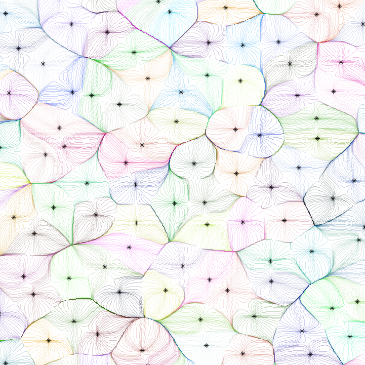
Clearly, we have no long-range order that manifests itself as non-trivial Bragg peaks, and also none that would lead to singular continuous components. Yet, there are lots of remarkable patterns that almost repeat (at random locations, of course), and one might wonder to what extent spectral theory is able to capture such features. This might be an interesting point for future investigations.
Acknowledgements
We thank Manjunath Krishnapur for drawing our attention to Gaussian analytic functions. We also thank the reviewers for their useful comments. This project was supported by the German Research Foundation (DFG), within the CRC 701. Robert V. Moody was also supported by the Natural Sciences and Engineering Research Council of Canada.
References
- [1] Abramowitz, M.; Stegun, I. A.: Handbook of Mathematical Functions. Dover Publications (1972), New York.
- [2] Anderson, G.; Guionnet, A.; Zeitouni, O.: An Introduction to Random Matrices. Cambridge University Press (2010), Cambridge.
- [3] Baake, M.; Birkner, M.; Moody, R. V.: Diffraction of stochastic point sets: explicitly computable examples. Commun. Math. Phys. 293 (2010), 611–660. arXiv:0803.1266
- [4] Baake, M.; Grimm, U.: Aperiodic Order. Volume 1: A Mathematical Invitation. Cambridge University Press (2013), Cambridge.
- [5] Baake, M.; Höffe, M.: Diffraction of random tilings: some rigorous results. J. Stat. Phys. 99 (2000), 219–261. arXiv:math-ph/9901008
- [6] Baake, M.; Kösters, H.: Random point sets and their diffraction. Philos. Mag. 91 (2011), 2671–2679. arXiv:1007.3084
- [7] Baake, M.; Lenz, D.; van Enter, A.: Dynamical versus diffraction spectrum for structures with finite local complexity. arXiv:1307.7518
- [8] Berg, C., Forst, G.: Potential Theory on Locally Compact Abelian Groups. Springer (1975), Berlin.
- [9] Cornfeld, I. P.; Fomin, S. V.; Sinai, Ya. G.: Ergodic Theory. Springer (1982), New York.
- [10] Daley, D. J.; Vere-Jones, D.: An Introduction to the Theory of Point Processes. Volume I: Elementary Theory and Methods, 2nd edition. Springer (2003), New York.
- [11] Daley, D. J.; Vere-Jones, D.: An Introduction to the Theory of Point Processes. Volume II: General Theory and Structure, 2nd edition. Springer (2008), New York.
- [12] Goueré, J.-B.: Diffraction and Palm measure of point processes. Comptes Rendus Acad. Sci. 342 (2003), 141–146. arXiv:math/0208064
- [13] Hough, J. B.; Krishnapur, M.; Peres, Y.; Virag, B.: Zeros of Gaussian Analytic Functions and Determinantal Point Processes. American Mathematical Society (2009), Providence, RI.
- [14] Lavancier, F.; Møller, J; Rubak, E.: Statistical aspects of determinantal point processes. arXiv:1205.4818
- [15] Lenz, D.; Strungaru, N.: Pure point spectrum for measure dynamical systems on locally compact abelian groups. J. Math. Pures Appl. 92 (2009), 323–341. arXiv:0704.2489
- [16] Macchi, O.: The coincidence approach to stochastic point processes. Adv. Appl. Probab. 7 (1975), 83–122.
- [17] Queffélec, M.: Substitution Dynamical Systems – Spectral Analysis, 2nd edition. Springer (2010), Berlin.
- [18] Sodin, M.; Tsirelson, B. Random complex zeros II. Perturbed lattice. Israel J. Math. 152 (2006), 105–124. arXiv:math/0309449
- [19] Soshnikov, A.: Determinantal random point fields. Russian Math. Surveys 55 (2000), 923–975. arXiv:math/0002099