Random Pairwise Gossip on $CAT(\kappa)$ Metric Spaces

Assume $V$ is some finite set. We denote by $\mathcal{P}_{2}(V)$ the set of pairs of elements in $V$: $\mathcal{P}_{2}(V)=\{\{v,w\}:v\not=w\}$. Notice that, by definition, for $v\not=w$, $\{v,w\}=\{w,v\}$ whereas $(v,w)\not=(w,v)$. Throughout the paper, $\mathcal{M}$ will denote a metric space, equipped with metric $d$. Associated with any subset $S\subset\mathcal{M}$, we define its diameter $\mathop{\mathrm{diam}}(S)=\sup\{d(s,s^{\prime}):s,s^{\prime}\in S\}$. We also define (closed) balls $B(x,r)=\{y\in\mathcal{M}:d(x,y)\leq r\}$. Random variables are denoted by upper-case letters (e.g., $X$, …) while their realizations are denoted by lower-case letters (e.g. $x$, …) Without any further notice, random variables are assumed to be functions from a probability space $\Omega$ equipped with its $\sigma$-field $\mathcal{F}$ and probability measure $\mathbb{P}$; $x=X(\omega)$ denotes the realization associated to $\omega\in\Omega$. For any set $S$ and any subset $A$, $\delta\{A\}$ denotes the indicator function that takes value $1$ on $A$ and $0$ otherwise.

We consider a network of $N$ agents represented by a graph $G=(V,E)$, where $V=\{1,\dots,N\}$ stands for the set of agents and $E$ denotes the set of available communication links between agents. A link $e\in E$ is given by a pair $\{v,w\}\in\mathcal{P}_{2}(V)$ where $v$ and $w$ are two distinct agents in the network that are able to communicate directly. Note that the graph is assumed undirected, meaning that whenever agent $v$ is able to communicate with agent $w$, the reciprocal communication is also assumed feasible. This assumption makes sense when communication speed is fast compared to agents movements speed. When a communication link $e=\{v,w\}$ exists between two agents, both agents are said to be neighbors and the link is denoted $v\sim w$. We denote by $\mathcal{N}(v)$ the set of all neighbors of the agent $v\in V$. The number of elements in $\mathcal{N}(v)$ is referred to as the degree of $v$ and denoted $\deg(v)$. The graph is assumed to be connected, which means that for every two agents $u,v$ there exists a finite sequence of agents $w_{0}=u,\dots,w_{d}=v$ such that:

This means that each two agents are at least indirectly related.

As in [BGPS06], we assume that the time model is asynchronous, i.e. that each agent has its own Poisson clock that ticks with a common intensity $\lambda$ (the clocks are identically made), and moreover, each clock is independent from the other clocks. When an agent clock ticks, the agent is able to perform some computations and wake up some neighboring agents. This time model has the same probability distribution than a global single clock ticking with intensity $N\lambda$ and selecting uniformly randomly a single agent at each tick. This equivalence is described, e.g. in [BGPS06]. From now on, we represent time by the set of integers: for such an integer $k$, time $k$ stands for the time at which the $k^{\textrm{th}}$ event occurred.

At a given time $k$, we denote by $V_{k}$ the agent whose clock ticked and by $W_{k}$ the neighbor that was in turn awaken. Therefore, at time $k$, the only communicating agents in the whole network are $V_{k}$ and $W_{k}$. A single link is then active at each time, hence, at a given time, most links are not used. We assume that $(V_{k},W_{k})$ are independent and identically distributed and that the distribution of $V_{k}$ is uniform over the network while the distribution of $W_{k}$ is uniform in the neighborhood of $V_{k}$. More precisely, the probability distribution of $(V_{k},W_{k})$ is given by:

Notice that this probability is not symmetric in $(v,w)$. It is going to turn out convenient to also consider directly the link $\{V_{k},W_{k}\}$, forgetting which node was the first to wake up and which node was second. In this case $\mathbb{P}[\{V_{k},W_{k}\}=\{v,w\}]$ is of course symmetric in $(v,w)$. One has:

The communication framework considered here is standard [BGPS06].

Each node $v\in V$ stores data represented as an element $x_{v}$ belonging to some space $\mathcal{M}$. More restrictive assumptions on $\mathcal{M}$ will follow (see section A). Initially each node $v$ has a value $x_{v}(0)$ and $X_{0}=(x_{1}(0),\dots,x_{N}(0))$ is the tuple of initial values of the network. We focus on iterative algorithms that tend to drive the network to a consensus state; meaning a state of the form $X_{\infty}=(x_{\infty},\dots,x_{\infty})$ with: $x_{\infty}\in\mathcal{M}$. We denote by $x_{v}(k)$ the value stored by the agent $v\in V$ at the $k$-th iteration of the algorithm, and $X_{k}=(x_{1}(k),\dots,x_{N}(k))$ the global state of the network at instant $k$. The general scheme is as follows: network is in some state $X_{k-1}$; agents $V_{k}$ and $W_{k}$ wake up, communicate and perform some computation to lead the network to state $X_{k}$.

In this subsection we make the following assumption.

We now define the disagreement function.

Function $\Delta$ measures how much disagreement is left in the network. Indeed, since the network is connected, $\Delta$ is $0$ if and only if the network is at consensus. It would be a graph Laplacian in the Euclidean setting. The normalizing term involving degrees gives less weight to more connected vertices, since they are more likely to be solicited by neighbors; in order to give equal weight to each edge in the graph. This normalization will turn out to be convenient in the analysis. Another important function is the variance function.

The next proposition measures the average decrease of variance at each iteration.

We now state a first convergence result.

Actually the previous proof can be adapted to give information on the convergence speed of the algorithm. Let us first prove an elementary lemma.

We are now in a position to prove the following result:

We now turn to the case of positively curved spaces.

In this section, we replace Assumption 2 by the following:

By proposition 10 we are ensured that Algorithm Random Pairwise Midpoint is well-defined. Indeed, by convexity of balls with radius smaller than $r_{\kappa}$ points will remain within distance less than $r_{\kappa}$ of each other. Moreover midpoints are well-defined and unique since $r_{\kappa}<D_{\kappa}$.

The trick used to study $CAT(\kappa)$ configurations is to replace distance $d(x,y)$ by: $\chi_{\kappa}(d(x,y))$ with $\chi_{\kappa}=1-C_{\kappa}$ being pointwise nonnegative. We adapt the definitions used in the $CAT(0)$ setting as follows:

One can remark that for all $k\geq 0$, $(v,w)\in V^{2}$: $\sigma_{\kappa}^{2}(X_{k})\geq 0$ and $\Delta_{\kappa}(X_{k})\geq 0$. Notice that $\sigma_{\kappa}^{2}(x)=0$ implies that for all $\{v,w\}\in\mathcal{P}_{2}(V)$: $\chi_{\kappa}(d(v,w))=0$; and, since $0\leq d(v,w)\leq\frac{\pi}{2\sqrt{\kappa}}$, it implies that $d(v,w)=0$, hence the system is in a consensus state. Moreover, when $\kappa\to 0$, $\Delta_{\kappa}\to\Delta$ and $\sigma^{2}_{\kappa}\to\sigma^{2}$.

The following proposition is a direct consequence of lemma 3.

With this result it is now possible to prove using the same reasoning as in proposition 1. The techniques are the same but the details differ slightly. For the sake of completeness, we give the details below.

In order to derive a convergence result we need an analogous result to Proposition 2 for $CAT(\kappa)$ spaces.

All the tools to show almost-sure convergence and speed are in place. The proofs of the following two results are exactly the same than in the $CAT(0)$ case, provided $\Delta$ and $\sigma$ are replaced by $\Delta_{\kappa}$ and $\sigma_{\kappa}$.

These results show that – provided all the initial points are close enough from each other, this is detailed by Assumption 3.3 – the situation is the same as in nonpositive curvature, namely, almost sure convergence taking place at least exponentially fast. Notice that, by contrast, there are no constraints on the initialization, for the result to hold true in $CAT(0)$. Notice also that the radius involved in Assumption 3.3 depends on the curvature upper bound $\kappa$ and ensures convexity of corresponding balls. It gives a hint that convexity plays an important role in the behavior of the algorithm, which is not surprising, since the algorithm basically amounts to take random midpoints.

The scenario in this experiment is the following. Each sensor in a network estimates a covariance matrix for some observed multivariate process. Then the network seeks a consensus on these covariance matrices. We implemented the proposed algorithm using known facts from the geometry of positive definite matrices $\mathrm{Pos}(n)$, [Lan99, chap. 12]. $\mathrm{Pos}(n)$ is equipped with distance

and

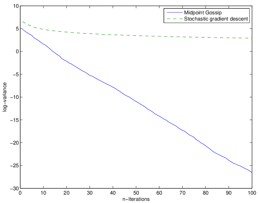
Using this distance, which comes from a Riemannian metric, $\mathrm{Pos}(n)$ is a Hadamard manifold [Lan99, p.326], see also [Bar13] for an in-depth presentation, and as such, it is a $CAT(0)$ space[Lan99, prop 3.4, p.311]. Using the previous relations, it is straightforward to implement the Midpoint Gossip algorithm and compute $\log\sigma^{2}\big(M(n)\big)$ at each iteration $n$; where $M(n)=(M_{1}(n),\dots,M_{N}(n))$ denotes the tuple of positive definite matrix held by the agents $1\leq v\leq N$ at time $n$. Regarding the initialization step, we generate $N$ iid matrices $M_{v}(0)$, following a Wishart distribution on $q\times q$ positive definite matrices with parameters $(q,1)$, i.e., as $\sum_{k=1}^{q}X_{k,v}X_{k,v}^{T}$ where $X_{k,v}\sim\mathcal{N}(0,I_{q})$ are independent standard multivariate Gaussian vectors of dimension $q$ (in this numerical experiment $q=3$ and $N=30$). Regarding the network, we experiment with both the complete graph $K_{N}$ and the path graph $P_{N}$ ($V=\{1\dots N\}$, $\{i,i+1\}\in E$ for $i\in\{1,\dots N-1\}$). The complete graph mixes information fast, while the path graph does not. It is interesting to compare the results obtained in both cases. are displayed in Figure 1 (for complete graph) and 2 (for path graph). Note that the algorithm is very close to the one proposed in [Bon13] which consists in the iterations $M^{1/2}(M^{-1/2}NM^{-1/2})^{\gamma_{n}}M^{1/2}$ where $\gamma_{n}$ is a sequence of stepsize such that $\sum_{n}\gamma_{n}=+\infty$ and $\sum_{n}\gamma_{n}^{2}<\infty$. In particular, stepsize $\gamma_{n}$ should go to $0$ while in our case it is kept constant at $1/2$. The full and dashed curves in figure 5 represent the function $\log(\sigma^{2}_{n})$ for respectively the stochastic gradient descent method (implemented with a decreasing step size $\gamma_{n}=\frac{1}{n}$) and midpoint gossip algorithm; the initialization and graph used for both algorithms being the same (complete graph), the two curves can be compared so as to deduce that while the consensus midpoint algorithm leads to exponential convergence, the $\log(\sigma^{2}_{n})$ curve for the gradient descent method seems to converge slower. Actually the fact that it converges slower is coherent with stochastic approximation with decreasing stepsize. Indeed, it is known that, in the Euclidean setting [KY97, chap. 10], for stepsize $\gamma_{n}$, the speed of convergence is of order ${\gamma_{n}}^{-1/2}$.

It is also interesting in this case to make a comparison for positive definite matrices between the Midpoint gossip algorithm and the Euclidean arithmetic gossip. In figure 3 we plot $n\mapsto\sigma^{2}_{n}$ where $n$ is the number of iterations and $\sigma^{2}$ is the sum of ”non Euclidean” distances squared. The result suggests that the Arithmetic gossip algorithm has a slight advantage over midpoint gossip in terms of convergence speed. However, if we plot $n\mapsto\sigma^{2}_{n,E}$ where $\sigma^{2}_{n,E}=\frac{1}{N}\sum_{\{i,j\}\in\mathcal{P}_{2}(V)}||x_{i}(n)-x_{j}(n)||_{F}^{2}$ and $||.||_{F}$ is the Frobenius Euclidean norm, the opposite seems to be true, as shown in figure 4 midpoint algorithm performs slightly better. The midpoint gossip algorithm converges faster than arithmetic gossip when the variance is expressed in Euclidean distances.

Consider a network $G=(V,E)$ of robotic arms capable of performing two types of rotations $R_{1}$ and $R_{2}$, of distinct rotation axes $\Delta_{1}$ and $\Delta_{2}$. After being assigned an axis of rotation, an arm rotates continuously around that axis until it reaches its target rotation angle or gets interrupted. At an initial time, all arms are in an identical position. After that they evolve separately. To recollect them in a common position, they unwind all their movements, provided they kept the whole history. Here, we argue that a less costly procedure could be applied. We apply Algorithm Random Pairwise Midpoint on a convenient state space that we describe below, to drive the arms near a consensus position, in a completely distributed and autonomous fashion.

We assume furthermore that $R_{1}$ and $R_{2}$ are chosen in “generic position”. By that, we mean that they are realizations of independent and uniform random variables on $SO_{3}$ (i.e. according to the Haar measure on $SO_{3}\times SO_{3}$). As such, it is known, [Eps71], that they are almost surely algebraically independent, i.e., if $\exists n>0$, $(k_{1},\dots,k_{n})\in\{-1,1\}$ and $i_{1}\dots i_{n}\in\{1,2\}$ such that: $R_{i_{1}}^{k_{1}}R_{i_{2}}^{k_{2}}\dots R_{i_{n}}^{k_{n}}=I$, then there exists two consecutive indices $i_{j}$, $i_{j+1}$ such that $i_{j}=i_{j+1}$.

Define the set of words $\mathcal{A}^{*}$ on alphabet $\mathcal{A}=\{a,a^{-1},b,b^{-1}\}$ and the set of admissible words $\mathcal{A}^{*}_{0}$ such that no two consecutive letters are inverse from each other. Map letter $a$ to $R_{1}$, $a^{-1}$ to $R_{1}^{-1}$, letter $b$ to $R_{2}$ and $b^{-1}$ to $R_{2}^{-1}$. The concatenation of words is mapped to the product of corresponding rotations. We refer to this mapping as $\varphi:\mathcal{A}_{0}^{*}\to SO_{3}$. For instance $\varphi(bab^{-1}a)=R_{2}R_{1}R_{2}^{-1}R_{1}$. Since, $R_{1}$ and $R_{2}$ are algebraically independent, map $\varphi$ is injective. Consider the directed Cayley graph $\mathcal{G}$ with vertices $\mathcal{V}=\mathcal{A}^{*}_{0}$ , edges set $E$ defined as:

Define the endpoint maps $\partial_{0}$ and $\partial_{1}$ $:E\to\mathcal{V}$ such that $\partial_{0}(e)=w$ and $\partial_{1}(e)=w^{\prime}$ for $e=(w,w^{\prime})\in E$. Equipped with its endpoint maps, $\mathcal{G}$ is called a combinatorial graph. To turn $\mathcal{G}$ into a metric graph, we follow a standard construction, see, e.g. [BH99, p.7]. Let us form the quotient set $X_{\mathcal{G}}=E\times[0,1]/\sim$ where the equivalence relation $\sim$ is such that $(e,i)\sim(e^{\prime},i^{\prime})$ iff $\partial_{i}(e)=\partial_{i^{\prime}}(e^{\prime})$, with $i,i^{\prime}\in\{0,1\}$. We adopt the convention to choose $(e,1)$ to represent the equivalence class $\{(e,1),(e^{\prime},0)\}$ when $\partial_{0}(e^{\prime})=\partial_{1}(e)$. We then equip $X_{\mathcal{G}}$ with the standard metric distance $d_{X}$, as described, e.g. in [BH99, p.7].

References

- [Bar13] Frédéric Barbaresco. Information geometry of covariance matrix: Cartan-Siegel homogeneous bounded domains, Mostow/Berger fibration and Frechet median. In Matrix Information Geometry, pages 199–255. Springer, 2013.
- [BGPS06] Stephen Boyd, Arpita Ghosh, Balaji Prabhakar, and Devavrat Shah. ”Randomized gossip algorithms”. IEEE Trans. Inf. Theory, 52(6):2508–2530, Jun 2006.
- [BH99] Martin Bridson and André Haefliger. Metric Spaces of Non-Positive Curvature. Springer Verlag, 1999.
- [Bon13] Silvère Bonnabel. ”Stochastic gradient descent on Riemannian manifolds”. IEEE Trans. Autom. Control, 58(9):2217–2229, Sep 2013.
- [Bur06] Mike Burrows. ”The chubby lock service for loosely-coupled distributed systems”. In Proceedings of the 7th symposium on Op. sys. design and implem., pages 335–350, 2006.
- [Cha06] Issac Chavel. Riemannian Geometry. Cambridge University Press, second edition, 2006.
- [DC92] Manfredo Do Carmo. Riemannian Geometry. Birkhäuser, 1992.
- [Eps71] David Epstein. Almost all subgroups of a lie group are free. Journal of Algebra, 19(2):261–262, 1971.
- [KY97] Harold Kushner and George Yin. Stochastic Approximation Algorithms and Applications. Springer, 1997.
- [Lan99] Serge Lang. Fundamentals of Differential Geometry. Springer, 1999.
- [SG07] Luca Schenato and Giovanni Gamba. ”A distributed consensus protocol for clock synchronization in wireless sensor network”. In IEEE Conf on Decision and Control, pages 2289–2294, 2007.
- [SRG08] Ioannis Schizas, Alejandro Ribeiro, and Georgios Giannakis. ”Consensus in ad hoc WSNs with noisy links—part I: Distributed estimation of deterministic signals”. IEEE Trans. Signal Process, 56(1):350–364, Jan 2008.
- [SS09] Alain Sarlette and Rodolphe Sepulchre. ”Consensus optimization on manifolds”. SIAM Journal on Control and Optimization, 48(1):56–76, 2009.
- [TAV13] Roberto Tron, Bijan Afsari, and René Vidal. ”Riemannian consensus for manifolds with bounded curvature”. IEEE Trans. Autom. Control, 58(4):921–934, 2013.
- [TVT08] Roberto Tron, René Vidal, and Andreas Terzis. ”Distributed pose averaging in camera networks via consensus on SE(3)”. In Second ACM/IEEE International Conference on Distributed Smart Cameras. ICDSC, pages 1–10, 2008.