Spatial Spectrum Access Game
Abstract
A key feature of wireless communications is the spatial reuse. However, the spatial aspect is not yet well understood for the purpose of designing efficient spectrum sharing mechanisms. In this paper, we propose a framework of spatial spectrum access games on directed interference graphs, which can model quite general interference relationship with spatial reuse in wireless networks. We show that a pure Nash equilibrium exists for the two classes of games: (1) any spatial spectrum access games on directed acyclic graphs, and (2) any games satisfying the congestion property on directed trees and directed forests. Under mild technical conditions, the spatial spectrum access games with random backoff and Aloha channel contention mechanisms on undirected graphs also have a pure Nash equilibrium. We also quantify the price of anarchy of the spatial spectrum access game. We then propose a distributed learning algorithm, which only utilizes users’ local observations to adaptively adjust the spectrum access strategies. We show that the distributed learning algorithm can converge to an approximate mixed-strategy Nash equilibrium for any spatial spectrum access games. Numerical results demonstrate that the distributed learning algorithm achieves up to performance improvement over a random access algorithm.
I Introduction
Cognitive radio is envisioned as a promising technology to alleviate the problem of spectrum under-utilization [2]. It enables unlicensed wireless users (secondary users) to opportunistically access the licensed channels owned by legacy spectrum holders (primary users), and thus can significantly improve the spectrum efficiency [2].
A key challenge of the cognitive radio technology is how to resolve the resource competition by selfish secondary users in a decentralized fashion. If multiple secondary users transmit over the same channel simultaneously, severe interferences or collisions might occur and the individual as well as total data rates of all users may get reduced. Therefore, it is necessary to design efficient spectrum sharing mechanisms for cognitive radio networks.
The competitions among secondary users for common spectrum have often been studied as a noncooperative game (e.g., [3, 4, 5, 6] and the references therein). For example, Nie and Comaniciu in [4] designed a self-enforcing distributed spectrum access mechanism based on potential games. Niyato and Hossain in [5] studied a price-based spectrum access mechanism for competitive secondary users. F¨¦legyh¨¢zi et al. in [6] proposed a two-tier game framework for medium access control (MAC) mechanism design.
When not knowing the spectrum information such as channel availability, secondary users need to learn the network environment and adapt the spectrum access decisions accordingly. Han et al. in [7] used the no-regret learning to solve this problem, assuming that the users’ channel selections are common information. When users’ channel selections are not observable, Anandkumar et al. in [8] as well as Liu and Zhao in [9] designed multi-agent multi-armed bandit learning algorithms to minimize the expected performance loss of distributed spectrum access.
A common assumption of the above studies is that secondary users are close-by and interfere with each other when they transmit on the same channel simultaneously. However, a unique feature of wireless communication is spatial reuse. If users who transmit simultaneously are located sufficiently far away, then simultaneous transmissions over the same channel may not cause any performance degradation to the users. Such spatial effect on spectrum sharing is less understood than many other aspects in the existing literature [10].

Recently, Tekin et al. in [11] proposed a novel spatial congestion game framework to take spatial relationship into account. The key idea is to extend the classical congestion game upon an undirected graph, by assuming that the interferences among the players are symmetric and a player’s throughput depends on the number of players in its neighborhood that choose the same resource. However, the interference relationship among the secondary users can be asymmetric due to the heterogeneous transmission powers and locations of the users. We hence propose a more general framework of spatial spectrum access game on directed interference graphs, which take users’ heterogeneous resource competition capabilities and asymmetric interference relationship into account. The congestion game on directed graphs has also been studied in [12], with the assumption that players have linear and homogeneous payoff functions. The game model in this paper is more general and allows both linear and nonlinear player-specific payoff functions. Moreover, we design a distributed algorithm for achieving the equilibria of the game. The main results and contributions of this paper are as follows:
- •
General game formulation: We formulate the distributed spectrum access problem as a spatial spectrum access game on directed interference graphs, with user-specific channel data rates and channel contention capabilities.
- •
Existence of Nash equilibria: We show by counter examples that a general spatial spectrum access game may not have a pure Nash equilibrium. We then show that a pure strategy equilibrium exists in the following two classes of games: (1) any spatial spectrum access games on directed acyclic graphs, and (2) any games satisfying the congestion property on directed trees and directed forests. We also show that under mild conditions the spatial spectrum access games with random backoff and Aloha channel contention mechanisms on undirected graphs are potential games and have pure Nash equilibria. We also quantify the price of anarchy of the spatial spectrum access game.
- •
Distributed learning for achieving an approximate Nash equilibrium: We develop a maximum likelihood estimation approach for estimating user expected throughput based on local observations. Based on the local estimation of user expected throughputs, we then propose a distributed learning algorithm that can converge to an approximate mixed Nash equilibrium for any spatial spectrum access games. Numerical results demonstrate that the distributed learning algorithm achieves up-to performance improvement over the random access algorithm.
Due the space limit, all the proofs in this paper can be found in the supplementary file on the TMC website or the online technical report in [13].
II System Model
We consider a cognitive radio network with a set of independent and stochastically heterogeneous primary channels. A set of secondary users try to access these channels distributively when the channels are not occupied by primary (licensed) transmissions. Here we assume that each secondary user is a dedicated transmitter-receiver pair.
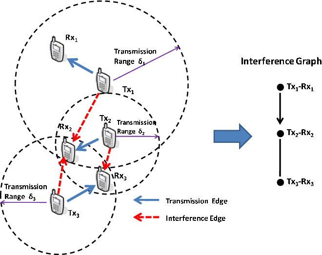
To take users’ spatial relationship into account, we denote as the location vector of secondary user , where and denote the location of the transmitter and the receiver, respectively. Each secondary user has a interference range . Then given the location vectors of all secondary users, we can obtain the interference graph to describe the interference relationship among the users. Here the vertex set is the same as the secondary user set. The edge set is defined as , where is the distance between the transmitter of user and the receiver of user . In general, an interference edge can be directed or undirected. If an interference edge is directed from secondary user to user , then user ’s data transmission will be affected by user ’s transmission on the same channel, but user will not be affected by user . If the interference edge is undirected11 1 Here the edge is actually bi-directed. We follow the conventions in [11] and ignore the directions on the edge. between user and user , then the two users can affect each other. Note that a generic directed interference graph can consist of a mixture of directed and undirected edges. In the sequel, we call an interference graph undirected, if and only if all the edges of the graph are undirected. We also denote the set of users that can cause interference to user as .
Based on the interference model above, we describe the cognitive radio network with a slotted transmission structure as follows:
- •
Channel State: the channel state for a channel during time slot is if channel is occupied by primary transmissions and otherwise.
- •
Channel State Transition: for a channel , the channel state is a random variable with a probability density function as . In the following, we denote the channel idle probability as the mean of , i.e., . For example, the state of a channel changes according to a two-state Markovian process. We denote the channel state probability vector of channel at time as which forms a Markov chain as with the transition matrix
Furthermore, the long run statistical channel availability of a channel can be obtained from the stationary distribution of the Markov chain, i.e.,
(1) As another example, we can also use the channel idle probability to indicate the spectrum availability for white-space spectrum access. Due to the fact that the activities of primary users on TV channels typically change very slowly, the most recent FCC ruling requires white-space devices (i.e., secondary users of TV channels) to determine the spectrum availability via a database [14]. In this case, we can set that if the TV channel is vacant for secondary users and otherwise.
- •
User Specific Channel Throughput: for each secondary user , its realized data rate on an idle channel in each time slot evolves according to a random process with a mean , due to users’ heterogeneous transmission technologies and the local environmental effects such as fading. For example, we can compute the data rate according to the Shannon capacity as
(2) where is the channel bandwidth, is the fixed transmission power adopted by user according to the requirements such as the primary user protection, denotes the background noise power, and is the channel gain. In a Rayleigh fading channel environment, the channel gain is a realization of a random variable that follows the exponential distribution.
- •
Time Slot Structure: each secondary user executes the following stages synchronously during each time slot:
- –
Channel Sensing: sense one of the channels based on the channel selection decision made at the end of previous time slot.
- –
Channel Contention: Let be the channel selected by user , and be the channel selection profile of all users. The probability that user can grab the chosen idle channel during a time slot is , which depends on the subset of user ’s interfering users that choose the same channel . Here are two examples:
1) Random backoff mechanism: the contention stage of a time slot is divided into mini-slots22 2 The contention window size plays an important role for optimizing the system performance. If is too small, it would increase the collision probability among users and hence negatively affect the system performance. In general, if is too large, it would reduce the spectrum access time and hence reduce the system throughput. To optimize the system performance, we can adopt the approach in [15] to determine the optimal contention window size.. Each contending user first counts down according to a randomly and uniformly generated integer backoff time counter (number of mini-slots) between and . If there is no active transmissions till the count-down timer expires, the user monitors the channel and transmits RTS/CTS messages on that channel. If multiple users choose the same backoff counter, a collision will occur and no users can grab the channel successfully. Once successfully gets the channel, the user starts to transmit its data packet. In this case, we have(3) where denotes the number of user ’s interfering users choosing the same channel as user .
2) Aloha mechanism: user contends for an idle channel with a probability in a time slot. If multiple interfering users contend for the same channel, a collision occurs and no user can grab the channel for data transmission. In this case, we have(4) - –
Data Transmission: transmit data packets if the user successfully grabs the channel.
- –
Channel Selection: choose a channel to access during next time slot according to the distributed learning algorithm in Section VI.
- –
Under a fixed channel selection profile , the long-run average throughput of a secondary user choosing channel can be computed as
| (5) |
Note that in practices, due to hardware constraint each secondary user typically cannot observe the channel states of all the channels in each time slot. In this case, one possible modeling approach is to formulate the distributed spectrum access problem as a partial-observation dynamic game, such that the game state is defined as the channel states in the current time slot, and each secondary user has a partial observation of the game state in each time slot. However, it is well-known that such a partial-observation dynamic game is very difficult to analyze, and is computationally intractable due to the curse of dimensionality. To enable tractable analysis and achieve an efficient spectrum access, we hence study the distributed spectrum access problem from the long-run average perspective, and utilize the statistical channel availability information (i.e., channel idle probability ) to aid secondary users’ decisions makings. This is because that the statistical channel availability information can be learned from the history of a secondary user’s local observations, via the maximum likelihood estimation approach described in Section VI. Moreover, the spatial spectrum access game solution in this paper can help us solve the complete information dynamic game, where each secondary user is able to globally observe the channel state realization of all the channels in each time slot. Since the secondary users cannot control the transition of channel states, we can easily derive the solution of the complete information dynamic game as follow: for each time slot , we solve the corresponding stage spatial spectrum access game using the algorithm proposed in this paper, with the channel idle probabilities of the stage game replaced by the channel state realization of time slot . Since our analysis is from the secondary users’ perspective, we will use the terms “secondary user” and “user” interchangeably.
III Spatial Spectrum Access Game
We now consider the problem that each user tries to maximize its own throughput by choosing a proper channel distributively. Let be the channels chosen by all other users except user . Given other users’ channel selections , the problem faced by a user is
| (6) |
The distributed nature of the channel selection problem naturally leads to a formulation based on the game theory, such that users can self organize into a mutually acceptable channel selection (pure Nash equilibrium) with
| (7) |
We thus formulate the distributed channel selection problem on an interference graph as a spatial spectrum access game , where is the set of players, is the set of strategies, describes the interference relationship among the players, and is the payoff function of player .
It is known that not every finite strategic game possesses a pure Nash equilibrium [16]. We then introduce a more general concept of mixed Nash equilibrium. Let denote the mixed strategy of user , where is the probability of user choosing channel , and . For simplicity, we use the same payoff notation to denote the expected throughput of user under the mixed strategy profile , and it can be computed as
| (8) |
Similarly to the pure Nash equilibrium, the mixed Nash equilibrium is defined as:
Definition 1 (Mixed Nash Equilibrium [16]).
The mixed strategy profile is a mixed Nash equilibrium, if for every user , we have
where denote the mixed strategy choices of all other users except user .
One important property deduced from the mixed Nash equilibrium definition is that if a user assigns some positive probabilities of choosing some actions, then the expected payoff of these actions should be the same at the equilibrium. Otherwise, the user can improve by increasing the probability of choosing the action with higher expected payoff. In the spatial spectrum access game, each secondary user takes both the primary activity levels on different channels and the competition with other secondary users into consideration, in order to improve its long run average throughput. Nash equilibrium is the natural solution concept for the spatial spectrum access game. At a Nash equilibrium, secondary users are mutually satisfied with their long run average throughputs and no user can improve by changing its channel unilaterally.
In the following sections, we will study the existence of both mixed and pure Nash equilibria based on the global network information, and then discuss how to achieve the Nash equilibria based on the local user observations only.
IV Existence of Nash Equilibria
In this part, we study the existence of Nash equilibria in a spatial spectrum access game. Since a spatial spectrum access game is a finite strategic game (i.e., with finite number of players and finite number of channels), we know that it always admits a mixed Nash equilibrium according to [16].
On the other hand, not every finite strategic game possesses a pure Nash equilibrium [16]. Compared with mixed Nash equilibrium, Pure Nash equilibrium can achieve the mutually satisfactory spectrum sharing solution without requiring the frequent channel switching and hence helps to reduce the system overhead such as energy consumption of frequent channel switching. This motivates us to further investigate the existence of pure Nash Equilibria of the spatial spectrum access games.
IV-A Existence of Pure Nash Equilibria on Directed Interference Graphs
We first study the existence of pure Nash Equilibria on directed interference graphs.
First of all, we can construct a game which does not have a pure Nash equilibrium.
Theorem 1.
There exists a spatial spectrum access game on a directed interference graph not admitting any pure Nash equilibrium.
Figure 3 shows such an example. It is easy to verify that for all possible channel selection profiles, there always exists one user (out of these three users) having an incentive to change its channel selection unilaterally to improve its throughput.

We then focus on identifying the conditions under which the game admits a pure Nash equilibrium. To proceed, we first introduce the following lemma (the proof is given in the appendix in the separate supplemental file).
Lemma 1.
Assume that any spatial spectrum access game with users on a given directed interference graph has a pure Nash equilibrium. Then we can construct a new spatial spectrum access game by adding a new player, who can not generate interference to any player in the original game and may receive interference from one or multiple players in the original game. The new game with users also has a pure Nash equilibrium.
We know that any directed acyclic graph (i.e., a directed graph contains no directed cycles) can be given a topological sort (i.e., an ordering of the nodes), such that if node then there are no edges directed from the node to node in the ordering [17]. This is due to that any spatial spectrum access game with user always has a pure Nash equilibrium. By the induction argument, we know from Lemma 1 that
Corollary 1.
Any spatial spectrum access game on a directed acyclic graph has a pure Nash equilibrium.
To obtain more insightful results, we next impose the following property on the spatial spectrum access games:
Definition 2 (Congestion Property).
User ’s channel grabbing probability satisfies the congestion property if for any , we have
| (9) |
Furthermore, a spatial spectrum access game satisfies the congestion property if (9) holds for all users
The congestion property (CP) means that the more contending users exist, the less chance a user can grab the channel. Such a property is natural for practical wireless systems such as the random backoff and Aloha systems. We can show that the following result (the proof is given in the appendix in the separate supplemental file).
Lemma 2.
Assume that any spatial spectrum access game with users satisfying the congestion property on a given directed interference graph has a pure Nash equilibrium. Then we can construct a new spatial spectrum access game by adding a new player, whose channel grabbing probability satisfies the congestion property and who has an interference relationship with at most one player in the original game. The new game with users also has a pure Nash equilibrium.
Definition 3 (Directed Tree [17]).
A directed graph is called a directed tree if the corresponding undirected graph obtained by ignoring the directions on the edges of the original directed graph is a tree.
Note that a (undirected) tree is a special case of directed trees. Since any spatial spectrum access game over a single node always has a pure Nash equilibrium, we can then construct the directed tree recursively by introducing a new node and adding an (directed or undirected) edge between this node and one existing node. By the induction argument, we obtain from Lemma 2 that
Corollary 2.
Any spatial spectrum access game satisfying the congestion property on a directed tree has a pure Nash equilibrium.
Definition 4 (Directed Forest [17]).
A directed graph is called a directed forest if it consists of a disjoint union of directed trees.
Similarly, we can obtain from Lemma 2 that
Corollary 3.
Any spatial spectrum access game satisfying the congestion property on a directed forest has a pure Nash equilibrium.

Note that directed acyclic graph and directed tree structures are widely observed in many wireless networking systems such as wireless ad hoc and sensor networks [18]. For example, the star topology with sink/hub nodes in wireless sensor networks is a special case of directed tree. Based on Lemmas 1 and 2, we can construct more general directed interference graphs over which a spatial spectrum access game satisfying the congestion property has a pure Nash equilibrium. Figure 4 illustrates such an example.
IV-B Existence of Pure Nash Equilibria on Undirected Interference Graphs
We now study the case that the interference graph is undirected. This is a good approximation of reality if the transmitter of each user is close to its receiver, and all users’ interference ranges are roughly the same. For example, in 802.11 systems, undirected interference graph is widely used to approximate the interference relationships since the access points are typically close to their associated clients and the carrier sensing ranges are similar.
When an undirected interference graph is a tree, according to Corollary 2, any spatial spectrum access game satisfying the congestion property has a pure Nash equilibrium. However, for those non-tree undirected graphs without a topological sort, the existence of pure Nash equilibrium can not be proved following the results in previous Section IV-A. This motivates us to further study the existence of pure Nash equilibria on generic undirected interference graphs.
First of all, [19] showed that a -players and -resources congestion game with user-specific congestion weights may not have a pure Nash equilibrium. Such a congestion game can be considered as a spatial spectrum access game on a complete undirected interference graph (by regarding the resources as channels). When all users have homogeneous channel contention capabilities and all channels have the same mean data rates, [11] showed that the spatial spectrum access game on any undirected interference graphs has a pure Nash equilibrium. Clearly, the applicability of such a channel-homogeneous model is quite limited, since the channel throughputs in practical wireless networks are often heterogeneous. We hence next focus on exploring the random backoff and Aloha systems with user-specific data rates, which provide useful insights for the user-homogeneous and user-heterogeneous channel contention mechanisms, respectively.
Here we resort to a useful tool of potential game33 3 Note that it is much more difficult to find a proper potential function to take into account users’ asymmetric relationships (i.e., directions of edges on graph) when the interference graph is directed. Hence in this study we only apply the tool of potential game in the undirected case., which is defined as
Definition 5 (Potential Game [20]).
A game is called a potential game if it admits a potential function such that for every and ,
where is the sign function.
Definition 6 (Better Response Update [20]).
The event where a player changes to an action from the action is a better response update if and only if .
An appealing property of the potential game is that it always admits a pure Nash equilibrium and the finite improvement property, which is defined as
Definition 7 (Finite Improvement Property [20]).
A game has the finite improvement property if any asynchronous better response update process (i.e., no more than one player updates the strategy at any given time) terminates at a pure Nash equilibrium within a finite number of updates.
Based on the potential game theory, we first study the random backoff mechanism. We show in Theorem 2 that when the undirected interference graph is complete, there exists indeed a pure Nash equilibrium.
Theorem 2.
Any spatial spectrum access game on a complete undirected interference graph with the random backoff mechanism is a potential game with the potential function
| (10) |
where is the number of users choosing channel under the strategy profile , and hence has a pure Nash equilibrium.
The proof is similar to that in [21], and hence is omitted here. We then consider the spatial spectrum access game with the random backoff mechanism on bipartite graphs.
Definition 8 (Bipartite Graph [17]).
An undirected graph is called a bipartite graph if the set of its nodes can be decomposed into two disjoint sets, such that no two nodes within the same set are connected by an edge.
Definition 9 (Complete Bipartite Graph [17]).
An undirected graph is called a complete bipartite graph if it is a bipartite graph and any two nodes selected from the two disjoint sets respectively are connected by an edge.
Definition 10 (Regular Bipartite Graph [17]).
An undirected graph is called a regular bipartite graph if it is a bipartite graph and each node is connected by the same number of edges.
Note that a complete bipartite graph that has the same number of vertices in the two disjoint sets is also a regular bipartite graph. Many well known graphs such as star graphs, circulant graphs, cycle graphs with even number of vertexes, hypercubes, and rectangular lattices are either complete bipartite graphs or regular bipartite graphs. We consider the user specific throughput as
| (11) |
where represents as a user-specific transmission gain. We can show that
Theorem 3.
Any spatial spectrum access game on either a complete bipartite interference graph or a regular bipartite interference graph with user specific transmission gains and the random backoff mechanism has a pure Nash equilibrium.
The proof is given in the appendix in the separate supplemental file. We then consider the random backoff mechanism in the asymptotic case that goes to infinity. This can be a good approximation of reality when the number of backoff mini-slots is much greater than the number of interfering users, and collision rarely occurs. In this case, we have
| (12) |
here denotes the number of users that choose channel and can interfere with user . Equation (12) implies that the channel opportunity is equally shared among contending users (including user ). This can also apply in TDMA channel access mechanism. We consider the user specific throughput as
| (13) |
We show that
Theorem 4.
Any spatial spectrum access game on any undirected interference graph with user-specific transmission gains and the random backoff mechanism in the asymptotic case is a potential game with the potential function
| (14) |
and hence has a pure Nash equilibrium.
Theorem 4 is a direct consequence of the more general result Theorem 5. More specifically, we generalize the throughput function in (13) as
| (15) |
where denotes user specific channel sharing weight. When , the throughput function in (15) degenerates to the equal-sharing case in (13). The physical meaning of (15) is that the channel is shared among the contending users according to their weights. We refer this to the spatial spectrum access game with user specific sharing weights. Such a proportional channel sharing scheme has been widely used to model the heterogenous channel access priority assignment for heterogenous users of different QoS requirements in wireless networks [22]. We show that
Theorem 5.
Any spatial spectrum access game with user specific sharing weights on any undirected interference graph is a potential game with the potential function as
| (16) |
and hence has a pure Nash equilibrium.
The proof is given in the appendix in the separate supplemental file. We then consider the random access mechanism under the scenario where all channels are homogeneous to each user (i.e., and for all ). This models the case where a licensed spectrum band of a large bandwidth (e.g., TV channel) is divided into equal width logical channels for secondary usage with interleaving technology at the physical layer (e.g., the IEEE 802.16d/e standard), such that all channels exhibit the same primary occupancy and have the same channel gain to the same user (but still different channel gains for different users). In this case, the user throughput function is given as
| (17) |
We can show that the following result (the proof is given in the appendix in the separate supplemental file).
Theorem 6.
Any spatial spectrum access game on any undirected interference graph with homogeneous channels, user-specific transmission gains, and the random backoff mechanism is a potential game with the potential function
and hence has a pure Nash equilibrium.
We now consider the Aloha mechanism. According to (4), we have the throughput function as
| (18) |
We can show that the following result (the proof is given in the appendix in the separate supplemental file).
Theorem 7.
Any spatial spectrum access game on any undirected interference graph with the Aloha mechanism is a potential game with the potential function
and hence has a pure Nash equilibrium.
V Price of Anarchy
In previous sections, we have considered the existence of Nash equilibrium of spatial spectrum access games. We will further explore the efficiency of the Nash equilibrium.
Following the definition of price of anarchy (PoA) in game theory [23], we will quantify the efficiency ratio of the worst-case Nash equilibrium over the centralized optimal solution. Let be the set of Nash equilibria of a given spatial spectrum access game. Then the PoA is defined as
which is always not greater than . A larger PoA implies that the set of Nash equilibrium is more efficient (in the worst-case sense) using the centralized optimum as a benchmark. Let . For a general spatial spectrum access game, we have the following result.
Theorem 8.
The PoA of a spatial spectrum access game is at least .
The proof is given in the appendix in the separate supplemental file. Intuitively, Theorem 8 indicates that we can increase the efficiency of spectrum sharing by better utilizing the gain of spatial reuse (i.e., reducing the interference edges on the interference graph).
VI Distributed Learning For Spatial Spectrum Access Game
As mentioned in Section III, both pure and mixed Nash equilibria are important equilibrium concepts for spatial spectrum access games, characterizing system states where secondary users achieve a mutually satisfactory spectrum sharing solution. We hence consider how to achieve the Nash equilibrium for the spatial spectrum access games in this section.
As shown in Section IV, a generic spatial spectrum access game does not necessarily have a pure Nash equilibrium, and thus it is impossible to design a mechanism that is guaranteed to reach a pure Nash equilibrium in general. However, when the spatial spectrum access game is a potential game, a pure Nash equilibrium exists. In this case, we can apply the Safe Experimentation algorithm in [24] for achieving the pure Nash equilibrium. The key idea is to explore the pure strategy space based on the finite improvement property of the potential game. From the practical application’s perspective, we can apply the results obtained in Section IV to identify whether the spectrum sharing system satisfies the potential game property. We can then apply the Safe Experimentation algorithm to achieve the pure Nash equilibrium when the system possesses the potential game property.
Since any spatial spectrum access game always admits a mixed Nash equilibrium, we next target on approaching the mixed Nash equilibria. From a practical point of view, if the spectrum sharing system is complex and it is difficult to verify the existence of pure Nash equilibrium, we can consider to achieve a mutually satisfactory spectrum sharing solution by allowing users to choose mixed strategies. Govindan and Wilson in [25] proposed a global Newton method to compute the mixed Nash equilibria for any finite strategic games. This method hence can be applied to find the mixed Nash equilibria for the spatial spectrum access games. However, such an approach is a centralized optimization, which requires that each user has the complete information of other users and compute the solution accordingly. This is often infeasible in a cognitive radio network, since acquiring complete information requires heavy information exchange among the users, and setting up and maintaining a common control channel for message broadcasting demands high system overheads [2]. Moreover, this approach is not incentive compatible since some users may not be willing to share their local information due to the energy consumption of information broadcasting. We thus propose a distributed learning algorithm for any spatial spectrum access games, and the algorithm does not require any information exchange among users. Each user only learns to adjust its channel selection strategy adaptively based on its local throughput observations. We show that the distributed learning algorithm can converge to a mixed Nash equilibrium approximately.
VI-A Expected Throughput Estimation
For the distributed learning algorithm, we consider that each user does not have the complete network information and can only estimate its expected throughput locally. Similarly to the approaches in [26] and [27], we can divide the spectrum access time into a sequence of decision periods indexed by , where each decision period consists of time slots. During a single decision period, a user accesses the same channel in all time slots in order to better understand the environment. At the end of each decision period , a user observes , , and . Here denotes the state of the chosen channel (i.e., whether occupied by the primary traffic), indicates whether the user has successfully grabbed the channel, i.e.,
and is the received data rate on the chosen channel by user at time slot . Note that if (i.e., the channel is occupied by the primary traffic), we set and to be . At the end of each decision period , each user will have a set of local observations . Based on these observations, each user can then apply the Maximum Likelihood Estimation (MLE) method to estimate its expected throughput . As an example, we next consider the MLE of user expected throughput in the Markovian channel environment introduced in Section II.
We first consider the estimation of the channel idle probability . From the observation set at period , user can observe a sequence of channel state transitions as
Here there are four different transition types between adjacent time slots t and t+1: . We denote as the number of occurrences of the four state transitions types in , respectively. According to the principle of MLE, user can then compute the likelihood function in terms of channel state transition parameters as
Then MLE of can be computed by maximizing the log-likelihood function , i.e., . By the first order condition, we obtain the optimal solution as
According to (1), we can then estimate the channel idle probability as
We then consider the estimation of channel grabbing probability . When a channel is idle (i.e., no primary traffic), a user will contend for the channel and can successfully grab the channel with a probability . Since there are a total of rounds of channel contentions in the period and each round is independent, the total number of successful channel captures by user follows the Binomial distribution. User then computes the likelihood of as
Then MLE of can be computed by maximizing the log-likelihood function , i.e., . By the first order condition, we obtain the optimal solution as
We finally consider the estimation of mean data rate . Since the received data rate is also i.i.d. over different time slots, similar to the MLE of the channel grabbing probability , we can obtain the MLE of mean data rate as
By the MLE above, we can then estimate the true expected throughput as In the following analysis of distributed learning algorithm, we consider a general setting where the estimated expected throughput of user can be noisy. More precisely, we assume that where is the random estimation noise with a probability density function satisfying .
VI-B Distributed Learning Algorithm
Based on the expected throughput estimation, we then propose the distributed learning algorithm for spatial spectrum access games. The idea is to extend the principle of single-agent reinforcement learning to a multi-agent setting. Such multi-agent reinforcement learning algorithm has also been applied to the classical congestion games on complete interference graphs [28, 29] by assuming that users are homogeneous (i.e., user’s payoff only depends on the number of users choosing the same resource). Here we extend the learning algorithm to the generalized spatial congestion games on any generic interference graphs with heterogeneous users, which lead to significant differences in analysis. For example, we show that the convergence condition for the learning algorithm depends on the structure of spatial reuse, which is different from those results in [28, 29].
More specifically, at the beginning of each period , a user chooses a channel to access according to its mixed strategy , where is the probability of choosing channel . The mixed strategy is generated according to , which represents its perceptions of the payoff performance of choosing different channels based on local estimations. Perceptions are based on local observations in the past and may not accurately reflect the expected payoff. For example, if a user has not accessed a channel for many decision intervals, then perception can be out of date. The key challenge for the learning algorithm is to update the perceptions with proper parameters such that perceptions equal to expected payoffs at the equilibrium.
Similarly to the single-agent learning, we choose the Boltzmann distribution as the mapping from perceptions to mixed strategies, i.e.,
| (19) |
where is the temperature that controls the randomness of channel selections. When , each user will choose to access channels uniformly at random. When , user always chooses the channel with the largest perception value among all channel . We will show later on that the choice of trades off convergence and performance of the learning algorithm.
At the end of a decision period , a user estimated its expected throughput as , and adjusts its perceptions as
| (20) |
where are the smoothing factors. A user only changes the perception of the channel just accessed in the current decision period, and keeps the perceptions of other channels unchanged.
Algorithm 1 summarizes the distributed learning algorithm. We then analyze the complexity of the distributed learning algorithm. In each iteration, Line involves the arithmetic operations over channels and hence has the complexity of . The expected throughput estimation in Line typically involves the arithmetic operations based on the observations of the chosen channel in time slots of the decision period and hence has the complexity of . In Line , the perception value update is only carried out in the chosen channel and hence has the complexity of . Suppose that it takes iterations for the algorithm to converge. Then total computational complexity of the algorithm is at most .
VI-C Convergence of Distributed Learning Algorithm
We now study the convergence of the proposed distributed learning algorithm based on the theory of stochastic approximation [30].
First, the perception value update in (20) can be written in the following equivalent form,
| (21) |
where is the update value defined as
| (22) |
For the sake of brevity, we denote the perception values, update values, and mixed strategies of all the users as , , and , respectively.
Let denote the conditional probability that, given that the users’ perceptions are and user chooses channel , the set of users that choose the same channel in user ’s neighborhood is . Since each user independently chooses a channel according to its mixed strategy , then the random set follows the Binomial distribution of independent non-homogeneous Bernoulli trials with the probability mass function as
| (23) |
where if user chooses channel , and otherwise.
Since the update value depends on user ’s estimated throughput (which in turn dependents on ), thus is also a random variable. The equations in (21) are hence stochastic difference equations, which are difficult to analyze directly. We thus focus on the analysis of its mean dynamics [30]. To proceed, we define the mapping from the perceptions to the expected throughput of user choosing channel as . Here the expectation is taken with respective to the mixed strategies of all users (i.e., the perceptions of all users due to (19)). We show that
Lemma 3.
For the distributed learning algorithm, if the temperature satisfies
| (24) |
the mapping from the perceptions to the expected throughput forms a maximum-norm contraction.
The proof is given in the appendix in the separate supplemental file. Lemma 3 implies that when the interference among users becomes more severe (i.e., the maximum degree of the interference graph becomes larger), a smaller is needed to guarantee the convergence. This is because that interference relationship among users becomes more complicated and users should put more weight to explore the environment. Note that the condition (24) is a sufficient condition to form a contraction mapping, which is in turn is a sufficient condition for convergence. Simulation results show that a slightly larger may also lead to the convergence of the mapping. Based on the property of contraction mapping, there exists a fixed point such that . By the theory of stochastic approximations [30], the distributed learning algorithm will also converge to the same limit point .
Theorem 9.
For the distributed learning algorithm, if the temperature satisfies (24), and , then the sequence converges to the unique limit point satisfying that
| (25) |
We next explore the property of the equilibrium of the distributed learning algorithm. From Theorem 9, we see that
| (26) |
It means that the perception value is an accurate estimation of the expected throughput in the equilibrium. Moreover, we show that the mixed strategy is an approximate Nash equilibrium.
Definition 11 (Approximate Nash Equilibrium [31]).
A mixed strategy profile is a - approximate Nash equilibrium if
where denotes the expected throughput of player under mixed strategy , and denotes the mixed strategy profile of other users except player .
Here is the gap from a (precise) mixed Nash equilibrium. For the distributed learning algorithm, we show that
Theorem 10.
For the distributed learning algorithm, the mixed strategy in the equilibrium is a -approximate Nash equilibrium, with .
The proof is given in the appendix in the separate supplemental file. The gap can be interpreted as the weighted entropy, which describes the randomness of the learning exploration. A larger means a worse learning performance. When each user adopts the uniformly random access, the gap reaches the maximum value and results in the worst learning performance. In this case, we can obtain the upper-bound of the gap as Theorems 9 and 10 together illustrate the trade-off between the exploration and exploitation through the choice of . A small enough is required to explore the environment (so that users will not put too many weights on exploitation and get stuck in channels with the current best throughputs) and guarantee the convergence of distributed learning to the approximate mixed Nash equilibrium. If is too small, however, then the performance gap is large due to over-exploration. Numerical results in Section VIII demonstrate that, by a proper choice of the temperature , the performance loss of the approximate mixed Nash equilibrium obtained by distributed learning is at most compared with the exact mixed Nash equilibrium.
VII Extension to Physical Interference Model
In previous sections, we have focused on studying the spatial spectrum access game under the protocol interference model, which has been widely adopted in wireless network research literature [32, 33]. The protocol interference model uses the interference graph to describe the pair-wide interference relationships among users, i.e., two users can interfere with each other if they are within each other’s interference range. This is useful for modeling the data transmission confliction when some random access MAC protocol is adopted. For example, in 802.11 networks, we can construct the interference graph by setting the carrier sensing range as the interference range. Moreover, by carefully constructing the interference edges via the reality check approach in [32] or the measurement-calibrated propagation scheme in [33], the protocol interference model can provide a good approximation to the physical interference model that captures the continuous nature of interference and takes into account the accumulated interference from multiple concurrent transmitters [34, 35].
We next study the spatial spectrum access game under the setting of physical interference model. According to [34], we can compute the data rate of user under the physical interference model as
| (27) |
Here is the channel bandwidth, is the transmission power of user , is the path loss factor, and denotes the channel gain between the transmitter and the receiver of user due to free-space attenuation [34]. Furthermore, denotes the background noise, denotes the the interference from primary users to secondary user on channel , denotes the interference generated by user to user , and denotes the accumulated interference from other second users to user . Similarly to the setting of protocol interference model, we can model the distributed spectrum access problem among users under the physical interference model as a spatial spectrum access game with the payoff function given as in (27). We can show the following result for the case that the channel availability of all channels are homogeneous, i.e., for any .
Theorem 11.
When the channel availabilities of all channels are homogeneous, the spatial spectrum access game under the physical interference model is a potential game with the potential function given as
and hence has a pure Nash equilibrium.
The proof is given in the appendix in the separate supplemental file. Since the spatial spectrum access game is a potential game, we can then apply the Safe Experimentation algorithm in [24] for achieving the pure Nash equilibrium. For the general case that the channel availabilities are heterogeneous, the analysis of spatial spectrum access game is very challenging and will be considered in a future work.
VIII Numerical Results
We now evaluate the proposed distributed learning algorithm by simulations. We consider a Rayleigh fading channel environment. The data rate of user on an idle channel is given according to the Shannon capacity, i.e., . We consider the Rayleigh fading channel environment where channel gain is a random variable that follows the exponential distribution with the mean . In the following simulations, we set MHz, dBm, and mW. By choosing different mean channel gains , we have different mean data rates for different channels and users. We set the channel idle probability .
We consider a network of channels and users with four different interference graphs (see Figure 5). Graphs (a) and (b) are undirected, and Graphs (c) and (d) are directed. Let be the mean data rate vector of user . We set Mbps, Mbps, and Mbps. We implement both the random backoff and Aloha mechanisms for channel contention. For the random backoff mechanism, we set the number of backoff mini-slots in a time slot . For the Aloha mechanism, the channel contention probabilities of the users are randomly assigned from the set . Notice that in this study we focus on channel choices instead of the adjustment of contention probabilities. For the distributed learning algorithm initialization,we set the smooth factor , which satisfies the condition and .
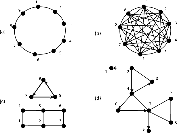
We first evaluate the distributed learning algorithm with different choices of temperature on the interference graph (d) in Figure 5. We run the learning algorithm sufficiently long until the time average system throughput does not change. The result in Figure 7 shows the system performance with different , and demonstrates that a proper temperature can achieve a balance between exploration and exploitation and offer the best performance. When is small, the users tend to select the channels randomly (i.e., over-exploration) and the performance gap can be large. When is very large, the algorithm focuses on exploitation and may get stuck in local optimum and the performance is again negatively affected. In the following simulations we set since it achieves good system performance in both random backoff and Aloha mechanisms as in Figure 7.
We then evaluate the convergence of the distributed learning algorithm. In Figure 7, we show the number of iterations for the convergence of distributed learning algorithm with random backoff and Aloha mechanisms. We see that, as the interference graph becomes more dense (e.g., graph (b)), the convergence time becomes longer. The reason is that, when the interference graph becomes more dense and a user can generate interference to more users, the environment becomes more complex and it hence takes more time overhead to explore. We also observe that the convergence time of Aloha mechanism is longer than that of random backoff mechanism. This is because that in Aloha mechanism users are heterogeneous in terms of channel contention capability and hence the system environment becomes more complicated.


We further compare distributed learning with the solutions obtained by the following algorithms:
- •
Random Access: each user chooses a channel to access purely randomly.
- •
Multi-armed Bandit: we implement the multi-armed bandit solution for distributed spectrum access in [36].
- •
Mixed NE: we compute the exact mixed Nash equilibrium of the spatial spectrum access game, based on statistical network information using the global Newton method [25].
- •
Dynamic Game: we compute the solution of the complete information dynamic game for spectrum access, by solving the corresponding stage spatial spectrum access game (using the global Newton method) for each time slot , with the channel idle probabilities of the stage game replaced by the channel state realization of time slot .
- •
Centralized Optimization: the solution obtained by solving the centralized global optimization of .
We implement these algorithms together with the distributed learning algorithm on the four types of interference graphs in Figure 5. The results are shown in Figures 9 and 9. We see that the exact mixed Nash equilibrium of spatial spectrum access game based on statistical network information is efficient, with a less than performance loss compared with the dynamic game solution. This is because that in the proposed spatial spectrum access game, each secondary user takes both the primary activity levels on different channels and the competition with other secondary users into consideration. This can help to mitigate the congestion within secondary users and exploit the channels of high transmission opportunities. Moreover, the performance gap of the approximate mixed Nash equilibrium by distributed learning from the exact mixed Nash equilibrium is small, with a less than performance loss in all cases. For the random backoff (Aloha, respectively) mechanism, we see that the distributed learning algorithm achieves up-to (, respectively) performance improvement over the random access algorithm. Moreover, we observe that the distributed learning algorithm can achieve better performance than the multi-armed bandit scheme, with a performance gain of up-to . This is because that the design of multi-armed bandit scheme does not take the spatial reuse effect in account. Compared with the centralized optimal solution, the performance loss of the distributed learning in the full-interference graph (b) is (, respectively). Such performance loss is not due to the algorithm design; instead it is due to the selfish nature of the users (i.e., competition in distributed spectrum sharing). In the partial-interference graphs (a), (c), and (d), the performance loss can be further reduced to less than (, respectively). This shows that the negative impact of users’ selfish behavior is smaller when users can share the spectrum more efficiently through spatial reuse.
IX Conclusion
In this paper, we explore the spatial aspect of distributed spectrum sharing, and propose a framework of spatial spectrum access game on directed interference graphs. We investigate the critical issue of the existence of pure Nash equilibria, and develop a distributed learning algorithm converging to an approximate mixed Nash equilibrium for any spatial spectrum access games. Numerical results show that the algorithm is efficient and has significant performance gain over a random access algorithm that does not take the spatial effect into consideration.
For the future work, we are going to design distributed spectrum access mechanisms that can converge to pure Nash equilibria for those spatial spectrum games which are not potential games but admit pure Nash equilibria. We will also study the general spatial spectrum access game under the physical interference model.
References
- [1] X. Chen and J. Huang, “Spatial spectrum access game: Nash equilibria and distributed learning,” in Proceedings of the thirteenth ACM international symposium on Mobile Ad Hoc Networking and Computing (MOBIHOC). ACM, 2012, pp. 205–214.
- [2] I. Akyildiz, W. Lee, M. Vuran, and S. Mohanty, “Next generation/dynamic spectrum access/cognitive radio wireless networks: a survey,” Computer Networks, vol. 50, no. 13, pp. 2127–2159, 2006.
- [3] B. Wang, Y. Wua, and K. R. Liu, “Game theory for cognitive radio networks: An overview,” Computer Networks, vol. 54, pp. 2537–2561, 2010.
- [4] N. Nie and C. Comniciu, “Adaptive channel allocation spectrum etiquette for cognitive radio networks,” in Proc. of IEEE DySPAN, Baltimore, USA, Nov. 2005.
- [5] D. Niyato and E. Hossain, “Competitive spectrum sharing in cognitive radio networks: a dynamic game approach,” IEEE Transactions on Wireless Communications, vol. 7, pp. 2651–2660, 2008.
- [6] M. F¨¦legyh¨¢zi, M. Cagalj, and J.-P. Hubaux, “Efficient mac in cognitive radio systems: A game-theoretic approach,” IEEE Transactions on wireless Communications, vol. 8, pp. 1984–1995, 2009.
- [7] Z. Han, C. Pandana, and K. J. R. Liu, “Distributive opportunistic spectrum access for cognitive radio using correlated equilibrium and no-regret learning,” in Proc. of IEEE WCNC, Hong Kong, March 2007.
- [8] A. Anandkumar, N. Michael, and A. Tang, “Opportunistic spectrum access with multiple users: learning under competition,” in Proc. of IEEE INFOCOM, San Diego, USA, March 2010.
- [9] K. Liu and Q. Zhao, “Decentralized multi-armed bandit with multiple distributed players,” in Proc. of IEEE IAT, San Diego, USA, Jan. 2010.
- [10] M. Weiss, M. Al-Tamaimi, and L. Cui, “Dynamic geospatial spectrum modelling: taxonomy, options and consequences,” in Proc. of TPRC Conference, Fairfax, USA, Sep. 2010.
- [11] C. Tekin, M. Liu, R. Southwell, J. Huang, and S. Ahmad, “Atomic congestion games on graphs and their applications in networking,” EEE/ACM Transactions ON Networking, vol. 20, no. 5, Oct. 2012.
- [12] V. Bilò, A. Fanelli, M. Flammini, and L. Moscardelli, “Graphical congestion games with linear latencies,” in Proc. of ACM SPAA, Munich, Germany, June 2008.
- [13] X. Chen and J. Huang, “Spatial spectrum access game,” The Chinese University of Hong Kong, Tech. Rep., 2013. [Online]. Available: http://www.public.asu.edu/~xchen179/SSAG.pdf
- [14] FCC, “Second memorandum opinion and order,” September 23, 2010. [Online]. Available: http://transition.fcc.gov/Daily_Releases/Daily_Business/2010/db0923/FCC-10-174A1.pdf
- [15] H. Anouar and C. Bonnet, “Optimal constant-window backoff scheme for ieee 802.11 dcf in single-hop wireless networks under finite load conditions,” Wireless Personal Communications, vol. 43, no. 4, pp. 1583–1602, 2007.
- [16] J. Nash, “Equilibrium points in n-person games,” Proceedings of the National Academy of Sciences, vol. 36, pp. 48–49, 1950.
- [17] N. Biggs, E. Lloyd, and R. Wilson, Graph Theory. Oxford University Press, 1986.
- [18] P. Santi, “Topology control in wireless ad hoc and sensor networks,” ACM Computing Surveys (CSUR), vol. 37, no. 2, pp. 164–194, 2005.
- [19] I. Milchtaich, “Congestion games with player-specific payoff functions,” Games and Economic Behavior, vol. 13, pp. 111–124, 1996.
- [20] D. Monderer and L. S. Shapley, “Potential games,” Games and Economic Behavior, vol. 14, pp. 124–143, 1996.
- [21] M. Mavronicolas, I. Milchtaich, B. Monien, and K. Tiemann, “Congestion games with player-specific constants,” Mathematical Foundations of Computer Science 2007, pp. 633–644, 2007.
- [22] J. H. Monisha and V. R. Uthariaraj, “User profile based proportional share scheduling and mac protocol for manets,” International Journal of Distributed and Parallel Systems (IJDPS), vol. 3, no. 1, pp. 269–283, Jan. 2012.
- [23] E. Koutsoupias and C. Papadimitriou, “Worst-case equilibria,” in STACS 99. Springer, 1999, pp. 404–413.
- [24] J. Marden, H. Young, G. Arslan, and J. Shamma, “Payoff-based dynamics for multiplayer weakly acyclic games,” SIAM Journal on Control and Optimization, vol. 48, no. 1, pp. 373–396, 2009.
- [25] S. Govindan and R. Wilson, “A global newton method to compute nash equilibria,” Journal of Economic Theory, vol. 110, pp. 65–86, 2003.
- [26] X. Chen and J. Huang, “Imitative spectrum access,” in Proc. of IEEE WiOpt, Paderborn, Germany, May 2012.
- [27] M. Maskery, V. Krishnamurthy, and Q. Zhao, “Decentralized dynamic spectrum access for cognitive radios: Cooperative design of a non-cooperative game,” IEEE Transactions on Communications, vol. 57, no. 2, pp. 459–469, 2009.
- [28] D. Shah and J. Shin, “Dynamics in congestion games,” ACM SIGMETRICS Performance Evaluation Review, vol. 38, no. 1, pp. 107–118, 2010.
- [29] R. Cominetti, E. Melo, and S. Sorin, “A payoff-based learning procedure and its application to traffic games,” Games and Economic Behavior, vol. 70, no. 1, pp. 71–83, 2010.
- [30] H. Kushner and G. Yin, Stochastic Approximation and Recursive: Algorithms and Applications. New York: Springer-Verlag, 2003.
- [31] C. Daskalakisa, A. Mehtab, and C. Papadimitriou, “A note on approximate Nash equilibria,” Theoretical Computer Science, vol. 410, no. 17, pp. 1581–1588, 2009.
- [32] Y. Shi, Y. T. Hou, J. Liu, and S. Kompella, “How to correctly use the protocol interference model for multi-hop wireless networks,” in Proceedings of the tenth ACM international symposium on Mobile ad hoc networking and computing. ACM, 2009, pp. 239–248.
- [33] X. Zhou, Z. Zhang, G. Wang, X. Yu, B. Y. Zhao, and H. Zheng, “Practical conflict graphs for dynamic spectrum distribution,” in Proceedings of the ACM SIGMETRICS/international conference on Measurement and modeling of computer systems. ACM, 2013, pp. 5–16.
- [34] P. Gupta and P. R. Kumar, “The capacity of wireless networks,” IEEE Transactions on Information Theory, vol. 46, no. 2, pp. 388–404, 2000.
- [35] L. Yang, L. Cao, and H. Zheng, “Physical interference driven dynamic spectrum management,” in 3rd IEEE Symposium on New Frontiers in Dynamic Spectrum Access Networks. IEEE, 2008, pp. 1–12.
- [36] L. Lai, H. El Gamal, H. Jiang, and H. V. Poor, “Cognitive medium access: Exploration, exploitation, and competition,” IEEE Transactions on Mobile Computing, vol. 10, no. 2, pp. 239–253, 2011.
- [37] S. Boyd and L. Vandenberghe, Convex optimization. Cambridge university press, 2004.
X Appendix
X-A Proof of Lemma 1
Suppose that the original spatial spectrum access game on the interference graph has a pure Nash equilibrium We index the newly added player as player , denote the set of players that can generate interference to player as , and denote the set of player ’s interfering players that choose channel as . Now player can compute its best response strategy . Obviously, the strategy profile of players in the new game is a pure Nash equilibrium. ∎
X-B Proof of Lemma 2
Suppose that the original spatial spectrum access game has a pure Nash equilibrium We index the newly added player as player . Now player can compute its best response strategy as follows.
Case : if player does not have an interference relationship with any player in the original game, then
| (28) |
In this case, the strategy profile of players in the new game is a pure Nash equilibrium.
Case : if player can not generate interference to any player in the original game, and there is one player that can generate interference to player , then
| (29) |
According to Lemma 1, the strategy profile must be a pure Nash equilibrium of the new game.
Case : If player can generate interference to a player in the original game, then player can compute its best response strategy according to (29) if player can also generate interference to player , and according to (28) otherwise. By checking that whether and are the same, we have the following two possibilities.
1) If , then the strategy profile must be a pure Nash equilibrium for the new game.
2) If , we modify the original game as follows. For player , we modify the utility function as if and otherwise. For any other player and , we keep the utility function unchanged, i.e., For the modified game with the utility function , it is easy to check that it also satisfies the congestion property and hence it has a pure Nash equilibrium by assumption (since this game is still played over the same given interference graph and any game satisfying the congestion property on original interference graph has a pure Nash equilibrium by assumption). If , the strategy profile is a pure Nash equilibrium for the new game with players, since given the interference between player and player , any player is playing the best response strategy. If , we can show that the strategy profile is still a pure Nash equilibrium for the new game. This is because that, without the interference between player and player (since they play different strategies), playing strategy can not be worse due to the congestion property and hence is still player ’s best response. For any player in the original game, playing is the best response strategy given player ’s strategy . ∎
X-C Proof of Theorem 3
We first consider the complete bipartite graph. Since the interference graph is bipartite, we can decompose the set of vertices into two disjoint sets and . Let denote the number of vertices in set for . Without loss of generality, we will assume that . According to the definition of bipartite graph, we see that two users can generate interference to each other if and only they are from different sets.
Recall that the channel grabbing probability of the random backoff mechanism is given in (3). We define that , where is the number of contending users with user . We then order the channels such that . If , we can trivially construct a pure Nash equilibrium by assigning each user with channel . If we can construct a pure Nash equilibrium by assigning users in set with channel and users in set with channel . In this case, the throughput of a user in set is and the throughput of a user in set is No user has the incentive to deviate.
For the regular bipartite graph case, we define that where is the node degree of the graph (i.e., the number of edges connected by each node). It is then easy to check that the above procedure of constructing pure Nash equilibrium is still valid. ∎
X-D Proof of Theorem 5
For the ease of exposition, we first define that
Thus, we have .
Now suppose that a user unilaterally changes its strategy to , such that the strategy profile changes from to . We have that
| (30) |
For the part , we have
| (31) |
For the part , we have
This implies that
| (32) |
Similarly, we have that
| (33) |
X-E Proof of Theorem 6
We first define that an . It is easy to check that
| (34) |
Since the random backoff mechanism is adopted, according to (3), we have that
| (35) |
By Theorem 4, we know that the spatial spectrum access game with throughput function on any undirected graph is a potential game with potential function . It hence follows from (34) and (35) that the spatial spectrum access game with throughput function in (17) on any undirected graph is also a potential game with potential function . ∎
X-F Proof of Theorem 7
For the ease of exposition, we first define , , and
Thus, we have .
Now suppose that a user unilaterally changes its strategy to . Let be the new strategy profile. Thus, the change in potential from to is given by
| (36) |
Equation (36) consists of three parts. Next we analyze each part separately. For the first part, we have
| (37) |
For the second part in (36),
This means
| (38) |
For the third term in (36), we can similarly get
| (39) |
Substituting (37), (38), and (39) into (36), we obtain
| (40) |
Since and
we can conclude that is a potential function. ∎
X-G Proof of Theorem 8
First of all, since , we know that . Thus, it follows that
| (41) |
Suppose that is an arbitrary Nash equilibrium of the spatial spectrum access game . Then at Nash equilibrium, we must have that
| (42) |
Otherwise, the user can always improve its payoff by choosing the channel that maximizes , which would contradict with the fact that is a Nash equilibrium. According to (41) and (42), we then obtain that
| PoA | ||||
∎
X-H Proof of Lemma 3
This proof is derived based on the one in [29]. The key difference is that we consider that the generalized spatial congestion games on any generic graphs and users can be heterogenous. While, [29] only considers the special case that the congestion game is defined over the complete graphs and users are homogenous.
According to (23), we first compute the expected payoff as
| (43) |
X-I Proof of Theorem 10
We first consider the following optimization problem for each user
| (48) | ||||
| subject to |
Recall that denotes the throughput of user choosing channel given that other users adhere to the perceptions (i.e., other users’ mixed strategies since ). Then the objective function (48) is to choose a mixed strategy for user to maximize its expected throughput off the term . The constraint is to ensure that the mixed strategy is feasible.
X-J Proof of Theorem 11
We first define that . According to (27), we first have that
Since is a a monotonically strictly increasing function, we have that
Suppose a user changes its channel to such that strategy profile changes from to . We have that
Since denotes the distance between user and user , we have . Thus,
It follows that
∎