Author’s address: X. Qiu, Department of Computer Science and Engineering, Ohio State University, Columbus, OH 43210, USA.
Topic words analysis based on LDA model
Abstract
Social network analysis (SNA), which is a research field describing and modeling the social connection of a certain group of people, is popular among network services. Our topic words analysis project is a SNA method to visualize the topic words among emails from Obama.com to accounts registered in Columbus, Ohio. Based on Latent Dirichlet Allocation (LDA) model, a popular topic model of SNA, our project characterizes the preference of senders for target group of receptors. Gibbs sampling is used to estimate topic and word distribution. Our training and testing data are emails from the carbon-free server Datagreening.com. We use parallel computing tool BashReduce for word processing and generate related words under each latent topic to discovers typical information of political news sending specially to local Columbus receptors. Running on two instances using paralleling tool BashReduce, our project contributes almost 30% speedup processing the raw contents, comparing with processing contents on one instance locally. Also, the experimental result shows that the LDA model applied in our project provides precision rate 53.96% higher than TF-IDF model finding target words, on the condition that appropriate size of topic words list is selected.
1 Introduction
Social network is a network consisting of constant information of the connection of a group of people. Social Network Analysis (SNA) [2] discovers the unique or target characters to describe the certain pattern of such people connection. As an implementation of SNA, online social services like LinkedIn.com are becoming popular these years. In some previous studies, SNA models are implemented to make connections of certain groups by directed graph models or weighted edge graph models. For example, Wang and his coworkers develop a probabilistic factor graph model [16] to analyze bibliographic network in academic world. When conducting research in social networks by characterizing documents, such as emails and academic publications, data mining models have been applied in many SNA models. Lada Adamic and Eytan Adar present Latent Dirichlet Allocation (LDA) model [3], which selects Dirichlet distribution to estimate topic mixture, and samples training data by Expectation Maximization (EM) algorithm. This LDA model collects separated data to improve predicted models, generating representative words under such latent topics from given documents. Later, Rosen-Zvi and her group extend LDA model to Author Topic (AT) model [14], determining topics by both content and author distributions.
Our project collects topic words from emails and models the preference of senders in typical website, using Gibbs sampling as training strategy instead of EM algorithm. We create an email account at Columbus, Ohio and use this account to register at Obama.com. Emails sent by Obama.com are received through Datagreening.com [15], which is a carbon-free server developed by our research group. Then the downloaded emails are processed to input data for LDA model in an appropriate format. Then we apply the LDA model mapping the data to topic layers. Thus the topic words list is able to be generated in the next step. Finally, by analyzing the similarity between target words list and topic words list generated in above steps, we establish which information are likely given to publicity by Obama.com.
Python packages have been used to process words, such as word tokenizing, word stemming and filtering out stop words, etc. Word count program is run on two nodes implementing the parallel computing tool BashReduce [17] to achieve almost 30% speedup. TF-IDF model [11] is selected to be a comparison generating topic words list. The model applied in our project provides precision rate 53.96% higher than TF-IDF model, when we define the size of topic list properly.
The rest parts of this paper are organized in following five sections: In section 2, we introduce the generative LDA model and the design details of applying this model in our project. Section 3 describes parameter estimation using Gibbs sampling [10]. Section 4 describes Datagreening.com server, BashReduce tool and python packages used in the project. Experimental results are shown and evaluated in section 5. Conclusion and future work are discussed in section 6.
2 Generative LDA Model
In this section, we will first briefly introduce the unigram model, a model generating documents by single topics. Then we discuss LDA model applied in our project. To simplify the process, we define that a document is a collection of discrete words.
2.1 Unigram Model
Unigram Model, which is a basic probability model, treats words as isolated elements in each document [13]. Assume that we have a corpus of documents, and a document d is a vector of words, where each word is selected from a vocabulary of words. We define document , and corpus . In unigram model, the probability of generating document is:
| (1) |
Considering that the documents are interchangeable with each other, the probability of generating corpus is:
| (2) |
Suppose the word probability of this corpus is , and the probability of word in corpus is . Then written in full, can be representative as a multinomial distribution over words vocabulary:
| (3) |
where is the vector of words probability in vocabulary, and the probability of the corpus is .
2.2 LDA Model
LDA model is a Bayesian hierarchy topic model [8], generating topic words for each document with efficiently reduced complexity. Also, LDA model characterize the possibility that one document may contain multiple topics, while unigram model only consider the single topic situation. Instead of calculating probability of word frequency using continually multiply in unigram model, LDA model maps a document of words to latent topics. As the hierarchy model shows in Figure 1, document-word distribution has been mapped to document-topic distribution following topic-word distribution. Therefore, the general expression for word probability in topic model is:
| (4) |
where is the th topic sampled from a multinomial distribution of which the prior distribution is a Dirichlet distribution.

In our project, a document of words is generated in the following process. Suppose that there are latent topics, then the probability of th word in the given document can be represented in the following mixture:
| (5) |
where is the topic to which th word assigned, represents the probability of word assigned to the th topic, and gives the topic mixture proportion for the current sampled document. Assume that the corpus is a collection of documents and the vocabulary of this corpus has unique words. Each document of words is generated according to topics. Let denote , representing that word is sampled from the multinomial distribution on the th topic . And let denote , which is a multinomial distribution from topics for document . Therefore, the probability of word in document is:
| (6) |
In LDA model, sampled from is the prior distribution of multinomial distribution [9], and sampled from symmetric is the prior distribution of multinomial distribution . Then the multinomial distributions and in LDA model is parameterized as follows:
| (7) |
| (8) |
In Eq.(7), is a matrix, which is the initial value of word probability sampled from topics. And in Eq.(8), is the initial value of topic probability. and are parameters of prior distribution of each multinomial distribution. We assume both prior distributions to be symmetric Dirichlet distributions. Therefore, is initialed the same value in the beginning of sampling every document. Also, is initialed the same value in the beginning of sampling every document.
Figure 2 shows the Bayesian network [4] of LDA model. The plates represent repeated sampling. In the left part, the inner plate represents generating each topic and each word under its topic repeatedly in a document ; the outer plate represents repeated sampling topic proportion for each of documents in corpus. And the right plate repeatedly samples parameters for .

3 Gibbs Sampling
To estimate parameters of LDA model, Lada Adamic and Eytan Adar use Expectation Maximization (EM) algorithm as the inference strategy [12]. In our project, Gibbs sampling is the choice. Considering the posterior distribution , Gibbs sampling is a simple strategy to estimate and . As a simple case of Markov chain Monte Carlo (MCMC) algorithm, Gibbs sampling aims at constructing a Markov chain converging to the target distribution on , and selecting samples approximating the inferred distribution. The sampling method begins with initialing the value of vector . Then it repeatedly samples the from the conditional probability and transfers to the next state of Markov chain by updating the probability function using the newly sampled . In our project, the probability function of Gibbs sampling is:
| (9) |
where stands for the assignment of word , the th word in a document, to topic ; and represents all assignments. is the number of times assigned to topic ; is the number of words in vocabulary assigned to topic ; is the number of words in document assigned to topic ; all numbers of words do not include the current assignment .
The detailed sampling process is as follows:
- 1.
For to , where is the number of word in the current document, iteratively initial as one random integer between to . This -sized vector is the initial state of this Markov chain.
- 2.
For to , transfer to next state of this Markov chain by iteratively assigning word to its topic using Eq.(9).
- 3.
Run step 2 for iterations until it reaches the convergent state. For to , the current value of is selected as a sample. The value of is called Burn-in period in Gibbs sampling.
Eq.(9) is the function calculating the posterior distribution over word distribution in each document. Therefore, we can derive the conditional probability function estimating and for every unique word in a document by removing the word tag in Eq.(9):
| (10) |
where is the number of times assigned to topic ; is the number of words in vocabulary assigned to topic ; is the number of words in document assigned to topic ; is the number of all words in document assigned to its topic.
4 Data Preprocessing
In this section, we discuss the operations of data preprocessing for LDA model. Datagreening.com server, Python packages and BashReduce tool implemented in our project will be introduced in the following.
4.1 Datagreening.com
The input data for analyzing in LDA model are emails sent to our locally registered account at Obama.com. In our project, these emails are received through Datagreening.com, which is an email server developed by our research group. This server provides email service with clean energy and collects research data of carbon footprint in the meantime. Also, capturing the energy cost in datacenters of popular email providers, this greening server helps further research in performance of cloud computing.
4.2 Python packages
The downloaded emails are processed to documents consisting of unique terms using Python NumPy package [7] and Natural Language Toolkit (NLTK) package [5]. NumPy is the fundamental package for scientific computing with Python. We install the NumPy package to offer the proper back environment for NLTK packages and include sorting algorithm functions for Python code. NLTK is a Python platform for text processing. Some of the NLTK packages are installed for raw content tokenizing, word stemming and stop words removing in our project. Following is the list of packages we installed:
- 1.
banktree_tag package;
- 2.
stop_word package;
- 3.
wn package.
4.3 BashReduce tool
Now we format the unique terms learned by the above Python program as:
where N is the number of unique terms in the current document; word_i is an integer that indexes this term in the vocabulary. BashReduce tool is used here to calculate the word count.
BashReduce is a parallel computing tool applying online MapReduce [6] model to bash environment. According to BashReduce operation instruction, we begin with specifying the host list to be bash.xi.0 and bash.xi.1 using BashReduce option ’br –h’. Thus, we have two instances for parallel calculating word count. Then we write Python programs map.py and reduce.py. Program map.py maps each word in word set to pattern (word,1); while reduce.py receives such patterns and sum the same patterns to generate the (word, count) result and implements. We use BashReduce options ’-m’ and ’-r’ to run map.py and reduce.py respectively. Note that, both input and output paths for map.py and reduce.py need to be defined by user. Running on two instances implemented BashReduce, it costs 3’41” to finish the word count program, ignoring the network latency. Comparing with the time cost 5’18” when calculating locally, it achieve almost 30% speedup.
5 Experimental Result
In our results, we use emails sent to our locally registered account by Obama.com. There are total 58 emails in this account with a vocabulary size of words. To use Gibbs sampling more efficiently, we first fix the value of burn-in period using the data learned in section 4. Then we show the experimental result of top 15 words generated under 5 latent topics. And we define precision rate to evaluate the predictive power.

5.1 Burn-in period choice
We define the number of topics and use 3 distinct values for initialization. Then the convergent sample result will be obtained when choosing the appropriate iteration number.
Figure 3 shows the convergent process for Gibbs sampling. Starting at 3 distinct values, the sample result tends to gather and reach a constant value independent with all three initial values after 500 iterations.
5.2 Experimental Result
In our experiment, parameters and are assigned values 0.01 and respectively. Latent topics are selected after 500 iterations in Gibbs sampling. And words are generated under 300 topics. Table 1 give the example of top 15 words generated under 4 topics.
Example of top 15 words generated under 5 topics. Topic1 Topic2 Topic3 Topic4 Topic5 action winner ohio display president organize enter party color obama email guest help none contact make action need medium supporter take organize governor screen committee get nbsp state input email ofa washington authorize block democrat people receive friend auto let health contribution make http washington fight entry kasich label work send email campaign leave know care state pay nbsp candidate Box ticke republican see support friend prize voter table country address resident Work Arial stay {tabnote} \tabnoteentryaWords in each topic list is able to help reveal what corresponding topic it can be. According to the table, a email from Obama.com is likely consisting of health care (Topic1), new contributions (Topic2), local news (Topic3), and president information (Topic4).
5.3 Result Analysis
To compare the LDA model applied in our project with other models, we intuitively define a word list of size , and each word in the target list works as an identifier to represent the information of this corpus.
correct list = {obama, ohio, health, washington, governor,campaign, republican, president, party, supporter, state, committee,democrat, voter, work}
And the target word list are defined as part of the correct list.
5.3.1 Evaluation measure
We use precision as a measure to evaluate the experimental results. The definition of precision is defined as follow:
| (11) |
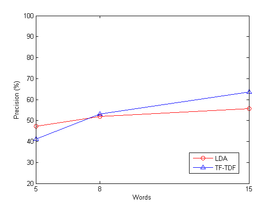
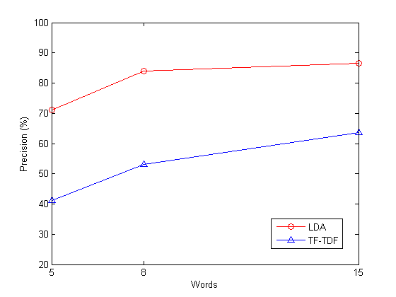
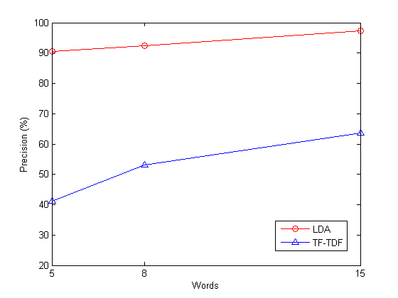
For each document with topic word list, we compare the top words of each topic words list with the words in current target word list. If any match is captured, then we mark this document as ’correct’. in Eq.(11) represents the number of ’correct’ documents in this corpus, and stands for the total number of documents in this corpus.
5.3.2 Comparison model
We choose TF-IDF model as a comparison.TF-IDF, short for Term Frequency-Inverse Document Frequency model, a numerical statistic representing the relation between the key word and the document, is one of the major weight factors in text mining. It is often used for text classification by ranking a document’s relevance given a user query. Assume that is the total number of dicuments in this corpus; is the raw frequency of a term in a document, then the expression of this model is:
| (12) |
where is defined as:
| (13) |
Therefore, a high weight in TF-IDF is reached by a high term frequency and a low document frequency of the term in the whole collection of documents; the weights hence tend to filter out common terms and select the terms with lower probability to be the words that distinguish documents.
5.3.3 Predictive power
Let be denoted as the size of target word list, and as the size of topic word list. We evaluate the predictive power by comparing precision rate for LDA model and TF-IDF model in cases with different —. The following Figure 4, Figure 5 and Figure 6 show the comparison of LDA model and TF-IDF model where x-coordinate represents different values of and y-coordinate represents precision rate.
6 Conclusion
In this project, we apply LDA model to analyze and vilsualize topic words of emails from Obama.com to accounts registered in Columbus, Ohio. We use Gibbs sampling to estimate topic and word distribution. Carbon-free server Datagreening.com, pareleling tool BashReduce and Python packages are used in data preprocessing. The experimental result shows the MapReduce method in our project efficiently reduces the time cost of word count program and the predictive power of LDA model applied in our project is obviously stronger than TF-IDF model.
Every new document adding to this corpus lead to another sampling process for it, highly increasing the time cost. Considering this drawbask, possible future work of our project is likely to be sampling only new added words instead of a new added document.
References
- Adamic and Adar (2009) Lada A. Adamic and Eytan Adar. 2009. How to search a social network. @MISC. (2009). http://arXiv.org/abs/cond-mat/0310120
- Blei et al. (2003) David M. Blei, Andrew Y. Ng, and Michael I. Jordan. 2003. Latent Dirichlet Allocation. J. Mach. Learn. Res. 3 (March 2003), 993–1022. http://dl.acm.org/citation.cfm?id=944919.944937
- Carey (2003) Vincent J Carey. 2003. Graphical models: Methods for data analysis and mining. J. Amer. Statist. Assoc. 98, 461 (2003), 253–254.
- Dan Garrette and Nothman (2013) Peter Ljunglöf Dan Garrette and Joel Nothman. 2013. Python text processing package NLTK. (2013). http://www.nltk.org/api/nltk.html
- Dean and Ghemawat (2008) Jeffrey Dean and Sanjay Ghemawat. 2008. MapReduce: simplified data processing on large clusters. Commun. ACM 51, 1 (2008), 107–113.
- Developers (2013) NumPy Developers. 2013. Python scientific computing package NumPy. (2013). http://www.numpy.org
- Fei-Fei and Perona (2005) L. Fei-Fei and P. Perona. 2005. A Bayesian hierarchical model for learning natural scene categories. In Computer Vision and Pattern Recognition, 2005. CVPR 2005. IEEE Computer Society Conference on, Vol. 2. 524–531. DOI:http://dx.doi.org/10.1109/CVPR.2005.16
- Forbes et al. (2011) Catherine Forbes, Merran Evans, Nicholas Hastings, and Brian Peacock. 2011. Statistical distributions. John Wiley & Sons.
- Gilks et al. (1996) WR Gilks, S Richardson, DJ Spiegelhalter, and others. 1996. Markov Chain Monte Carlo in Practice. 1996. New York: Chapman Hall/CRC 486 (1996).
- Liu et al. (2004) Ying Liu, B.J. Ciliax, K. Borges, V. Dasigi, A. Ram, S.B. Navathe, and R. Dingledine. 2004. Comparison of two schemes for automatic keyword extraction from MEDLINE for functional gene clustering. In Computational Systems Bioinformatics Conference, 2004. CSB 2004. Proceedings. 2004 IEEE. 394–404. DOI:http://dx.doi.org/10.1109/CSB.2004.1332452
- McCallum (1999) Andrew McCallum. 1999. Multi-label text classification with a mixture model trained by EM. In AAAI’99 Workshop on Text Learning. 1–7.
- Nigam et al. (2000) Kamal Nigam, AndrewKachites Mccallum, Sebastian Thrun, and Tom Mitchell. 2000. Text Classification from Labeled and Unlabeled Documents using EM. Machine Learning 39, 2-3 (2000), 103–134. DOI:http://dx.doi.org/10.1023/A:1007692713085
- Rosen-Zvi et al. (2004) Michal Rosen-Zvi, Thomas Griffiths, Mark Steyvers, and Padhraic Smyth. 2004. The Author-topic Model for Authors and Documents. In Proceedings of the 20th Conference on Uncertainty in Artificial Intelligence (UAI ’04). AUAI Press, Arlington, Virginia, United States, 487–494.
- Stewart (2012) Christopher Stewart. 2012. A prototype greening service that powers email with clean energy. @MISC. (2012). http://www.datagreening.com
- Wang et al. (2010) Chi Wang, Jiawei Han, Yuntao Jia, Jie Tang, Duo Zhang, Yintao Yu, and Jingyi Guo. 2010. Mining Advisor-advisee Relationships from Research Publication Networks. In Proceedings of the 16th ACM SIGKDD International Conference on Knowledge Discovery and Data Mining (KDD ’10). ACM, New York, NY, USA, 203–212. DOI:http://dx.doi.org/10.1145/1835804.1835833
- Zawodny (2009) Jeremy Zawodny. 2009. A Bare-Bones MapReduce. @MISC. (2009). http://www.linux-mag.com/id/7407/