UMISS-HEP-2014-01 The Azimuthal Angular Distribution with Tensor Operators
Abstract
In a recent paper we performed a comprehensive study of the impact of new-physics operators with different Lorentz structures on decays, , involving the transition. In this work we extend the previous calculation by including tensor operators. In the case of , we present the full three angle and angular distribution with tensor new physics operators with complex couplings. The impact of the tensor operators on various observables in the angular distribution, specially the azimuthal observables including the CP violating triple product asymmetries are discussed. It is shown that these azimuthal observables are very useful in discriminating different new physics operators. Finally we consider new physics leptoquark models with tensor interactions and show how the presence of additional scalar operators modify the predictions of the tensor operators.
1 Introduction
The search for new physics(NP) beyond the Standard Model (SM) of particle physics is going on at the energy frontier in colliders such as the LHC and at the intensity frontier at high luminosity experiments. In the intensity frontier, the B factories, BaBar and Belle, have produced an enormous quantity of data and there is still a lot of data to be analyzed from both experiments. The LHCb and Belle II will continue the search for NP through precision measurements in the b quark system. There are a variety of ways in which NP in B decays can be observed [1]. In this NP search, the second and third generation quarks and leptons may be quite special because they are comparatively heavier and could be relatively more sensitive to NP. As an example, in certain versions of the two Higgs doublet models (2HDM) the couplings of the new Higgs bosons are proportional to the masses and so NP effects are more pronounced for the heavier generations. Moreover, the constraints on NP involving, specially the third generation leptons and quarks, are somewhat weaker allowing for larger NP effects [2].
The semileptonic decays of B meson to the lepton is mediated by a boson in the SM and it is quite well understood theoretically. In many models of NP this decay gets contributions from additional states like new vector bosons, leptoquarks or new scalar particles. These new states can affect the semileptonic and transitions. The exclusive decays and are important places to look for NP because, being three body decays, they offer a host of observables in the angular distributions of the final state particles. The theoretical uncertainties of the SM predictions have gone down significantly in recent years because of the developments in heavy-quark effective theory (HQET). The experimental situation has also improved a lot since the first observation of the decay in 2007 by the Belle Collaboration [3]. After 2007 many improved measurements have been reported by both the BaBar and Belle collaborations and the evidence for the decay has also been found [4, 5, 6]. Recently, the BaBar collaboration with their full data sample of an integrated luminosity 426 fb-1 has reported the measurements of the quantities [7, 8]
| (1) |
where denotes the light lepton . The SM predictions for and are [7, 9, 10]
| (2) |
which deviate from the BaBar measurements by 2 and 2.7 respectively. The BaBar collaboration themselves reported a 3.4 deviation from SM when the two measurements of Eq. (1) are taken together. In this work we do not include the Belle measurements in our average.
These deviations could be sign of NP and already certain models of NP have been considered to explain the data [9, 11, 12, 13, 14, 15, 16, 17, 18, 19, 20, 21, 22, 23, 24, 25]. In Ref. [13], we calculated various observables in and decays with NP using an effective Lagrangian approach. The Lagrangian contains two quarks and two leptons scalar, pseudoscalar, vector, axial vector and tensor operators. Considering subsets of the NP operators at a time, the coefficient of these operators can be fixed from the BaBar measurements and then one can study the effect of these operators on the various observables. In [23] we extended the work of Ref. [13] by providing the full angular distribution with NP. In particular we focused on the CP violating observables which are the triple product (TP) asymmetries [26]. In the SM these TP’s vanish to a very good approximation as the decay is dominated by a single amplitude. Hence, non-zero measurements of these terms are clear signs of NP without any hadronic uncertainties. Note, in the presence of NP with complex couplings the TP’s are non-zero and depend on the form factors. Another probe of CP violation using the decay of the from to multipion decays was recently considered [27].
In this work we include tensor operators in the NP effective Hamiltonian and study their effects on various observables, particularly focusing on the azimuthal observables, including the triple products. Tensor operators were discussed earlier for these decays in [18, 21, 24, 25]. In this work, for , we present the full three angle and angular distribution including tensor new physics operators with complex couplings. This represents the full angular distribution with the most general new physics. In our calculations we focus on the effects of the tensor operators on observables that are sensitive to the azimuthal angle which is the angle between the decay plane of the meson and the off-shell . The triple products are the term proportional to the in the angular distribution. For completeness we will also discuss other observables such as the differential distribution as well as the polarization and forward-backward asymmetries.
Finally, we note that tensor operators are often accompanied by other operators in specific NP models. Hence as an example of tensor operators we consider a leptoquark model that has both tensor and scalar operators. We study how the presence of the scalar operators modify the predictions of the different observables in the angular distribution.
The paper is organized in the following manner. In Sec. 2 we set up our formalism where we introduce the effective Lagrangian for NP with tensor operators and define the various observables in decays. In Sec. 3 we present an explicit leptoquark NP model where we show how tensor operators may arise and consider a few cases. In Sec. 4 we present the numerical predictions which include constraints on the NP couplings as well as predictions for the various observables with NP in . Finally in Sec. 5 summarize the results of our analysis.
2 Formalism
In the presence of NP, the effective Hamiltonian for the quark-level transition can be written in the form [28]
| (3) | |||||
where is the Fermi coupling constant, is the Cabibbo-Kobayashi-Maskawa (CKM) matrix element, are the projectors of negative/positive chiralities. We use and assume the neutrino to be always left chiral. Further, we do not assume any relation between and transitions and hence do not include constraints from . The SM effective Hamiltonian corresponds to .
2.1 angular distribution
The complete three-angle distribution for the decay in the presence of NP can be expressed in terms of four kinematic variables , two polar angles , , and the azimuthal angle . The angle is the polar angle between the charged lepton and the direction opposite to the meson in the rest frame. The angle is the polar angle between the D meson and the direction of the meson in the rest frame. The angle is the azimuthal angle between the two decay planes spanned by the 3-momenta of the and systems. These angles are described in Fig. 1. The three-angle distribution can be obtained by using the helicity formalism:
We can write the angular distribution explicitly for easy comparison with previous literature [29, 30, 31, 32] in terms of the helicity amplitudes
where we can define the and as,
| (5) |
The various helicity amplitudes are defined in the appendix.

It will be convenient to rewrite the angular distribution as [33]
| (6) |
where the quantity is
| (7) |
The momentum of the meson in the B meson rest frame is denoted as with .
The twelve angular coefficients () depend on the couplings, kinematic variables and form factors, and are given in terms of helicity amplitudes in appendix. We use HQET to expand the form factors in terms of certain parameters, which are then fixed from the angular distribution for , where [29]. Our basis assumption is that decays are described by the SM.
The following single-differential angular distributions allow access to various observables that can be used to probe for NP. The differential decay rate can be obtained after performing integration over all the angles
| (8) |
Here the meson’s longitudinal and transverse polarization amplitudes and are
| (9) |
Furthermore, one can also explore the dependent of ratio
| (10) |
By integrating out the polar angles , , and the azimuthal angle in different kinematic regions, various 2-fold angular distributions can be obtained. For a detailed discussions see our previous work [23]. Here, we have updated these angular distributions with the new tensor couplings. Our results agree with the corresponding angular distributions in [25]. Several observables can be defined through the 2-fold angular distributions. The polarization fraction , the forward-backward asymmetry for the leptons, the azimuthal asymmetries, including the three transverse asymmetries , and the three T-odd CP asymmetries , are defined in terms of angular coefficients [23]:
| (11) |
.
In closing this section we note that even though we are focused on the decay the decay is used to constrain the NP operators. The angular distribution, with tensor operators, can be written as,
| (12) | |||||
where the prefactor . The helicity amplitudes are
| (13) |
where and . In addition, the and the amplitudes arise in the combination,
| (14) |
The results in eq.(12) agree with the angular distribution in [25].
3 An Explicit Model
Many extensions of the SM, motivated by a unified description of quarks and leptons, predict the existence of new scalar and vector bosons, called leptoquarks, which decay into a quark and a lepton. These particles carry nonzero baryon and lepton numbers, color and fractional electric charges. The most general dimension four invariant Lagrangian of leptoquarks satisfying baryon and lepton number conservation was considered in Ref [34]. As the tensor operators in the effective Lagrangian get contributions only from scalar leptoquarks, we will focus only on scalar leptoquarks and consider the case where the leptoquark is a weak doublet or a weak singlet. The weak doublet leptoquark, has the quantum numbers under while the singlet leptoquark has the quantum numbers .
The interaction Lagrangian that induces contributions to the process is [18]
| (15) |
where and are the left-handed quark and lepton doublets respectively, while , and are the right-handed up, down quark and charged lepton singlets. Indices and denote the generations of quarks and leptons, and is a charge-conjugated fermion field. The fermion fields are given in the gauge eigenstate basis and one should make the transformation to the mass basis. Assuming the quark mixing matrices to be hierarchical, and considering only the leading contribution we can ignore the effect of mixing. After performing the Fierz transformations, one finds the general Wilson coefficients at the leptoquark mass scale contributing to the process:
| (16) |
It is clear from Eq. (16) that the weak singlet leptoquark and the weak doublet can add constructively or destructively to the Wilson’s coefficients of the scalar and tensor operators in the effective Hamiltonian. We can now consider various scenarios. In the first case the singlet and the doublet scalar leptoquark couplings are such that the scalar operator couplings are enhanced and the tensor operator couplings are suppressed. This scenarios has been studied before [13, 23]. Hence, the first case, called Case. (a), we will study is when the tensor operators is enhanced and the scalar operator suppressed. The results of the pure tensor coupling are presented in the next section.
In this section we will also consider the possibilities where both the scalar and the tensor operators are present and are of similar sizes. In the most general case both the singlet and doublet leptoquarks are present and so both the scalar and tensor operators appear in the effective Hamiltonian. As there is limited experimental information, including both the singlet and the doublet leptoquarks will allow us more flexibility in fitting for the Wilson’s coefficients but this will come with the price of less precise predictions for the various observables. We can, therefore, consider the simpler cases when only a singlet or a doublet leptoquark are present. In these cases, from Eq. (16) the coefficients of scalar operators and the tensor operators have the same magnitudes. One can now consider two further cases:
Case. (b): In this case only the weak doublet scalar leptoquark is present. It was shown recently [35] that this is one of the two minimal renormalizable scalar leptoquark model, where the standard model is augmented only by one additional scalar representation of and which do not allow proton decay at the tree level.
The relations between the scalar and tensor couplings in Eq.16 are valid at the leptoquark mass scale, . We have to run them down to the quark mass scale using the scale dependence of the scalar and tensor currents at leading logarithm approximation
| (17) |
where the anomalous dimensions of the scalar and tensor operators are , respectively and [24]. Choosing a value for the leptoquark mass we can run the couplings to the -quark scale which is chosen to be GeV.
In the simplified scenario with the presence of only one type of leptoquark, namely or , the scalar and tensor Wilson coefficients are no longer independent: one finds that at the scale of leptoquark mass, , . Then, using Eq. (17), one obtains the relation at the bottom mass scale,
| (18) |
for a leptoquark mass of 1 TeV [18].
It is interesting to note that the same coupling that appears in the process also appears in the decay and if the components of the doublet leptoquark have the same mass, then we can have a prediction for this decay based on data from transition.
Case. (c): In this case only the singlet leptoquark is present and the relevant Wilson’s coefficients can be obtained from Eq.16.
4 Numerical analysis
The model independent and dependent numerical results for the various observables in the angular distribution of decay are discussed in this section.
4.1 Model independent results
For the numerical calculation, we use the and form factors in the heavy quark effective theory(HQET) framework [36, 37]. A detailed discussions on the and form factors and their numerical values can be found in [25]. The constraints on the complex NP couplings in the effective Hamiltonian come from the measured and in Eq. (1) at 95% C.L. We vary the free parameters in the HQET form factors within their error bars. All the other numerical values are taken from [38] and [39]. The allowed ranges for the NP couplings are then used for predicting the possible allowed ranges for the observables.
It is important to point out that the combination of couplings appears in both and , while appears only in . and receive constraints from both and . While, the combination of couplings appears only in , appears only in . If NP is established in both and then the cases of pure or or coupling are ruled out. A detailed discussions on the effects of vector and scalar couplings on the various observables in the decays and can be found in our previous works [13, 23].
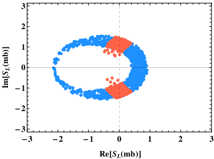
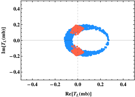
We first consider the Case. (a) of the previous section where only the NP tensor operator is present in the effective Hamiltonian. In Fig. (2), the constraint on the parameter space of the pure tensor coupling by both and measurements at 95% C.L. is shown. We find that the magnitude of tensor coupling satisfies .

The predictions for the differential branching ratio (DBR), , and are shown in Fig. 3 for the allowed values of tensor coupling. It is clear that, the DBR, , and get considerable deviation from their SM expectation in this new physics scenario. The contribution of pure tensor coupling to the forward-backward asymmetry is of the order of , and behaves similar to its SM expectation.


We now wish to analyze the sensitivity of the -integrated azimuthal symmetries on the new tensor coupling, and we present correlations of these symmetries with respect to the integrated forward-backward asymmetry (FBA). The -integrated FBA , the three transverse asymmetries , and the three T-odd CP asymmetries can be obtained by separately integrating out the -dependence in the numerator and denominator of these quantities as expressed in Eq.(11). The panels of Fig.(4) show the correlation between the above six -integrated asymmetries and for the decay . Note that, in this plot we also include predictions for the vector and scalar NP couplings. In each cases, the NP couplings satisfy the current measurements of and at 95% C.L. It is clear from these plots that , and get considerable deviations from their SM expectation once we include the NP couplings. The T-odd CP asymmetry is sensitive to all NP couplings, and is strongly correlated with . The scalar NP couplings can enhance this asymmetry about 5% from its SM value. On the other hand, and are only sensitive to the vector couplings. These asymmetries are also strongly correlated with in the presence of vector NP couplings, and can be enhanced up to 3% from its SM value. Hence, the predictions for and azimuthal symmetries have varying sensitivities to the different NP scenarios and these observables can be powerful probes of the structure of NP.


4.2 Leptoquark model results
We next move to Case.(b) and Case.(c) for the leptoquark with the mass scale of the order of 1 TeV. The allowed ranges for the leptoquark couplings at from the measured and values within the level are shown in Fig. (5). These results suggest that the magnitudes of the doublet and singlet leptoquark effective couplings, and are of . A similar conclusion is obtained in [25].
The correlations between the asymmetries and and are shown in Fig. (6) for three different NP scenarios: only , only leptoquark (), and only leptoquark (). These results imply that and can get sizeable contributions from the leptoquarks within the measured region of . It is interesting to note that the behavior of is different for and leptoquark couplings. Hence this observable can be used to discriminate between the singlet and the doublet leptoquark models.


In Fig.(7) we plot the correlations of and with in the presence of and leptoquark contributions. In each case, the constraints on the leptoquark couplings at are from the current measurements of and within the 2 level. As in the case of pure tensor couplings, these plots show that the different leptoquark models produce very different predictions for the azimuthal asymmetries and so these observables can be very sensitive in ruling out different leptoquark models.


5 Discussion and Summary
In summary we have discussed the effects of tensor operators in the decay motivated by recent measurements which show deviation from the SM predictions in and . In this work we have presented the angular distribution for with the most general new physics structure including tensor operators. We have then discussed the effects of the tensor operators on various observables that can be constructed out of the angular distribution. Our focus was on the azimuthal observables which include the important CP violating triple product asymmetries. We found that these azimuthal asymmetries, integrated over , have different sensitivities to different NP structures and hence they can be powerful probes of the nature of the NP. These asymmetries also show strong correlations with the integrated forward-backward asymmetry. Tensor operators naturally arise in scalar leptoquark models and are accompanied by other scalar operators. We considered two leptoquark models where the leptoquarks are weak singlets and doublets. We discussed the predictions for the azimuthal observables in these models and found that these observables are very efficient in discriminating between the two leptoquark models. In particular we found that there is cancellation between the scalar and tensor components in the scalar doublet leptoquark model for one of the triple product asymmetries while this is not the case for the scalar singlet leptoquark model.
Acknowledgements
This work was supported in part by the National Science Foundation under Grant No. NSF PHY-1068052.
Appendix A Angular coefficients
The twelve angular coefficients in the angular distribution depend on the couplings, kinematic variables and form factors. The expressions for these coefficients are given in terms of the hadronic helicity amplitudes of the decay and summarized according to the helicity combinations :
The longitudinal ’s () are given by
| (19) |
The transverse ’s () are given by
| (20) |
The mixed ’s () are given by
| (21) |
The expressions for the hadronic helicity amplitudes can be found in terms of form factors for the matrix elements [40]
The and the amplitudes arise in the combination
| (23) |
Further, we define the transversity amplitudes and in terms of the helicity amplitudes as
References
- [1] See for e.g. A. Datta, M. Duraisamy and D. Ghosh, Phys. Rev. D 89, 071501 (2014) [arXiv:1310.1937 [hep-ph]]; A. Datta and P. J. O’Donnell, Phys. Rev. D 72, 113002 (2005) [hep-ph/0508314]; A. Datta, Phys. Rev. D 74, 014022 (2006) [hep-ph/0605039]; C. -W. Chiang, A. Datta, M. Duraisamy, D. London, M. Nagashima and A. Szynkman, JHEP 1004, 031 (2010) [arXiv:0910.2929 [hep-ph]]; A. Datta and D. London, Phys. Lett. B 595, 453 (2004) [hep-ph/0404130]; S. Baek, A. Datta, P. Hamel, O. F. Hernandez and D. London, Phys. Rev. D 72, 094008 (2005) [hep-ph/0508149]; A. Datta, M. Imbeault, D. London, V. Page, N. Sinha and R. Sinha, Phys. Rev. D 71, 096002 (2005) [hep-ph/0406192].
- [2] See for example, A. Rashed, P. Sharma and A. Datta, Nucl. Phys. B 877, 662 (2013) [arXiv:1303.4332 [hep-ph]]; A. Rashed, M. Duraisamy and A. Datta, arXiv:1204.2023 [hep-ph]; M. Duraisamy, A. Rashed and A. Datta, Phys. Rev. D 84, 054018 (2011) [arXiv:1106.5982 [hep-ph]]; A. Datta and M. Duraisamy, Phys. Rev. D 81, 074008 (2010) [arXiv:0912.4785 [hep-ph]]; A. Datta, P. J. O’Donnell, Z. H. Lin, X. Zhang and T. Huang, Phys. Lett. B 483, 203 (2000) [hep-ph/0001059].
- [3] A. Matyja et al. [Belle Collaboration], Phys. Rev. Lett. 99, 191807 (2007) [arXiv:0706.4429 [hep-ex]].
- [4] B. Aubert et al. [BABAR Collaboration], Phys. Rev. Lett. 100, 021801 (2008) [arXiv:0709.1698 [hep-ex]].
- [5] I. Adachi et al. [Belle Collaboration], arXiv:0910.4301 [hep-ex].
- [6] A. Bozek et al. [Belle Collaboration], Phys. Rev. D 82, 072005 (2010) [arXiv:1005.2302 [hep-ex]].
- [7] J. P. Lees et al. [BaBar Collaboration], Phys. Rev. Lett. 109, 101802 (2012) [arXiv:1205.5442 [hep-ex]].
- [8] J. P. Lees et al. [BaBar Collaboration], Phys. Rev. D 88, 072012 (2013) [arXiv:1303.0571 [hep-ex]].
- [9] S. Fajfer, J. F. Kamenik and I. Nisandzic, arXiv:1203.2654 [hep-ph].
- [10] Y. Sakaki and H. Tanaka, arXiv:1205.4908 [hep-ph].
- [11] S. Fajfer, J. F. Kamenik, I. Nisandzic and J. Zupan, Phys. Rev. Lett. 109, 161801 (2012) [arXiv:1206.1872 [hep-ph]].
- [12] A. Crivellin, C. Greub and A. Kokulu, Phys. Rev. D 86, 054014 (2012) [arXiv:1206.2634 [hep-ph]].
- [13] A. Datta, M. Duraisamy and D. Ghosh, Phys. Rev. D 86, 034027 (2012) [arXiv:1206.3760 [hep-ph]].
- [14] D. Becirevic, N. Kosnik and A. Tayduganov, Phys. Lett. B 716, 208 (2012) [arXiv:1206.4977 [hep-ph]].
- [15] N. G. Deshpande and A. Menon, arXiv:1208.4134 [hep-ph].
- [16] A. Celis, M. Jung, X. -Q. Li and A. Pich, JHEP 1301, 054 (2013) [arXiv:1210.8443 [hep-ph]].
- [17] D. Choudhury, D. K. Ghosh and A. Kundu, Phys. Rev. D 86, 114037 (2012) [arXiv:1210.5076 [hep-ph]].
- [18] M. Tanaka and R. Watanabe, arXiv:1212.1878 [hep-ph].
- [19] P. Ko, Y. Omura and C. Yu, arXiv:1212.4607 [hep-ph].
- [20] Y. -Y. Fan, W. -F. Wang and Z. -J. Xiao, arXiv:1301.6246 [hep-ph].
- [21] P. Biancofiore, P. Colangelo and F. De Fazio, arXiv:1302.1042 [hep-ph].
- [22] A. Celis, M. Jung, X. -Q. Li and A. Pich, arXiv:1302.5992 [hep-ph].
- [23] M. Duraisamy and A. Datta, JHEP 1309, 059 (2013) [arXiv:1302.7031 [hep-ph]].
- [24] I. Doršner, S. Fajfer, N. Košnik and I. Nišandžić, JHEP 1311, 084 (2013) [arXiv:1306.6493 [hep-ph]].
- [25] Y. Sakaki, M. Tanaka, A. Tayduganov and R. Watanabe, Phys. Rev. D 88, 094012 (2013) [arXiv:1309.0301 [hep-ph]].
- [26] A. Datta and D. London, Int. J. Mod. Phys. A 19, 2505 (2004) [hep-ph/0303159]; W. Bensalem, A. Datta and D. London, Phys. Rev. D 66, 094004 (2002) [hep-ph/0208054]; W. Bensalem, A. Datta and D. London, Phys. Lett. B 538, 309 (2002) [hep-ph/0205009].
- [27] K. Hagiwara, M. M. Nojiri and Y. Sakaki, arXiv:1403.5892 [hep-ph].
- [28] T. Bhattacharya, V. Cirigliano, S. D. Cohen, A. Filipuzzi, M. Gonzalez-Alonso, M. L. Graesser, R. Gupta and H. -W. Lin, Phys. Rev. D 85, 054512 (2012) [arXiv:1110.6448 [hep-ph]]; C. -H. Chen and C. -Q. Geng, Phys. Rev. D 71, 077501 (2005) [hep-ph/0503123].
- [29] W. Dungel et al. [Belle Collaboration], Phys. Rev. D 82, 112007 (2010) [arXiv:1010.5620 [hep-ex]].
- [30] J. D. Richman and P. R. Burchat, Rev. Mod. Phys. 67, 893 (1995) [hep-ph/9508250].
- [31] J. G. Korner and G. A. Schuler, Z. Phys. C 46, 93 (1990).
- [32] J. G. Korner and G. A. Schuler, Phys. Lett. B 231 (1989) 306. J. G. Korner and G. A. Schuler,
- [33] A. K. Alok, A. Datta, A. Dighe, M. Duraisamy, D. Ghosh and D. London, JHEP 1111, 121 (2011) [arXiv:1008.2367 [hep-ph]]; A. K. Alok, A. Datta, A. Dighe, M. Duraisamy, D. Ghosh and D. London, JHEP 1111, 122 (2011) [arXiv:1103.5344 [hep-ph]].
- [34] W. Buchmuller, R. Ruckl and D. Wyler, Phys. Lett. B 191, 442 (1987) [Erratum-ibid. B 448, 320 (1999)].
- [35] J. M. Arnold, B. Fornal and M. B. Wise, Phys. Rev. D 88, 035009 (2013) [arXiv:1304.6119 [hep-ph]].
- [36] M. Neubert, Phys. Rept. 245, 259 (1994) [hep-ph/9306320].
- [37] I. Caprini, L. Lellouch and M. Neubert, Nucl. Phys. B 530, 153 (1998) [hep-ph/9712417].
- [38] K. Nakamura et al. [Particle Data Group Collaboration], J. Phys. G G 37, 075021 (2010).
- [39] D. Asner et al. [Heavy Flavor Averaging Group Collaboration], arXiv:1010.1589 [hep-ex].
- [40] M. Beneke and T. Feldmann, Nucl. Phys. B 592, 3 (2001) [hep-ph/0008255].
- [41] A. F. Falk and M. Neubert, Phys. Rev. D 47, 2965 (1993) [hep-ph/9209268].