跳到论文正文
W Papers独立论文阅读器 arXiv:1405.3672 论文正文 计算阅读时间 · 0%
引用这篇论文根据当前论文元数据生成,正式投稿前建议核对。


License: arXiv.org perpetual non-exclusive license
arXiv:1405.3672v1 [cond-mat.mes-hall] 14 May 2014

Factorization of Dirac Equation and Graphene Quantum Dot

Youness Zahidia, Ahmed Jellal** * ajellal@ictp.it – a.jellal@ucd.ac.maa,b, Hocine Bahloulib,c and Mohammed El Bouziania

aTheoretical Physics Group, Faculty of Sciences, Chouaïb Doukkali University,

24000 El Jadida, Morocco

bSaudi Center for Theoretical Physics, Dhahran, Saudi Arabia

cPhysics Department, King Fahd University of Petroleum &\& Minerals,
Dhahran 31261, Saudi Arabia

We consider a quantum dot described by a cylindrically symmetric 2D Dirac equation. The potentials representing the quantum dot are taken to be of different types of potential configuration, scalar, vector and pseudo-scalar to enable us to enrich our study. Using various potential configurations, we found that in the presence of a mass term an electrostatically confined quantum dot can accommodate true bound states, which is in agreement with previous work. The differential cross section associated with one specific potential configuration has been computed and discussed as function of the various potential parameters.

PACS numbers: 73.20.-r � 73.21.La � 73.23.Ad

Keywords: Graphene, Factorization, Quantum Dot, Confinement, Scattering.

1 Introduction

Recent technological advances in nanofabrication have created a great deal of interest in the study of low dimensional quantum systems such as quantum wells, quantum wires, and quantum dots. In particular, there has been considerable amount of work in recent years on confined semiconductor structures, which finds applications in electronic and optoelectronic devices. The two dimensional character of the system allows for electron confinement in one spatial direction for a specific potential configuration. Graphene [1, 2] has became one of the most important subjects in condensed matter research in the last few years. This is because of its exotic physical properties and the apparent similarity of its mathematical model to the one describing relativistic fermions in 2-dimensions (2D). Graphene is a fascinating subject because its low energy quasiparticles are governed by a (2+1)-dimensional Dirac equation with the Fermi velocity vFv_{F}. These unique and amazing properties make graphene one of the most promising materials for future nanoelectronics devices [3]. Graphene quantum dots (artificial atoms) [4, 5, 6] have ignited intense research activities related to quantum information storage and processing using spin information of the confined electrons. Various methods were used to make quantum dots (QD), one of the most widely used techniques uses electrostatic gates [5].

On the other hand, the main features of the conductivity of doped single layer graphene were analyzed and models for different scattering mechanisms were presented by Guinea [7]. Many possible dependencies of the cross section on the Fermi wavelength were identified, depending on the type of scattering mechanism. Defects with internal structure, such as ripples, showed non monotonous dependencies, with maxima when the Fermi wavelength is comparable to the typical length scale of the defect. Furthermore, the electronic states of an electrostatically confined cylindrical graphene quantum dot and the electric transport through this device were studied theoretically within the continuum Dirac-equation approximation and compared with numerical results obtained from a tight-binding lattice description by Pal et al. [8]. A spectral gap, which may originate from strain effects, additional adsorbed atoms, or substrate-induced sublattice-symmetry breaking, allowed for bound and scattering states. As long as the diameter of the dot is much larger than the lattice constant, the results of the continuum and the lattice model are in very good agreement. The influence of dot-potential step, on-site disorder along the sample edges, uncorrelated short-range disorder potentials in the bulk and of random magnetic fluxes that mimic ripple disorder, were investigated. It was concluded that the quantum dots spectral and transport properties depend crucially on the specific type of disorder and in general, the peaks in the density of bound states are broadened but remain sharp only in the case of edge disorder.

Very recently, we have presented a systematic approach for the separation of variables for the two-dimensional Dirac equation in polar coordinates [9]. The three vector potential, which couple to the Dirac spinor via minimal coupling, along with the scalar potential were chosen to have angular dependence which emanate the Dirac equation to complete separation of variables. Exact solutions were obtained for a class of solvable potentials along with their relativistic spinor wave functions. Particular attention was paid to the situation where the potentials were confined to a quantum dot region and were of scalar, vector and pseudo-scalar type. The study of a single charged impurity embedded in a 2D Dirac equation in the presence of a uniform magnetic field was treated as a particular case of our general study.

In this paper we use our recently developed formalism for the 2D Dirac equation [9] and apply our results to graphene based on the recent results reported in [7, 8]. In particular, we study the energy spectrum of graphene QD in a presence of an electrostatic confining potential. One of our purpose is to study the elastic scattering theory through radially-symmetric potentials and evaluate the transport cross section which is very valuable for the study of the transport properties of graphene [10]. In order to probe the transport properties of the QD we add an environment to the isolated QD so that the exponentially decaying bound states are still finite when reaching the outer region. We explicitly investigate the electronic transport through a circular electrostatic potential in the presence of a constant mass term. We first obtain the asymptotic form of the 2D wave function, we write them in terms of normalized spinor plane and cylindrical waves. Using the definition of the scattering matrix [7, 11] we calculate the differential cross section and then deduce the transport cross section, and finally we draw our conclusions.

The paper is organized as follows. Section 2 summarizes our separation of variables approach for 2D Dirac equation which was used in our previous work. In section 3, we give the solutions of the energy spectrum of the Dirac equation for two potential configurations. In section 4, we concentrate on graphene and assume the presence of a constant mass term that can be induced by different experimental methods [12]. We include a radially symmetric potential defining the QD and obtain the solution of the associated Dirac equation in various regions. The resulting energies of the bound states of the isolated QD are in good agreement with previous calculations of bound state energy [8, 13]. We note that various methods have been used to analyze bound states in graphene [14, 8, 13]. In section 5, we study the transport properties for graphene quantum dot by evaluating and studying the corresponding cross sections. Explicit investigation of scattering processes in graphene will be performed for a specific potential configuration in section 6. We finally conclude our work in last section.

2 Theoretical model

In this section we start by summarizing the main steps involved in the separation of variables approach we used for 2D Dirac equation [9]. Consider the 2D Dirac equation with an electromagnetic interaction through minimal coupling for a spin 1/2 particle of mass m and charge e in units (ℏ=c=1)({\rm\hslash}=c=1)

[γμ(i∂μ−eAμ)−(m+S)]ψ=0\left[\gamma^{\mu}\left(i\partial_{\mu}-eA_{\mu}\right)-\left(m+S\right)\right]\psi=0 (1)

where γμ∂μ=γ0∂0+γ→⋅∇→\gamma^{\mu}\partial_{\mu}=\gamma^{0}\partial_{0}+\vec{\gamma}\cdot\vec{\nabla}, SS is the pseudo-vector coupling and Aμ=(A0,A→)A_{\mu}=(A_{0},\vec{A}) with A0A_{0} is related to the electrostatic potential E→=−∇→​A0−∂A→∂t\vec{E}=-\vec{\nabla}A_{0}-\frac{\partial\vec{A}}{\partial t} and A→\vec{A} is related to the magnetic field B→=∇→×A→\vec{B}=\vec{\nabla}\times\vec{A}. The Dirac matrices γμ\gamma^{\mu} satisfy the algebra

[γμ,γν]=−2​i​σμ​ν,{γμ,γν}=2​ημ​ν\left[\gamma^{\mu},\gamma^{\nu}\right]=-2i\sigma^{\mu\nu},\qquad\left\{\gamma^{\mu},\gamma^{\nu}\right\}=2\eta^{\mu\nu} (2)

with ημ​ν=diag​(1,−1,−1)\eta^{\mu\nu}=\mbox{diag}\left(1,-1,-1\right) and μ,ν=0,1,2\mu,\nu=0,1,2. In (2+1)-dimensions we select the following representation γ0=i​σ3\gamma^{0}=i\sigma_{3}, γ→=i​σ→\vec{\gamma}=i\vec{\sigma}, where {σi}i=13\{\sigma_{i}\}_{i=1}^{3} are the 2×22\times 2 Pauli matrices

σ1=(0110),σ2=(0−ii0),σ3=(100−1)\begin{array}[]{l}{\quad\quad\sigma_{1}=\left(\begin{array}[]{cc}{0}&{1}\\ {1}&{0}\end{array}\right),\qquad\sigma_{2}=\left(\begin{array}[]{cc}{0}&{-i}\\ {i}&{0}\end{array}\right),\qquad\sigma_{3}=\left(\begin{array}[]{cc}{1}&{0}\\ {0}&{-1}\end{array}\right)}\end{array} (3)

and then (1) can be written as follows

i​γ0​(∂∂t​Ψ)+i​γ→⋅∇→​Ψ−e​γ→⋅A→​Ψ−(m+S)​Ψ−e​γ0​A0=0.i\gamma^{0}\left(\frac{\partial}{\partial t}\Psi\right)+i\vec{\gamma}\cdot\vec{\nabla}\Psi-{\rm e}\vec{\gamma}\cdot\vec{A}\Psi-\left(m+S\right)\Psi-{\rm e}\gamma^{0}A_{0}=0. (4)

Multiplying (4) by γ0\gamma^{0} and using the notation α→=γ0​γ→\vec{\alpha}=\gamma^{0}\vec{\gamma}, β=γ0\beta=\gamma^{0} to obtain

i∂∂tψ=[−iα→⋅∇→+eA0+eα→⋅A→+(m+S)β]ψ=HΨ.i\frac{\partial}{\partial t}\psi=\left[-i\vec{\alpha}\cdot\vec{\nabla}+eA_{0}+e\vec{\alpha}\cdot\vec{A}+\left(m+S\right)\beta\right]\psi=H\Psi. (5)

In the forthcoming analysis we study different potential configurations in order to solve explicitly the above equation. For time-independent potentials, the two components spinor wave function can be written as follows Ψ⁡(t,r,θ)=e−i​ε​t​Ψ​(r,θ)\Psi(t,r,\theta)=e^{-i\varepsilon t}\Psi(r,\theta) so that our previous equation becomes

(H−ε)​Ψ​(r,θ)=0.(H-\varepsilon)\Psi(r,\theta)=0. (6)

Knowing that in polar coordinates ∇→=r^​∂∂r+θ^​1r​∂∂θ\vec{\nabla}=\hat{r}\frac{\partial}{\partial r}+\hat{\theta}\frac{1}{r}\frac{\partial}{\partial\theta} and α→=i​σ3​σ→\vec{\alpha}=i\sigma_{3}\vec{\sigma} so that our Hamiltonian is now

H=eA0+(m+S)σ3+σ3σr∂r+ieσ3σrAr+σ3σθ1r∂θ+ieσ3σθAθ.H=eA_{0}+\left(m+S\right)\sigma_{3}+\sigma_{3}\sigma_{r}\partial_{r}+ie\sigma_{3}\sigma_{r}A_{r}+\sigma_{3}\sigma_{\theta}\frac{1}{r}\partial_{\theta}+ie\sigma_{3}\sigma_{\theta}A_{\theta}. (7)

To proceed further we consider, along the line of our previous paper [15], a unitary transformation Λ⁡(r,θ)\Lambda(r,\theta) that transform (σr,σθ)(\sigma_{r},\sigma_{\theta}) into (σ1,σ2)(\sigma_{1},\sigma_{2}) and vice versa. Thus we require that

Λ​σr​Λ−1=σ1,Λ​σθ​Λ−1=σ2\Lambda\sigma_{r}\Lambda^{-1}=\sigma_{1},\qquad\Lambda\sigma_{\theta}\Lambda^{-1}=\sigma_{2} (8)

which then turns out to have the following explicit form

Λ⁡(r,θ)=λ⁡(r,θ)​ei2​σ3​θ\Lambda(r,\theta)=\lambda(r,\theta)e^{\frac{i}{2}\sigma_{3}\theta} (9)

where λ⁡(r,θ)\lambda(r,\theta) is a 1×11\times 1 real function and the exponential is a 2×22\times 2 unitary matrix. Then we can define the new Hamiltonian in matrix form as

ℋ=(m+S+e​A0∂r−λrλ+12​r+ieAr−ir(∂θ−λθλ)+eAθ−∂r+λrλ−12​r−ieAr−ir(∂θ−λθλ)+eAθ−m−S+e​A0).{\rm{\mathcal{H}}}=\begin{pmatrix}{m+S+eA_{0}}&{\partial_{r}-\frac{\lambda_{r}}{\lambda}+\frac{1}{2r}+ieA_{r}-\frac{i}{r}(\partial_{\theta}-\frac{\lambda_{\theta}}{\lambda})+eA_{\theta}}\\ {-\partial_{r}+\frac{\lambda_{r}}{\lambda}-\frac{1}{2r}-ieA_{r}-\frac{i}{r}(\partial_{\theta}-\frac{\lambda_{\theta}}{\lambda})+eA_{\theta}}&{-m-S+eA_{0}}\end{pmatrix}. (10)

One can show that the hermiticity of ℋ{\rm{\mathcal{H}}} requires λ=r\lambda=\sqrt{r} and reduces the Hamiltonian to

ℋ=(m+S+e​A0∂r+ieAr−ir∂θ+eAθ−∂r−ieAr−ir∂θ+eAθ−m−S+e​A0){\rm{\mathcal{H}}}=\left(\begin{array}[]{cc}{m+S+eA_{0}}&{\partial_{r}+ieA_{r}-\frac{i}{r}\partial_{\theta}+eA_{\theta}}\\ {-\partial_{r}-ieA_{r}-\frac{i}{r}\partial_{\theta}+eA_{\theta}}&{-m-S+eA_{0}}\end{array}\right) (11)

and we obtain the (2+1)(2+1)-dimensional Dirac equation (ℋ−ε)​χ=0\left({\rm{\mathcal{H}}}-\varepsilon\right)\chi=0 or equivalently

(m+S+e​A0−ε∂r+ieAr−ir∂θ+eAθ−∂r−ieAr−ir∂θ+eAθ−m−S+e​A0−ε)​(χ+​(r,θ)χ−​(r,θ))=0\left(\begin{array}[]{cc}{m+S+eA_{0}-\varepsilon}&{\partial_{r}+ieA_{r}-\frac{i}{r}\partial_{\theta}+eA_{\theta}}\\ {-\partial_{r}-ieA_{r}-\frac{i}{r}\partial_{\theta}+eA_{\theta}}&{-m-S+eA_{0}-\varepsilon}\end{array}\right)\left(\begin{array}[]{c}{\chi_{+}(r,\theta)}\\ {\chi_{-}(r,\theta)}\end{array}\right)=0 (12)

where the transformed spinor wavefunction, χ⁡(r,θ)=(χ+​(r,θ),χ−​(r,θ))t\chi(r,\theta)=(\chi_{+}(r,\theta),\chi_{-}(r,\theta))^{t} and the superscript tt stands for transpose of the spinor, is given by

χ⁡(r,θ)=r​ei2​σ3​θ​Ψ​(r,θ).\chi(r,\theta)=\sqrt{r}e^{\frac{i}{2}\sigma_{3}\theta}\Psi(r,\theta). (13)

These will be used to explicitly determine the solutions of the energy spectrum, which will serve to deal with different issues.

3 Potential configurations and solutions

In order to determine the energy spectrum, we use the potential configurations which were used in our work [9] that ensure separation of variables. Now we can write the spinor wave function as χ±​(r,θ)=Φ​(r)±​F​(θ)±\chi_{\pm}(r,\theta)=\Phi(r)_{\pm}F(\theta)_{\pm} where the subscripts stand for upper and lower spinor components. We consider the first potential configuration defined by

A0​(r→)=V⁡(r),Ar​(r→)=R⁡(r),Aθ=W⁡(r),S=S⁡(r).A_{0}(\vec{r})=V(r),\qquad A_{r}(\vec{r})=R(r),\qquad A_{\theta}=W(r),\qquad S=S(r). (14)

We note that the radial part of the vector potential ArA_{r} can be gauged away in the above situations and hence will not be included in our future equations, (12) becomes

[(m+S+e​V−ε∂r+eW−∂r+eW−m−S+e​V−ε)+1r​(0−i∂θ−i∂θ0)]​(Φ+​F+Φ−​F−)=0.\left[\left(\begin{array}[]{cc}{m+S+eV-\varepsilon}&{\partial_{r}+eW}\\ {-\partial_{r}+eW}&{-m-S+eV-\varepsilon}\\ \end{array}\right)+\frac{1}{r}\left(\begin{array}[]{cc}{0}&{-i\partial_{\theta}}\\ {-i\partial_{\theta}}&{0}\\ \end{array}\right)\right]\left(\begin{array}[]{c}{\Phi_{+}F_{+}}\\ {\Phi_{-}F_{-}}\\ \end{array}\right)=0. (15)

The angular component satisfies ∂θF⁡(θ)=i​εθ​F​(θ)\partial_{\theta}F(\theta)=i\varepsilon_{\theta}F(\theta), giving the solution

F⁡(θ)=ei​εθ​θF(\theta)=e^{i\varepsilon_{\theta}\theta} (16)

where the parameter εθ\varepsilon_{\theta} will be defined later by the boundary conditions. As a result, the following differential equation for each spinor component is obtained

[d2d​x2−μ±2−14x2+νx−14]​Φ±=0\left[\frac{d^{2}}{dx^{2}}-\frac{\mu_{\pm}^{2}-\frac{1}{4}}{x^{2}}+\frac{\nu}{x}-\frac{1}{4}\right]\Phi_{\pm}=0 (17)

where we have defined the variable x=2​γ​rx=2\gamma r and the three quantities ν=−e​W​εθγ\nu=-\frac{eW\varepsilon_{\theta}}{\gamma}, μ±2=(εθ∓12)2\mu_{\pm}^{2}=\left(\varepsilon_{\theta}\mp\frac{1}{2}\right)^{2}, γ2=(m+S)2+e2​W2−(ε−e​V)2\gamma^{2}=\left(m+S\right)^{2}+e^{2}W^{2}-\left(\varepsilon-eV\right)^{2}.

The radial equation (17) is solved in term of the Whittaker hypergeometric functions Mν,μ±​(2​γ​r)M_{\nu,\mu_{\pm}}(2\gamma r) and Wν,μ±​(2​γ​r)W_{\nu,\mu_{\pm}}(2\gamma r). The general solution takes the form

Φ±​(r)=A±​Mν,μ±​(2​γ​r)+B±​Wν,μ±​(2​γ​r)\Phi_{\pm}(r)=A_{\pm}M_{\nu,\mu_{\pm}}(2\gamma r)+B_{\pm}W_{\nu,\mu_{\pm}}(2\gamma r) (18)

where Mν,μ±​(2​γ​r)M_{\nu,\mu_{\pm}}(2\gamma r) and Wν,μ±​(2​γ​r)W_{\nu,\mu_{\pm}}(2\gamma r) are given in terms of confluent hypergeometric functions [16]

Mν,μ±​(2​γ​r)=e−γ​r​(2​γ​r)μ±+1/2​F11​(1/2+μ±−ν,1+2​μ±,2​γ​r)\displaystyle M_{\nu,\mu_{\pm}}(2\gamma r)=e^{-\gamma r}(2\gamma r)^{{\mu_{\pm}}+1/2}{}_{1}F_{1}(1/2+\mu_{\pm}-\nu,1+2\mu_{\pm},2\gamma r) (19)
Wν,μ±​(2​γ​r)=e−γ​r​(2​γ​r)μ±+1/2​U​(1/2+μ±−ν,1+2​μ±,2​γ​r).\displaystyle W_{\nu,\mu_{\pm}}(2\gamma r)=e^{-\gamma r}(2\gamma r)^{\mu_{\pm}+1/2}U(1/2+\mu_{\pm}-\nu,1+2\mu_{\pm},2\gamma r). (20)

The general solution to our original problem can be written as follows

Ψ⁡(r,θ)=1r​ei⁡(εθ−12​σ3)​θ​Φ​(r).\Psi(r,\theta)=\frac{1}{\sqrt{r}}e^{i(\varepsilon_{\theta}-\frac{1}{2}\sigma_{3})\theta}\Phi(r). (21)

On the other hand, the boundary condition on the total wave function ψ⁡(r,θ)=ψ⁡(r,θ+2​π)\psi(r,\theta)=\psi(r,\theta+2\pi) requires that ei⁡(2​π​εθ−σ3​π)=1e^{i(2\pi\varepsilon_{\theta}-\sigma_{3}\pi)}=1 which gives the following quantization rule for the parameter εθ\varepsilon_{\theta}

εθ=k2,k=±1,±3,±5,⋯.\varepsilon_{\theta}=\frac{k}{2},\qquad k=\pm 1,\pm 3,\pm 5,\cdots. (22)

Hence the most general solution of our problem reads

Ψ±​(r,θ)=∑k,±1r​ei2​(k−σ3)​θ​[A±​Mν,μ±​(2​γ​r)+B±​Wν,μ±​(2​γ​r)]\Psi_{\pm}(r,\theta)=\sum_{k,\pm}\frac{1}{\sqrt{r}}e^{\frac{i}{2}(k-\sigma_{3})\theta}\left[A_{\pm}M_{\nu,\mu_{\pm}}(2\gamma r)+B_{\pm}W_{\nu,\mu_{\pm}}(2\gamma r)\right] (23)

which are also eigenfunctions of the total angular momentum

Jz=Lz+12σ3=−i∂θ+12σ3.J_{z}=L_{z}+\frac{1}{2}\sigma_{3}=-i\partial_{\theta}+\frac{1}{2}\sigma_{3}. (24)

A second potential configuration can be considered in our present work. It is defined by the potential parameters

A0​(r→)=V⁡(r),Ar​(r→)=R⁡(r),Aθ=W⁡(θ)r,S=S⁡(r).A_{0}(\vec{r})=V(r),\qquad A_{r}(\vec{r})=R(r),\qquad A_{\theta}=\frac{W(\theta)}{r},\qquad S=S(r). (25)

In this case (12) can be written as

[(m+S+e​V−ε∂r+ieR−∂r−ieR−m−S+e​V−ε)+1r​(0−i∂θ+eW−i∂θ+eW0)]​(Φ+​F+Φ−​F−)=0\left[\begin{pmatrix}{m+S+eV-\varepsilon}&{\partial_{r}+ieR}\\ {-\partial_{r}-ieR}&{-m-S+eV-\varepsilon}\\ \end{pmatrix}+\frac{1}{r}\begin{pmatrix}{0}&{-i\partial_{\theta}+eW}\\ {-i\partial_{\theta}+eW}&{0}\\ \end{pmatrix}\right]\begin{pmatrix}{\Phi_{+}F_{+}}\\ {\Phi_{-}F_{-}}\\ \end{pmatrix}=0 (26)

where the structure of the θ\theta-dependent spinor component is dictated by the angular operator −ir∂θ+eW(θ)-\frac{i}{r}\partial_{\theta}+eW(\theta). Thus, we can factorize the angular part by requiring

F+(θ)=F−(θ)=F(θ),[−i∂θ+eW(θ)]F=εθFF_{+}(\theta)=F_{-}(\theta)=F(\theta),\qquad\left[-i\partial_{\theta}+eW(\theta)\right]F=\varepsilon_{\theta}F (27)

whose solution is

F⁡(θ)=ei⁡[εθ​θ−e​∫W⁡(θ)​𝑑θ].F(\theta)=e^{i\left[\varepsilon_{\theta}\theta-e\int W(\theta)d\theta\right]}. (28)

The periodicity of the total wave function requires that Ψ⁡(r,θ)=Ψ⁡(r,θ+2​π)\Psi(r,\theta)=\Psi(r,\theta+2\pi) and gives the quantized quantities εθ\varepsilon_{\theta} which will dependent on the shape of the non-central part of the potential function W⁡(θ)W(\theta). The radial part of the wave function can be simplified by gauging away the spacial part of the vector potential, i.e e​R​(r)eR(r) term, and reduces to

(m+S+e​V−ε∂r+εθr−∂r+εθr−m−S+e​V−ε)​(Φ+Φ−)=0.\left(\begin{array}[]{cc}{m+S+eV-\varepsilon}&{\partial_{r}+\frac{\varepsilon_{\theta}}{r}}\\ {-\partial_{r}+\frac{\varepsilon_{\theta}}{r}}&{-m-S+eV-\varepsilon}\\ \end{array}\right)\left(\begin{array}[]{c}{\Phi_{+}}\\ {\Phi_{-}}\\ \end{array}\right)=0. (29)

Making the change of variable X=α​rX=\alpha r with α2=(ε−e​V)2−(m+S)2\alpha^{2}=\left(\varepsilon-eV\right)^{2}-\left(m+S\right)^{2}, μ±2=(εθ∓12)2\mu_{\pm}^{2}=(\varepsilon_{\theta}\mp\frac{1}{2})^{2}. After some algebra we obtain the second order differential equation

[d2d​X2−εθ​(εθ∓1)X2+1]​Φ±=0\left[\frac{d^{2}}{dX^{2}}-\frac{\varepsilon_{\theta}(\varepsilon_{\theta}\mp 1)}{X^{2}}+1\right]\Phi_{\pm}=0 (30)

where we assumed constant potentials VV and SS in each region of space. This equation has some common features with the one associated with Bessel functions. To clarify this statement, let us write the solution of (30) as Φ±​(X)=X​Fμ±​(X)\Phi_{\pm}(X)=\sqrt{X}F_{\mu_{\pm}}(X) to obtain

[d2d​X2+1X​dd​X−μ±2X2+1]​Fμ±=0.\left[\frac{d^{2}}{dX^{2}}+\frac{1}{X}\frac{d}{dX}-\frac{\mu_{\pm}^{2}}{X^{2}}+1\right]F_{\mu_{\pm}}=0. (31)

The remaining radial equation (31) is solved in terms of the Bessel functions. Hence, the general solution is a linear combination of the two independent Bessel functions. To simplify our task, we choose W⁡(θ)W(\theta) in such way that ∫W⁡(θ)​𝑑θ=g⁡(θ)\int W(\theta)d\theta=g(\theta), with g⁡(θ)g(\theta) being a periodic function of θ\theta that implies F⁡(θ)=ei⁡(εθ​θ−e​g​(θ))F(\theta)=e^{i(\varepsilon_{\theta}\theta-eg(\theta))}. The boundary condition on the total wave function ψ⁡(r,θ)=ψ⁡(r,θ+2​π)\psi(r,\theta)=\psi(r,\theta+2\pi) using the fact that g⁡(θ)=g⁡(θ+2​π)g(\theta)=g(\theta+2\pi) requires that ei⁡(2​π​εθ−σ3​π)=1e^{i(2\pi\varepsilon_{\theta}-\sigma_{3}\pi)}=1 giving rise to the quantum number

εθ=k2,k=±1,±3,±5,⋯\varepsilon_{\theta}=\frac{k}{2},\qquad k=\pm 1,\pm 3,\pm 5,\cdots (32)

which will be denoted εθ=j\varepsilon_{\theta}=j, with jj being a half integer. Finally, the most general solution is given by

Ψ±(r,θ)=∑k,±αei2​(k−σ3)​θ[A±′Jμ±(αr)+B±′Yμ±(αr)].\Psi_{\pm}(r,\theta)=\sum_{k,\pm}\sqrt{\alpha}e^{\frac{i}{2}(k-\sigma_{3})\theta}\left[A^{{}^{\prime}}_{\pm}J_{\mu_{\pm}}(\alpha r)+B^{{}^{\prime}}_{\pm}Y_{\mu_{\pm}}(\alpha r)\right]. (33)

In the following sections we will apply these results to graphene where we set our units such that ℏ​vF=1\hbar v_{F}=1 and consider the presence of an induced mass term mm.

4 Graphene quantum dot

We use our previous work [9] and the above formalism to investigate an interesting case study in graphene. Indeed, we first show how can our findings model an isolated quantum dot and then study the physical properties of this quantum dot which might lead to interesting applications.

4.1 Isolated quantum dot

Here we consider graphene in the presence of a constant mass term mm, that induces a gap of 2​m2m, which can be realized by different experimental methods in graphene systems [12, 17]. To realize a quantum dot in graphene we consider a cylindrically symmetric potentials associated with vector potential V⁡(r)=V0​Θ​(R−r)V(r)=V_{0}\Theta(R-r) and pseudo scalar potential S⁡(r)=S0​Θ​(R−r)S(r)=S_{0}\Theta(R-r), where S0S_{0} and V0V_{0} are real constants, RR represent the radius of the QD. We would like to study the potential existence of bound states within the quantum dot. The solutions of the Dirac equation, that describe the electronic states inside and outside the quantum dot, are given in terms of the Bessel function of first and second kind Jμ±​(x)J_{\mu_{\pm}}(x), Yμ±​(x)Y_{\mu_{\pm}}(x), the modified Bessel function Iμ±​(x)I_{\mu_{\pm}}(x), Kμ±​(x)K_{\mu_{\pm}}(x) and the Hankel function of first and second kind Hμ±(1,2)​(x)H^{(1,2)}_{\mu_{\pm}}(x). These solutions will be propagating if the wave vectors are real and a decaying (exponentially decaying) solutions if the wave vectors are imaginary. We summarize our findings in Table 1 where we show different domains, which are chosen according to whether α\alpha (for r<Rr<R) and α′\alpha^{\prime} (for r>Rr>R) are purely imaginary or real and give, for each case, the suitable Bessel functions that describe the radial part of the electronic wave function inside and outside the QD.

Domain Inside the QD r<Rr<R Outside the QD r>Rr>R
I α=(ε−V0)2−(m+S0)2\alpha=\sqrt{(\varepsilon-V_{0})^{2}-(m+S_{0})^{2}} α′=ε2−m2\alpha^{\prime}=\sqrt{\varepsilon^{2}-m^{2}}
Φ⁡(r)∝J|j∓12|​(α​r)\Phi(r)\propto J_{|j\mp\frac{1}{2}|}(\alpha r) Φ⁡(r)∝H|j∓12|(1,2)​(α′​r)\Phi(r)\propto H^{(1,2)}_{|j\mp\frac{1}{2}|}(\alpha^{\prime}r)
II α=(ε−V0)2−(m+S0)2\alpha=\sqrt{(\varepsilon-V_{0})^{2}-(m+S_{0})^{2}} η=m2−ε2\eta=\sqrt{m^{2}-\varepsilon^{2}},  α′=i​η\alpha^{\prime}=i\eta
Φ⁡(r)∝J|j∓12|​(α​r)\Phi(r)\propto J_{|j\mp\frac{1}{2}|}(\alpha r) Φ⁡(r)∝K|j∓12|​(η​r)\Phi(r)\propto K_{|j\mp\frac{1}{2}|}(\eta r)
III ζ=(m+S0)2−(ε−V0)2\zeta=\sqrt{(m+S_{0})^{2}-(\varepsilon-V_{0})^{2}},  α=i​ζ\alpha=i\zeta α′=ε2−m2\alpha^{\prime}=\sqrt{\varepsilon^{2}-m^{2}}
Φ⁡(r)∝I|j∓12|​(ζ​r)\Phi(r)\propto I_{|j\mp\frac{1}{2}|}(\zeta r) Φ⁡(r)∝H|j∓12|(1,2)​(α′​r)\Phi(r)\propto H^{(1,2)}_{|j\mp\frac{1}{2}|}(\alpha^{\prime}r)
IV ζ=(m+S0)2−(ε−V0)2\zeta=\sqrt{(m+S_{0})^{2}-(\varepsilon-V_{0})^{2}},  α=i​ζ\alpha=i\zeta η=m2−ε2\eta=\sqrt{m^{2}-\varepsilon^{2}},  α′=i​η\alpha^{\prime}=i\eta
Φ⁡(r)∝I|j∓12|​(ζ​r)\Phi(r)\propto I_{|j\mp\frac{1}{2}|}(\zeta r) Φ⁡(r)∝K|j∓12|​(η​r)\Phi(r)\propto K_{|j\mp\frac{1}{2}|}(\eta r)
Table 1: Summarizes different domains according to the choice of the wave vectors and their corresponding wave functions.

We note that inside and outside the dot, the wave vectors are α2=(ε−V)2−(m+S)2\alpha^{2}=(\varepsilon-V)^{2}-(m+S)^{2} and α′2=ε2−m2\alpha^{\prime 2}=\varepsilon^{2}-m^{2}, respectively. In domain I, one has m+S0<|ε−V0|m+S_{0}<|\varepsilon-V_{0}| and m<εm<\varepsilon so that both wave vectors α\alpha and α′\alpha^{\prime} are real, the wave function oscillates inside and outside the QD. In domain II, m+S0<|ε−V0|m+S_{0}<|\varepsilon-V_{0}| and m>εm>\varepsilon, the wave vector α\alpha is real and α′\alpha^{\prime} is purely imaginary. In this region, we have true bound states that oscillate inside the QD and decay outside. In domain III, we have m+S0>|ε−V0|m+S_{0}>|\varepsilon-V_{0}| and m<εm<\varepsilon that imply α\alpha is purely imaginary and α′\alpha^{\prime} is real, this gives rise to the tunneling regime, that is the wave function decays inside and oscillates outside the QD. Domain IV is characterized by m+S0>|ε−V0|m+S_{0}>|\varepsilon-V_{0}| and m>εm>\varepsilon that give both α\alpha and α′\alpha^{\prime} purely imaginary and hence the wave function decays inside and outside the QD. In domain II, the generale solution of the radial Dirac equation that are regular at the origin and which decay exponentially as r→∞r\rightarrow\infty, are given in term of bessel function A±​J|j∓12|​(α​r)A_{\pm}J_{|j\mp\frac{1}{2}|}(\alpha r) inside the QD and B±​K|j∓12|​(η​r)B_{\pm}K_{|j\mp\frac{1}{2}|}(\eta r) outside the QD. We note that the two other functions diverges (Yμ​(x)Y_{\mu}(x) for r→0r\rightarrow 0 and Iμ​(x)I_{\mu}(x) for r→∞r\rightarrow\infty).

The general solutions of Dirac equation, taking a positive value of jj, are given by

Ψ⁡(r,θ)={∑jA±​Jj∓12​(α​r)​ei⁡(j∓12)​θ,r<R∑jB±​Kj∓12​(η​r)​ei⁡(j∓12)​θ,r>R.\displaystyle\Psi(r,\theta)=\left\{\begin{array}[]{lll}{\sum_{j}A_{\pm}J_{j\mp\frac{1}{2}}(\alpha r)e^{i(j\mp\frac{1}{2})\theta},}&&{r<R}\\ {\sum_{j}B_{\pm}K_{j\mp\frac{1}{2}}(\eta r)e^{i(j\mp\frac{1}{2})\theta},}&&{r>R}.\end{array}\right.

The ratios A+A−\frac{A_{+}}{A_{-}} and B+B−\frac{B_{+}}{B_{-}} are fixed by the Dirac equation and the matching conditions of the spinors at the boundary r=Rr=R. After a lengthy but straightforward algebra we find

A+A−=ε−V0+(m+S0)ε−V0−(m+S0),B+B−=m+εm−ε.\frac{A_{+}}{A_{-}}=\frac{\sqrt{\varepsilon-V_{0}+(m+S_{0})}}{\sqrt{\varepsilon-V_{0}-(m+S_{0})}},\qquad\frac{B_{+}}{B_{-}}=\frac{\sqrt{m+\varepsilon}}{\sqrt{m-\varepsilon}}. (37)

Then we obtain the following characteristic equation of the QD

ξ+​Jj−12​(α​R)​Kj+12​(η​R)−ξ−​Jj+12​(α​R)​Kj−12​(η​R)=0\xi_{+}J_{j-\frac{1}{2}}(\alpha R)K_{j+\frac{1}{2}}(\eta R)-\xi_{-}J_{j+\frac{1}{2}}(\alpha R)K_{j-\frac{1}{2}}(\eta R)=0 (38)

where ξ±=[ε−V0±(m+S0)]​(m∓S0)\xi_{\pm}=\sqrt{\left[\varepsilon-V_{0}\pm(m+S_{0})\right]\left(m\mp S_{0}\right)}. We can see that (38) is symmetric with respect to the change of the sign of jj. Thus, we note that for the other valley K′K^{\prime} the corresponding equation is obtained by replacing jj by −j-j in (38). Therefore below we consider only positive values of jj, i.e. j=12,32,52,⋯j=\frac{1}{2},\frac{3}{2},\frac{5}{2},\cdots.

Refer to caption

Refer to caption

Figure 1: The contour plot of the energy of the bound states in a graphene quantum dot as a function of the radius RR of the quantum dot, with j=12j=\frac{1}{2}, j=32j=\frac{3}{2}, j=52j=\frac{5}{2}, m=0.2m=0.2, V0=0.8V_{0}=0.8 and S0=0.35S_{0}=0.35 for (a), S0=0.5S_{0}=0.5 for (b).

In Figure 1 we show the contour plot of the energy of the bound state in graphene QD as function of the radius of the QD, for three different values of the half integer jj (12\frac{1}{2}, 32\frac{3}{2}, 52\frac{5}{2}) and for the strength of the mass term m=0.2m=0.2 and vector potential V0=0.8V_{0}=0.8. We evaluate the characteristic equation (38) for two different values of the pseudo scalar potential S0S_{0}, (S0=0.35S_{0}=0.35 and S0=0.5S_{0}=0.5). We note that if we consider both valleys KK and K′K^{\prime} we find that each bound state is doubly degenerate. From Figure 1b, we can clearly see the effect of the pseudo scalar potential, in fact when we increase the value of the pseudo scalar potential the number of the bounds states decreases. We also show that when we increase the radius of the dot the number of the bounds states increases mainly for large RR. Finally, we observe that more bound states occur in the QD when its radius increases.

Refer to caption

Refer to caption

Figure 2: The contour plot of the energy of the bound states in a graphene quantum dot as a function of the potential V0V_{0}, with j=12j=\frac{1}{2}, j=32j=\frac{3}{2}, j=52j=\frac{5}{2}, m=0.2m=0.2, R=5R=5 and S0=0.1S_{0}=0.1 for (a), S0=0.8S_{0}=0.8 for (b).

Figure 2 shows the contour plot of the energy of the bound state in graphene QD as a function of the potential strength V0V_{0} for three value of jj (12,32,52)\left(\frac{1}{2},\frac{3}{2},\frac{5}{2}\right), the mass term used is m=0.2m=0.2 and the radius of the QD is taken to be R=5R=5. To see the effect of the pseudo scalar potential we used two different values S0=0.1S_{0}=0.1 in Figure 2a and S0=0.8S_{0}=0.8 in Figure 2b.

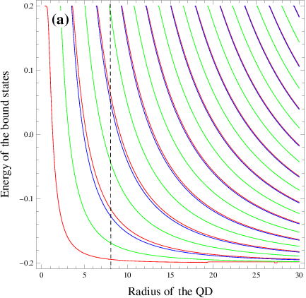
From the above computations we note that more bound states can be accommodated in the QD when the strength of the confining potential or the radius of the QD increase. These results are in agreement with previous work on bound state energies in radially symmetric graphene QD [8, 13]. In Figure 3 we show six bound states for V0=0.6V_{0}=0.6 and R=30R=30: two for j=12j=\frac{1}{2}, two for j=32j=\frac{3}{2} and two for j=52j=\frac{5}{2}.

Refer to caption

Refer to caption

Figure 3: (a): The contour plot of the energy of the bound states in a graphene quantum dot as a function of the radius RR. (b): The contour plot of the energy of the bound states in a graphene quantum dot as a function of the potential V0V_{0}. With j=12j=\frac{1}{2} (red line), j=32j=\frac{3}{2} (green line), j=52j=\frac{5}{2} (blue line), m=0.2m=0.2, and S0=1.6S_{0}=1.6. V0=0.6V_{0}=0.6 for (a), R=30R=30 for (b).
Refer to caption

Refer to caption

Figure 4: (a): The contour plot of the energy of the bound states in a graphene quantum dot as a function of the radius RR. (b): The contour plot of the energy of the bound states in a graphene quantum dot as a function of the potential S0S_{0}. With j=12j=\frac{1}{2} (red line), j=32j=\frac{3}{2} (green line), j=52j=\frac{5}{2} (blue line), m=0.2m=0.2, and S0=1.5S_{0}=1.5 for (a), R=8R=8 for (b).

At this stage, let us consider the case of spin symmetric configuration with V=SV=S. Within the framework of the Dirac equation, this configuration occurs when the difference between the Lorentz vector potential V⁡(r)V(r) and the Lorentz scalar potential S⁡(r)S(r) is constant, that is, Δ⁡(r)=V⁡(r)−S⁡(r)=constant\Delta(r)=V(r)-S(r)=\mbox{constant}, which in our case this constant is taken to be zero. The near experimental realization of the spin symmetric potential configuration may explain the degeneracy in some heavy meson spectra [18]. In this case (38) becomes

m−ε​Jj−12​(α​R)​Kj+12​(η​R)−ε−(m+2​S0)​Jj+12​(α​R)​Kj−12​(η​R​j)=0.\sqrt{m-\varepsilon}J_{j-\frac{1}{2}}(\alpha R)K_{j+\frac{1}{2}}(\eta R)-\sqrt{\varepsilon-(m+2S_{0})}J_{j+\frac{1}{2}}(\alpha R)K_{j-\frac{1}{2}}(\eta Rj)=0. (39)

Similarly to what we have seen in (38), (39) is also symmetric with respect to the transformation j→−jj\rightarrow-j.

In Figure 4 we show the solution of the equation (39). We note that when R=8R=8 and S0=1.6S_{0}=1.6 we have eight bound states: three for j=12j=\frac{1}{2}, three for j=32j=\frac{3}{2} and two for j=52j=\frac{5}{2}. We can also show that when we increase the radius of the dot or the strength of the pseudo scalar potential we accommodate more bound states.

4.2 Specific potential configuration

We consider the first configuration discussed in section 3 and study graphene in the presence of a mass term mm that induces a gap of value 2​m2m. The solution of the Dirac equation in this case is given in terms of the Whittaker hypergeometric functions Mν,μ±​(2​γ​r)M_{\nu,\mu_{\pm}}(2\gamma r) and Wν,μ±​(2​γ​r)W_{\nu,\mu_{\pm}}(2\gamma r), such as

Ψ⁡(r,θ)=∑k,±1r​ei2​(k−σ3)​θ​[𝒜±​Mν,μ±​(2​γ​r)+ℬ±​Wν,μ±​(2​γ​r)]\Psi(r,\theta)=\sum_{k,\pm}\frac{1}{\sqrt{r}}e^{\frac{i}{2}(k-\sigma_{3})\theta}[{\rm{\mathcal{A}_{\pm}}}M_{\nu,\mu_{\pm}}(2\gamma r)+{\rm{\mathcal{B}_{\pm}}}W_{\nu,\mu_{\pm}}(2\gamma r)] (40)

where Mν,μ±​(2​γ​r)M_{\nu,\mu_{\pm}}(2\gamma r) and Wν,μ±​(2​γ​r)W_{\nu,\mu_{\pm}}(2\gamma r) are given in terms of confluent hypergeometric functions [16]

Mν,μ±​(2​γ​r)=e−γ​r​(2​γ​r)μ±+1/2​F11​(12+μ±−ν,1+2​μ±,2​γ​r)\displaystyle M_{\nu,\mu_{\pm}}(2\gamma r)=e^{-\gamma r}(2\gamma r)^{{\mu_{\pm}}+1/2}{}_{1}F_{1}\left(\frac{1}{2}+\mu_{\pm}-\nu,1+2\mu_{\pm},2\gamma r\right) (41)
Wν,μ±​(2​γ​r)=e−γ​r​(2​γ​r)μ±+1/2​U​(12+μ±−ν,1+2​μ±,2​γ​r).\displaystyle W_{\nu,\mu_{\pm}}(2\gamma r)=e^{-\gamma r}(2\gamma r)^{\mu_{\pm}+1/2}U\left(\frac{1}{2}+\mu_{\pm}-\nu,1+2\mu_{\pm},2\gamma r\right). (42)

Then, the general solution, that is regular at the origin and decays exponentially at large rr, can be written in terms of the confluent hypergeometric function as

(2​γ)μ±+12​e−γ​r​rμ±​{𝒜±​F11​(12+μ±−ν,1+2​μ±,2​γ​r),r<Rℬ±​U​(12+μ±−ν,1+2​μ±,2​γ​r),r>R(2\gamma)^{\mu_{\pm}+\frac{1}{2}}e^{-\gamma r}r^{\mu_{\pm}}\left\{\begin{array}[]{lll}{{\rm{\mathcal{A}_{\pm}}}\ {}_{1}F_{1}\left(\frac{1}{2}+\mu_{\pm}-\nu,1+2\mu_{\pm},2\gamma r\right),}&&{r<R}\\ {{\rm{\mathcal{B}_{\pm}}}\ U\left(\frac{1}{2}+\mu_{\pm}-\nu,1+2\mu_{\pm},2\gamma r\right),}&&{r>R}\end{array}\right. (43)

where μ±=j∓12\mu_{\pm}=j\mp\frac{1}{2}, ν=−Wγ​j\nu=-\frac{W}{\gamma}j and γ2=(m+S)2+W2−(ε−e​V)2\gamma^{2}=\left(m+S\right)^{2}+W^{2}-\left(\varepsilon-eV\right)^{2}.

At this stage let us investigate the bound states. For this purpose, we adopt the explicit potential configuration

V⁡(r)={V0r<R0r>R,W⁡(r)={W0r<R0r>R,S⁡(r)={S0r<R0r>RV(r)=\left\{\begin{array}[]{lll}{V_{0}}&&{r<R}\\ {0}&&{r>R}\end{array}\right.,\qquad W(r)=\left\{\begin{array}[]{lll}{W_{0}}&&{r<R}\\ {0}&&{r>R}\end{array}\right.,\qquad S(r)=\left\{\begin{array}[]{lll}{S_{0}}&&{r<R}\\ {0}&&{r>R}\end{array}\right. (44)

which will help us simplify the above established formalism. The two matching conditions of the spinors at r=Rr=R give

γje−γ​R𝒜+F11(j−ν,2j,2γR)=γ′je−γ′Rℬ+U(j,2j,2γ′R)\displaystyle\gamma^{j}e^{-\gamma R}{\rm{\mathcal{A}_{+}}}\ {{}_{1}F_{1}}(j-\nu,2j,2\gamma R)={\gamma^{\prime}}^{j}e^{-\gamma^{{}^{\prime}}R}{\rm{\mathcal{B}_{+}}}\ U(j,2j,2\gamma^{{}^{\prime}}R) (45)
γj+1e−γ​R𝒜−F11(j+1−ν,2(j+1),2γR)=γ′j+1e−γ′Rℬ−U(j+1,2(j+1),2γ′R).\displaystyle\gamma^{j+1}e^{-\gamma R}{\rm{\mathcal{A}_{-}}}\ {{}_{1}F_{1}}(j+1-\nu,2(j+1),2\gamma R)={\gamma^{\prime}}^{j+1}e^{-\gamma^{{}^{\prime}}R}{\rm{\mathcal{B}_{-}}}\ U(j+1,2(j+1),2\gamma^{{}^{\prime}}R). (46)

Now inside and outside the QD we have, respectively, the quantities γ2=(m+S0)2+W02−(ε−V0)2\gamma^{2}=\left(m+S_{0}\right)^{2}+W_{0}^{2}-\left(\varepsilon-V_{0}\right)^{2} and γ2′=m2−ε2\gamma^{{}^{\prime}2}=m^{2}-\varepsilon^{2}. The condition for the existence of the bound states can be written as follows

γ′𝒜+𝒜−F11​(j−ν,2​j,2​γ​R)F11​(j+1−ν,2​(j+1),2​γ​R)=γℬ+ℬ−U(j,2j,2γ′R)U(j+1,2(j+1),2γ′R)\gamma^{{}^{\prime}}\frac{{\rm{\mathcal{A}_{+}}}}{{\rm{\mathcal{A}_{-}}}}\frac{{{}_{1}F_{1}}(j-\nu,2j,2\gamma R)}{{{}_{1}F_{1}}(j+1-\nu,2(j+1),2\gamma R)}=\gamma\frac{{\rm{\mathcal{B}_{+}}}}{{\rm{\mathcal{B}_{-}}}}\frac{U(j,2j,2\gamma^{{}^{\prime}}R)}{U(j+1,2(j+1),2\gamma^{{}^{\prime}}R)} (47)

where the ratios 𝒜+𝒜−\frac{{\rm{\mathcal{A}_{+}}}}{{\rm{\mathcal{A}_{-}}}} and ℬ+ℬ−\frac{{\rm{\mathcal{B}_{+}}}}{{\rm{\mathcal{B}_{-}}}} are fixed by the coupled differential equation (17) using the general solutions for r<Rr<R and r>Rr>R. After a straightforward but lengthy algebra we obtain

𝒜+𝒜−=−2​(m+S0)2+W02+(ε−V0)2m+S0−ε+V0​(2​j+1),ℬ+ℬ−=m+εm−ε\frac{{\rm{\mathcal{A}_{+}}}}{{\rm{\mathcal{A}_{-}}}}=-2\frac{\sqrt{(m+S_{0})^{2}+W_{0}^{2}+(\varepsilon-V_{0})^{2}}}{m+S_{0}-\varepsilon+V_{0}}(2j+1),\qquad\frac{{\rm{\mathcal{B}_{+}}}}{{\rm{\mathcal{B}_{-}}}}=\frac{\sqrt{m+\varepsilon}}{\sqrt{m-\varepsilon}} (48)

and (47) becomes

ξF11(j−ν,2j,2γR)U(j+1,2(j+1),2γ′R)+ζF11(j+1−ν,2(j+1),2γR)U(j,2j,2γ′R)=0\xi{{}_{1}F_{1}}(j-\nu,2j,2\gamma R)U(j+1,2(j+1),2\gamma^{{}^{\prime}}R)+\zeta{{}_{1}F_{1}}(j+1-\nu,2(j+1),2\gamma R)U(j,2j,2\gamma^{{}^{\prime}}R)=0 (49)

where ξ=2​(2​j+1)​(m−ε)\xi=2(2j+1)(m-\varepsilon), ζ=(m+S0−(ε−V0))\zeta=(m+S_{0}-(\varepsilon-V_{0})), γ=(m+S0)2+W02−(ε−V0)2\gamma=\sqrt{(m+S_{0})^{2}+W_{0}^{2}-(\varepsilon-V_{0})^{2}}, γ′=m2−ε2\gamma^{{}^{\prime}}=\sqrt{m^{2}-\varepsilon^{2}} and ν=−W0γ​j\nu=-\frac{W_{0}}{\gamma}j.

Refer to caption

Refer to caption

Figure 5: The contour plot of the energy of the bound states in a graphene quantum dots as a function of the radius RR of the quantum dot with j=12j=\frac{1}{2}, j=32j=\frac{3}{2}, j=52j=\frac{5}{2}, m=0.6m=0.6, S0=0.2S_{0}=0.2, V0=1.6V_{0}=1.6 and W0=0W_{0}=0 for (a), W0=0.5W_{0}=0.5 for (b)

In Figure 5 we show the energy of the QD as a function of the dot radius RR. Evaluating 49, we show the states only for j=12,32,52j=\frac{1}{2},\frac{3}{2},\frac{5}{2}. We use m=0.6m=0.6, V0=1.6V_{0}=1.6, S0=0.2S_{0}=0.2 and W0=0W_{0}=0 in Figure 5a, W0=0.5W_{0}=0.5 in Figure 5b. We can clearly see the effect of the pseud-scalar potential, its presence leads to the reduction of the number of the bound states. In the situation where W0=0W_{0}=0 and R=5R=5 we have eight bounds states: three with j=12j=\frac{1}{2}, three with j=32j=\frac{3}{2} and two with j=52j=\frac{5}{2}. On the other hand, for W0=0.5W_{0}=0.5 and for the same value of RR (R=5)(R=5), we have only seven bounds states: three with j=12j=\frac{1}{2}, two with j=32j=\frac{3}{2} and two with j=52j=\frac{5}{2}. From Figure 5 it is clearly seen that when we increase the radius of the QD more bound state can be accommodated in the QD, the same remark was made for the first potential configuration. The presence of a pseud-scalar potential leads to the reduction of the number of the bounds states.

Refer to caption

Refer to caption

Figure 6: The contour plot of the energy of the bound states in a graphene quantum dots as a function of the potential S0S_{0} with j=12j=\frac{1}{2}, j=32j=\frac{3}{2}, j=52j=\frac{5}{2}, m=0.6m=0.6, S0=0.2S_{0}=0.2, R=5R=5 and W0=0W_{0}=0 for (a), W0=0.5W_{0}=0.5 for (b).

In Figure 6 we show the evolution of the energy of the bound states as function of the strength of the potential V0V_{0}. Similarly to Figure 5, we present only the states with j=12,32,52j=\frac{1}{2},\frac{3}{2},\frac{5}{2}. We use m=0.6m=0.6, S0=0.2S_{0}=0.2, R=5R=5 and W0=0W_{0}=0 in Figure 6a and W0=0.5W_{0}=0.5 in Figure 6b. We note that when V0=1.6V_{0}=1.6 and W0=0W_{0}=0 we have eight bounds states: three with j=12j=\frac{1}{2}, three with j=32j=\frac{3}{2} and two with j=52j=\frac{5}{2}. On the other hand when W0=0.5W_{0}=0.5, for the same V0=1.6V_{0}=1.6 we only have seven bounds states: three with j=12j=\frac{1}{2}, two with j=32j=\frac{3}{2} and two with j=52j=\frac{5}{2}. These results are is in good agreement with Figure 5. It is clearly seen from Figure 6 that when we increase the radius of the QD we can accommodate more bound states like in the first case. In conclusion, the presence of a pseud-scalar potential leads to the reduction of the number of the bound states.

5 Transport properties of graphene quantum dot

In order to calculate the transport properties through a circular graphene quantum dot, we consider the spin symmetric potential configuration with V=SV=S and use a radially symmetric potential profile

S⁡(r)={U,r<a0,a<r<bS,b<r.S(r)=\left\{\begin{array}[]{lll}{U,}&&{r<a}\\ {0,}&&{a<r<b}\\ {S,}&&{b<r.}\end{array}\right. (50)

This potential represents a quantum dot of radius aa connected to an environment represented by the external region r>br>b. Bound states of the quantum dot are allowed to leak through the junction region, a<r<ba<r<b, to reach the environment at r>br>b. The general solution of the Dirac equation is oscillatory for r<ar<a and decays exponentially for b<rb<r, so that we can have incoming and outgoing waves in the intermediate region (a<r<ba<r<b) and define a scattering cross section. The radial solutions of the Dirac equation are given by

{A±​Jν±​(β​r),r<aA1±​Kν±​(η​r)+B1±​Iν±​(η​r),a<r<bA2±​Hν±(1)​(α​r)+B2±​Hν±(2)​(α​r),b<r\left\{\begin{array}[]{lll}{A_{\pm}J_{\nu_{\pm}}(\beta r),}&&{r<a}\\ {A_{1\pm}K_{\nu_{\pm}}(\eta r)+B_{1\pm}I_{\nu_{\pm}}(\eta r),}&&{a<r<b}\\ {A_{2\pm}H^{(1)}_{\nu_{\pm}}(\alpha r)+B_{2\pm}H^{(2)}_{\nu_{\pm}}(\alpha r),}&&{b<r}\end{array}\right. (51)

where α=(ε−(m+2​S))​(m+ε)\alpha=\sqrt{(\varepsilon-(m+2S))(m+\varepsilon)}, η=m2−ε2\eta=\sqrt{m^{2}-\varepsilon^{2}} and β=(ε−(m+2​U))​(m+ε)\beta=\sqrt{(\varepsilon-(m+2U))(m+\varepsilon)}.

The Dirac equation, H​Ψ=ε​ΨH\Psi=\varepsilon\Psi, has a scattering solution and the corresponding asymptotic form can be written as [19]

Ψ⁡(r,θ)=Ψ𝗂𝗇​(r,θ)+Ψ𝗈𝗎𝗍​(r,θ)\Psi(r,\theta)=\Psi_{\sf in}(r,\theta)+\Psi_{\sf out}(r,\theta) (52)

where Ψ𝗂𝗇​(r,θ)\Psi_{\sf in}(r,\theta) is the incoming plane wave in the xx-direction and Ψ𝗈𝗎𝗍​(r,θ)\Psi_{\sf out}(r,\theta) is the scattered outgoing spherical wave. These solutions have asymptotic behavior as r→∞r\rightarrow\infty given by

Ψ𝗂𝗇​(r,θ)=12​ei​α​r​cos⁡θ​(m+εε−(m+2​S))\displaystyle\Psi_{\sf in}(r,\theta)=\frac{1}{\sqrt{2}}e^{i\alpha r\cos\theta}\begin{pmatrix}{\sqrt{m+\varepsilon}}\\ {\sqrt{\varepsilon-(m+2S)}}\\ \end{pmatrix} (53)
Ψ𝗈𝗎𝗍​(r,θ)=ei​α​rπ​α​r​f±​(θ)​(m+εε−(m+2​S))\displaystyle\Psi_{\sf out}(r,\theta)=\frac{e^{i\alpha r}}{\sqrt{\pi\alpha r}}f_{\pm}(\theta)\begin{pmatrix}{\sqrt{m+\varepsilon}}\\ {\sqrt{\varepsilon-(m+2S)}}\\ \end{pmatrix} (54)

where f⁡(θ)f(\theta) defines the scattering amplitude and θ\theta is the scattering angle. Next, we use the decomposition of the plane wave

ei​α​x=∑m=−∞∞im​Jm​(k2​r)​ei​m​θe^{i\alpha x}=\sum\limits_{m=-\infty}^{\infty}i^{m}J_{m}(k_{2}r)e^{im\theta} (55)

and the asymptotic forms of the Bessel functions at large rr

Jm​(α​r)≈12​π​α​r​(ei⁡(α​r−m2​π−π4)+e−i⁡(α​r−m2​π−π4))\displaystyle J_{m}(\alpha r)\approx\frac{1}{\sqrt{2\pi\alpha r}}\left(e^{i(\alpha r-\frac{m}{2}\pi-\frac{\pi}{4})}+e^{-i(\alpha r-\frac{m}{2}\pi-\frac{\pi}{4})}\right) (56)
Hm(1,2)​(α​r)≈2π​α​r​e±i⁡(α​r−m2​π−π4).\displaystyle H^{(1,2)}_{m}(\alpha r)\approx\sqrt{\frac{2}{\pi\alpha r}}e^{\pm i\left(\alpha r-\frac{m}{2}\pi-\frac{\pi}{4}\right)}. (57)

In order to extract more information about the present system, let us study the differential and total cross sections. These are given by [19]

d​Λ​(θ)d​θ=|f⁡(θ)|22​π​α,Λ=∮|f⁡(θ)|22​π​α​𝑑θ.\frac{d\Lambda(\theta)}{d\theta}=\frac{|f(\theta)|^{2}}{2\pi\alpha},\qquad\Lambda=\oint\frac{|f(\theta)|^{2}}{2\pi\alpha}d\theta. (58)

where the scattering amplitude f±​(θ)f_{\pm}(\theta) can be expanded in Fourier series with coefficient fjf_{j}, such as

f±​(θ)=12​∑jei⁡((j∓12)−π4)​θ​fj.f_{\pm}(\theta)=\frac{1}{\sqrt{2}}\sum_{j}e^{i((j\mp\frac{1}{2})-\frac{\pi}{4})\theta}f_{j}. (59)

Combining all these results to write the asymptotic solutions as

Ψ±​(r,θ)=∑m=−∞∞im2​π​α​r​[(1+fj)​ei⁡(α​r−m​π2−π4)+e−i⁡(α​r−m​π2−π4)]​(m+Sε−(m+2​S))​ei​m​θ.\Psi_{\pm}(r,\theta)=\sum\limits_{m=-\infty}^{\infty}\frac{i^{m}}{\sqrt{2\pi\alpha r}}\left[\left(1+f_{j}\right)e^{i(\alpha r-\frac{m\pi}{2}-\frac{\pi}{4})}+e^{-i(\alpha r-\frac{m\pi}{2}-\frac{\pi}{4})}\right]\begin{pmatrix}{\sqrt{m+S}}\\ {\sqrt{\varepsilon-(m+2S)}}\\ \end{pmatrix}e^{im\theta}. (60)

Turning back to the solution in (51), the asymptotic form for the spinor wave function when b<rb<r can be expressed as

Φj​(r)≈2π​α​r​(A2±​ei⁡(α​r−m2​π−π4)+B2±​e−i⁡(α​r−m2​π−π4))\Phi_{j}(r)\approx\sqrt{\frac{2}{\pi\alpha r}}\left(A_{2\pm}e^{i(\alpha r-\frac{m}{2}\pi-\frac{\pi}{4})}+B_{2\pm}e^{-i(\alpha r-\frac{m}{2}\pi-\frac{\pi}{4})}\right) (61)

where the parameters are defined by

A2+=m+ε​Sj,A2−=ε−(m+2​S)​Sj\displaystyle A_{2+}=\sqrt{m+\varepsilon}S_{j},\qquad A_{2-}=\sqrt{\varepsilon-(m+2S)}S_{j} (62)
B2+=m+ε,B2−=ε−(m+2​S).\displaystyle B_{2+}=\sqrt{m+\varepsilon},\qquad B_{2-}=\sqrt{\varepsilon-(m+2S)}. (63)

We have defined the scattering matrix SjS_{j} by Sj=fj+1S_{j}=f_{j}+1. Applying the matching conditions at the boundaries r=ar=a and r=br=b we obtain

A+​Jj−12​(β​a)=A1+​Kj−12​(η​a)+B1+​Ij−12​(η​a)A−​Jj+12​(β​a)=A1−​Kj+12​(η​a)+B1−​Ij+12​(η​a)A1+​Kj−12​(η​b)+B1+​Ij−12​(η​b)=A2+​Hj−12(1)​(α​b)+B2+​Hj−12(2)​(α​b)A1−​Kj+12​(η​b)+B1−​Ij+12​(η​b)=A2−​Hj+12(1)​(α​b)+B2−​Hj+12(2)​(α​b)\displaystyle\begin{array}[]{lll}{A_{+}J_{j-\frac{1}{2}}(\beta a)}&=&{A_{1+}K_{j-\frac{1}{2}}(\eta a)+B_{1+}I_{j-\frac{1}{2}}(\eta a)}\\ {A_{-}J_{j+\frac{1}{2}}(\beta a)}&=&{A_{1-}K_{j+\frac{1}{2}}(\eta a)+B_{1-}I_{j+\frac{1}{2}}(\eta a)}\\ {A_{1+}K_{j-\frac{1}{2}}(\eta b)+B_{1+}I_{j-\frac{1}{2}}(\eta b)}&=&{A_{2+}H^{(1)}_{j-\frac{1}{2}}(\alpha b)+B_{2+}H^{(2)}_{j-\frac{1}{2}}(\alpha b)}\\ {A_{1-}K_{j+\frac{1}{2}}(\eta b)+B_{1-}I_{j+\frac{1}{2}}(\eta b)}&=&{A_{2-}H^{(1)}_{j+\frac{1}{2}}(\alpha b)+B_{2-}H^{(2)}_{j+\frac{1}{2}}(\alpha b)}\end{array}

The relationship between the different coefficients reads

A1+A1−=m+εm−ε,B1+B1−=−m+εm−ε,A+A−=m+εε−(m+2​U).\frac{A_{1+}}{A_{1-}}=\frac{\sqrt{m+\varepsilon}}{\sqrt{m-\varepsilon}},\qquad\frac{B_{1+}}{B_{1-}}=-\frac{\sqrt{m+\varepsilon}}{\sqrt{m-\varepsilon}},\qquad\frac{A_{+}}{A_{-}}=\frac{\sqrt{m+\varepsilon}}{\sqrt{\varepsilon-(m+2U)}}. (66)

Defining the matrix

M(1,2)=\displaystyle M^{(1,2)}= (67)
(−m+ε​Jj−12​(β​a)m+ε​Kj−12​(η​a)m+ε​Ij−12​(η​a)0−ε−(m+2​U)​Jj+12​(β​a)m−ε​Kj+12​(η​a)−m−ε​Ij+12​(η​a)00m+ε​Kj−12​(η​b)m+ε​Ij−12​(η​b)m+ε​Hj−12(1,2)​(α​b)0m−ε​Kj+12​(η​b)−m−ε​Ij+12​(η​b)ε−(m+2​S)​Hj+12(1,2)​(α​b))\displaystyle\begin{pmatrix}{-\sqrt{m+\varepsilon}J_{j-\frac{1}{2}}(\beta a)}&{\sqrt{m+\varepsilon}K_{j-\frac{1}{2}}(\eta a)}&{\sqrt{m+\varepsilon}I_{j-\frac{1}{2}}(\eta a)}&{0}\\ {-\sqrt{\varepsilon-(m+2U)}J_{j+\frac{1}{2}}(\beta a)}&{\sqrt{m-\varepsilon}K_{j+\frac{1}{2}}(\eta a)}&{-\sqrt{m-\varepsilon}I_{j+\frac{1}{2}}(\eta a)}&{0}\\ {0}&\sqrt{m+\varepsilon}K_{j-\frac{1}{2}}(\eta b)&{\sqrt{m+\varepsilon}I_{j-\frac{1}{2}}(\eta b)}&{\sqrt{m+\varepsilon}H^{(1,2)}_{j-\frac{1}{2}}(\alpha b)}\\ {0}&\sqrt{m-\varepsilon}K_{j+\frac{1}{2}}(\eta b)&{-\sqrt{m-\varepsilon}I_{j+\frac{1}{2}}(\eta b)}&{\sqrt{\varepsilon-(m+2S)}H^{(1,2)}_{j+\frac{1}{2}}(\alpha b)}\end{pmatrix}

After a straightforward algebra we obtain the scattering matrix as

Sj=−detM2detM1.S_{j}=-\frac{\det M^{2}}{\det M^{1}}. (68)
Refer to caption

Refer to caption

Figure 7: Angular dependence of the differential cross section, d​σ​(θ)/d​θd\sigma(\theta)/d\theta, in nanometers, for R=25​n​mR=25nm, L=80​n​mL=80nm, m=0.1​m​e​Vm=0.1meV and ε=5​m​e​V\varepsilon=5meV. In (a): the green line correspond to U=0.2​m​e​VU=0.2meV and the pseudo scalar potential S=0.2​m​e​VS=0.2meV. The red line correspond to U=0.2​m​e​VU=0.2meV ant S=0.8​m​e​VS=0.8meV. In (b): the blue line correspond to U=0.2​m​e​VU=0.2meV and S=0.8​m​e​VS=0.8meV. The orange line correspond to U=0.6​m​e​VU=0.6meV and S=0.8​m​e​VS=0.8meV.

In Figure 7 we show the angular dependence of the differential cross section. The differential cross section shows a narrow maximum at θ=0\theta=0 and has a zero minimum when θ=π/2\theta=\pi/2. In addition the differential cross section is no longer symmetric with respect to the sign of the incident angle. In Figure 7a, we fix SS at 0.20.2 and take two different values for UU, U=0.2U=0.2 correspond to the green curve and U=0.8U=0.8 correspond to the red one. One can see that the maximum value of the differential cross section increase when UU decrease to a value that is greater than 0.20.2. In Figure 7b, we fix S=0.8S=0.8 and take two different values of UU, the orange line correspond to U=0.2U=0.2 and the blue line correspond to U=0.8U=0.8. This shows that the maximum of the differential cross section increase when the value of UU increase even for values which are still smaller than 0.80.8.

6 Scattering through quantum dot

Below we develop the scattering theory for the 2D Dirac fermions in the presence of an axially symmetric potential using the second potential configuration. The Dirac equation, H​Ψ=E​ΨH\Psi=E\Psi, has scattering solutions that have the asymptotic form [19] Ψ⁡(r,θ)=Ψ𝗂𝗇​(r,θ)+Ψ𝗈𝗎𝗍​(r,θ)\Psi(r,\theta)=\Psi_{\sf in}(r,\theta)+\Psi_{\sf out}(r,\theta). These solutions have the following asymptotic forms as r→∞r\rightarrow\infty

Ψ𝗂𝗇​(r,θ)=12​ei​α​r​cos⁡θ​(11)\displaystyle\Psi_{\sf in}(r,\theta)=\frac{1}{\sqrt{2}}e^{i\alpha r\cos\theta}\begin{pmatrix}{1}\\ {1}\\ \end{pmatrix} (69)
Ψ𝗈𝗎𝗍​(r,θ)=ei​α​r−2​i​π​α​r​(f+​(θ)f−​(θ))\displaystyle\Psi_{\sf out}(r,\theta)=\frac{e^{i\alpha r}}{\sqrt{-2i\pi\alpha r}}\begin{pmatrix}{f_{+}(\theta)}\\ {f_{-}(\theta)}\\ \end{pmatrix} (70)

where Ψ𝗂𝗇​(r,θ)\Psi_{\sf in}(r,\theta) is the incoming plane wave in the xx-direction and Ψ𝗈𝗎𝗍​(r,θ)\Psi_{\sf out}(r,\theta) is the scattered outgoing spherical wave, f±​(θ)f_{\pm}(\theta) is the scattering amplitude and θ\theta is the scattering angle, furthermore, f−​(θ)=ei​θ​f+​(θ)f_{-}(\theta)=e^{i\theta}f_{+}(\theta). The incoming particle current density is α\alpha. The number of particles leaving per unit time radially in the direction θ\theta is d​θπ​|f⁡(θ)|2\frac{d\theta}{\pi}|f(\theta)|^{2}. Thus the differential scattering cross section is

d​σ​(θ)d​θ=|f⁡(θ)|2π​α.\frac{d\sigma(\theta)}{d\theta}=\frac{|f(\theta)|^{2}}{\pi\alpha}. (71)

For large rr, the solution of the Dirac equation is given as a function of the Hankel functions of the first and second kind, Hμ(1,2)​(α​r)=Jμ​(α​r)±i​Yμ​(α​r)H^{(1,2)}_{\mu}(\alpha r)=J_{\mu}(\alpha r)\pm iY_{\mu}(\alpha r), where the upper sign holds for the superscript 1 and the lower one for 2. Their asymptotic behavior when α​r→∞\alpha r\rightarrow\infty is given by

Jμ​(α​r)≈2π​α​r​cos⁡(α​r−(2​μ+1)4​π)\displaystyle J_{\mu}(\alpha r)\approx\sqrt{\frac{2}{\pi\alpha r}}\cos\left(\alpha r-\frac{(2\mu+1)}{4}\pi\right) (72)
Yμ​(α​r)≈2π​α​r​sin⁡(α​r−(2​μ+1)4​π)\displaystyle Y_{\mu}(\alpha r)\approx\sqrt{\frac{2}{\pi\alpha r}}\sin\left(\alpha r-\frac{(2\mu+1)}{4}\pi\right) (73)
Hμ(1,2)​(α​r)≈2π​α​r​e±i⁡(α​r−(2​μ+1)4​π).\displaystyle H^{(1,2)}_{\mu}(\alpha r)\approx\sqrt{\frac{2}{\pi\alpha r}}e^{\pm i\left(\alpha r-\frac{(2\mu+1)}{4}\pi\right)}. (74)

We note that Ψ𝗈𝗎𝗍\Psi_{\sf out} for r→∞r\rightarrow\infty indeed has the form of (74). Using the decomposition of the plane wave [20]

ei​α​r​cos⁡θ=∑ji(j∓12)​ei⁡(j∓12)​θ​Jj∓12​(α​r)e^{i\alpha r\cos\theta}=\sum_{j}i^{(j\mp\frac{1}{2})}e^{i(j\mp\frac{1}{2})\theta}J_{j\mp\frac{1}{2}}(\alpha r) (75)

gives for the incoming wave

Ψ𝗂𝗇=(∑ji(j−12)​Jj−12​(α​r)​ei⁡(j−12)​θ∑ji(j+12)​Jj+12​(α​r)​ei⁡(j+12)​θ).\Psi_{\sf in}=\left(\begin{array}[]{c}\sum_{j}i^{(j-\frac{1}{2})}J_{j-\frac{1}{2}}\left(\alpha r\right)e^{i(j-\frac{1}{2})\theta}\\ \sum_{j}i^{(j+\frac{1}{2})}J_{j+\frac{1}{2}}\left(\alpha r\right)e^{i(j+\frac{1}{2})\theta}\\ \end{array}\right). (76)

We use the defining equation

f⁡(θ)=12​∑jfj​ei⁡(j∓12)​θ−i​π4f(\theta)=\frac{1}{\sqrt{2}}\sum_{j}f_{j}e^{i(j\mp\frac{1}{2})\theta-i\frac{\pi}{4}} (77)

so that the outgoing wave function when α​r→∞\alpha r\rightarrow\infty has the following form

Ψ𝗈𝗎𝗍=(∑ji(j−12)​fj​[Jj−12​(α​r)+i​Yj−12​(α​r)]​ei⁡(j−12)​θ∑ji(j+12)​fj​[Jj+12​(α​r)+i​Yj+12​(α​r)]​ei⁡(j+12)​θ).\Psi_{\sf out}=\left(\begin{array}[]{c}\sum_{j}i^{(j-\frac{1}{2})}f_{j}\left[J_{j-\frac{1}{2}}\left(\alpha r\right)+iY_{j-\frac{1}{2}}\left(\alpha r\right)\right]e^{i(j-\frac{1}{2})\theta}\\ \sum_{j}i^{(j+\frac{1}{2})}f_{j}\left[J_{j+\frac{1}{2}}\left(\alpha r\right)+iY_{j+\frac{1}{2}}\left(\alpha r\right)\right]e^{i(j+\frac{1}{2})\theta}\\ \end{array}\right). (78)

We assume that the scattering defect has a finite radius RR, so, when r>Rr>R we can write the wave functions as a superposition of terms such as

Ψj=([Jj−12​(α​r)+Rj​Yj−12​(α​r)]​ei⁡(j−12)​θi⁡[Jj+12​(α​r)+Rj​Yj+12​(α​r)]​ei⁡(j+12)​θ)\Psi_{j}=\left(\begin{array}[]{c}\left[J_{j-\frac{1}{2}}\left(\alpha r\right)+R_{j}Y_{j-\frac{1}{2}}\left(\alpha r\right)\right]e^{i(j-\frac{1}{2})\theta}\\ i\left[J_{j+\frac{1}{2}}\left(\alpha r\right)+R_{j}Y_{j+\frac{1}{2}}\left(\alpha r\right)\right]e^{i(j+\frac{1}{2})\theta}\\ \end{array}\right) (79)

where RjR_{j} is the reflection coefficients and the complex number ii is introduced for further convenience. From (76), (78) and (79) we can write

Ψ𝗂𝗇+Ψ𝗈𝗎𝗍=∑jβj​Ψj\Psi_{\sf in}+\Psi_{\sf out}=\sum_{j}\beta_{j}\Psi_{j} (80)

and one can deduce the expression of fjf_{j}

fj=Rji−Rj.f_{j}=\frac{R_{j}}{i-R_{j}}. (81)

The expression of the scattering amplitude can then be written in compact form

f⁡(θ)=∑jRji−Rj​ei⁡(j∓12)​θ−i​π4.f(\theta)=\sum_{j}\frac{R_{j}}{i-R_{j}}e^{i(j\mp\frac{1}{2})\theta-i\frac{\pi}{4}}. (82)

We note that the back-scattering amplitude vanishes, f⁡(π)=0f(\pi)=0, which is a consequence of the pseudospin conservation for chiral scattering [21] and is related to the Klein paradox [22].

Now we consider a circular potential barrier in graphene and choose V⁡(r)=V0​Θ​(R−r)V(r)=V_{0}\Theta(R-r) and S⁡(r)=S0​Θ​(R−r)S(r)=S_{0}\Theta(R-r) where Θ\Theta is the heaviside step function. Using the boundary conditions, continuity of the eigenspinors at r=Rr=R, we obtain

Jj−12​(α​R)+Rj​Yj−12​(α​R)=Tj​Jj−12​(α′​R)\displaystyle{J_{j-\frac{1}{2}}\left(\alpha R\right)+R_{j}Y_{j-\frac{1}{2}}\left(\alpha R\right)=T_{j}J_{j-\frac{1}{2}}\left(\alpha^{\prime}R\right)} (83)
Jj+12​(α​R)+Rj​Yj+12​(α​R)=Tj​Jj+12​(α′​R)\displaystyle{J_{j+\frac{1}{2}}\left(\alpha R\right)+R_{j}Y_{j+\frac{1}{2}}\left(\alpha R\right)=T_{j}J_{j+\frac{1}{2}}\left(\alpha^{\prime}R\right)} (84)

where α=(ε−V0)2−(Δ+S0)2\alpha=\sqrt{\left(\varepsilon-V_{0}\right)^{2}-\left(\Delta+S_{0}\right)^{2}} and α′=ε2−Δ2\alpha^{\prime}=\sqrt{\varepsilon^{2}-\Delta^{2}}. The reflection coefficient is then given by

Rj=−Jj−12​(α​R)​Jj+12​(α′​R)−Jj+12​(α​R)​Jj−12​(α′​R)Yj−12​(α​R)​Jj+12​(α′​R)−Yj+12​(α​R)​Jj−12​(α′​R).R_{j}=-\frac{J_{j-\frac{1}{2}}\left(\alpha R\right)J_{j+\frac{1}{2}}\left(\alpha^{\prime}R\right)-J_{j+\frac{1}{2}}\left(\alpha R\right)J_{j-\frac{1}{2}}\left(\alpha^{\prime}R\right)}{Y_{j-\frac{1}{2}}\left(\alpha R\right)J_{j+\frac{1}{2}}\left(\alpha^{\prime}R\right)-Y_{j+\frac{1}{2}}\left(\alpha R\right)J_{j-\frac{1}{2}}\left(\alpha^{\prime}R\right)}. (85)

Similarly for the transmission coefficient

Tj=Yj+12​(α​R)​Jj−12​(α​R)−Yj−12​(α​R)​Jj+12​(α​R)Yj+12​(α​R)​Jj−12​(α′​R)−Yj−12​(α​R)​Jj+12​(α′​R).T_{j}=\frac{Y_{j+\frac{1}{2}}\left(\alpha R\right)J_{j-\frac{1}{2}}\left(\alpha R\right)-Y_{j-\frac{1}{2}}\left(\alpha R\right)J_{j+\frac{1}{2}}\left(\alpha R\right)}{Y_{j+\frac{1}{2}}\left(\alpha R\right)J_{j-\frac{1}{2}}\left(\alpha^{\prime}R\right)-Y_{j-\frac{1}{2}}\left(\alpha R\right)J_{j+\frac{1}{2}}\left(\alpha^{\prime}R\right)}. (86)

We have the relations J−n​(x)=(−1)n​Jn​(x)J_{-n}(x)=(-1)^{n}J_{n}(x) and Y−n​(x)=(−1)n​Yn​(x)Y_{-n}(x)=(-1)^{n}Y_{n}(x) [20]. If we take n=j−12n=j-\frac{1}{2}, nn is an integer, we get Rn=R−n−1R_{n}=R_{-n-1}, so the back-scattering amplitude vanishes, and Tn=T−n−1T_{n}=T_{-n-1}, that is n↔−n−1n\leftrightarrow-n-1 which means fn=f−n−1f_{n}=f_{-n-1}. Thus, (71) can be rewritten in a compact form

d​σ​(θ)d​θ=1π​α​|∑n=0∞fn​cos⁡(n+12)​θ|2.\frac{d\sigma(\theta)}{d\theta}=\frac{1}{\pi\alpha}\left|\sum_{n=0}^{\infty}f_{n}\cos{(n+\frac{1}{2})\theta}\right|^{2}. (87)

The angular dependence of the cross section is shown in Figure 8, where we have the cross section as a function of the incident angle θ\theta which shows a narrow maximum at θ=0\theta=0.

Refer to caption
Figure 8: Angular dependence of the differential cross section, d​σ​(θ)/d​θd\sigma(\theta)/d\theta, in nanometers, for the radius R=15​n​mR=15nm with the vector potential V0=40​m​e​VV_{0}=40meV. The green line correspond to ε=20​m​e​V\varepsilon=20meV, the pseudo scalar potential S0=8​m​e​VS_{0}=8meV and with the mass term m=7​m​e​Vm=7meV. The red line correspond to ε=15​m​e​V\varepsilon=15meV, S0=5​m​e​VS_{0}=5meV and with the mass term m=2.5​m​e​Vm=2.5meV

In Figure (8) we plot the dependence of the differential cross section on the incident angle θ\theta choosing different values of the parameters. We show that the curve is symmetric about the axis θ=0\theta=0. In addition, it is clearly seen that the differential cross section exhibits a narrow maximum around θ=0\theta=0 and vanishes when θ\theta goes to ±π\pm\pi. The differential cross section shows resonances associated with the QD quasi-bound states [21].

7 Conclusion

We studied the Dirac equation in (2+1)(2+1)-dimensions where we included all types of potential couplings: vector, pseudo-scalar and scalar. We used the method of separation of variables in polar coordinates to obtain the general spinor eigenfunctions and associated energy spectra for two special potential configurations. We have studied the bound states of graphene QD which can be created electrostatically in presence of a constant mass term. We discussed the character of the electronic eigenstates occurring in various regions of energy and potential parameters.

We used the solution of the Dirac equation for two potential configurations and studied the dependence of the electronic bound states on the strength of the electrostatic potential and the radius of the QD. For both potential configurations we showed that when we increase the radius of the QD or the strength of the confining potential more bound states can be accommodated in the QD, in agreement with usual quantum mechanical results.

We developed the scattering theory for the 2D Dirac fermions in the presence of the axially symmetric potential and computed the differential cross section. This differential cross section is associated with a quantum dot embedded in an environment. We showed that it is no longer symmetric with respect to the sign of the incident angle, it has a maximum around θ=0\theta=0 and exhibits resonances associated with quantum dot quasi-bound states. We also found that the variation of the potential strength changes the maximum of the differential cross section.

Acknowledgments

The generous support provided by the Saudi Center for Theoretical Physics (SCTP) is highly appreciated by all authors. AJ and HB acknowledges partial support by King Fahd University of Petroleum and minerals under the theoretical physics research group project RG1306-1 and RG1306-2.

References

  • [1] K. S. Novoselov, A. K. Geim, S. V. Morozov, D. Jiang, Y. Zhang, S. V. Dubonos, I. V. Grigorieva and A. A. Firsov, Science 306, 666 (2004).
  • [2] K. S. Novoselov, D. Jiang, T. Booth, V. V. Khotkevich, S. M. Morozov and A. K. Geim Proc. Natl Acad. Sci. 102 10451 (2005).
  • [3] A. K. Geim and K. S. Novoselov, Nature Materials 6, 183 (2007).
  • [4] T. Chakraborty, Quantum Dots (Elsevier, Amsterdam, 1999).
  • [5] P. G. Silvestrov and K. B. Efetov, Phys. Rev. Lett. 98, 016802 (2007).
  • [6] A. Matulis and F. M. Peeters, Phys. Rev. B 77, 115423 (2008).
  • [7] F. Guinea, J. Low Temp. Phys. 153, 359 (2008).
  • [8] G. Pal, W. Apel, and L. Schweitzer, Phys. Rev. B 84, 075446 (2011).
  • [9] H. Bahlouli, A. Jellal and Y. Zahidi, Int. J. Geo. Meth. Mod. Phys. 11, 1450036 (2014).
  • [10] V. B. Berestetskii, E. M. Lifshits and L. P. Pitaevskii, Quantum Electrodynamics (Elsevier, Oxford, 1971).
  • [11] M. Katsnelson and K. Novoselov, Solid State Commun. 143, 3 (2007).
  • [12] S. Y. Zhou, G. H. Gweon, A. V. Fedorov, P. N. First, W. A. deHeer, D. H. Lee, F. Guinea, A. H. Castro Neto and A. Lanzara, Nat. Mater 6, 770 (2007).
  • [13] P. Recher, J. Nilsson, G. Burkard and B. Trauzettel, Phys. Rev. B 79, 085407 (2009).
  • [14] A. De Martino, L. DellAnna and R. Egger, Phys. Rev. Lett. 98,066802 (2007).
  • [15] A. Jellal, A. D. Alhaidari and H. Bahlouli, Phys. Rev. A 80, 012109 (2009).
  • [16] M. Abramowitz and I. A. Stegun, Handbook of Mathematical Functions with Formulas, Graphs, and Mathematical Tables (New York: Dover Publications, 1972, p. 505).
  • [17] G. Giovannetti, P. A. Khomyakov, G. Brocks, P. J. Kelly and J. van den Brink, Phys. Rev. B 76, 073103 (2007).
  • [18] P. R. Page, T. Goldman and J. N. Ginocchio, Phys. Rev. Lett. 86, 204 (2001).
  • [19] L. D. Landau and E. M. Lifshits, Quantum Mechanics (Nonrelativistic Theory) (Elsevier, Oxford, 1977).
  • [20] I. S. Gradshteyn and I. M. Ryzhik. Table of Integrals, Series, and Products. Edited by A. Jeffrey and D. Zwillinger (Academic Press, New York, 7th edition, 2007).
  • [21] M. I. Katsnelson, F. Guinea and A. K. Geim, Phys. Rev. B 79, 195426 (2009).
  • [22] M. I. Katsnelson, K. S. Novoselov and A. K. Geim, Nat. Phys. 2, 620 (2006).