Epidemics and Cascade Dynamics on Heterogeneous Networks Complex systems Critical point phenomena Statistical physics and nonlinear dynamics
Dynamic Behavior of Interacting between Epidemics and Cascades on Heterogeneous Networks
Abstract
Epidemic spreading and cascading failure are two important dynamical processes over complex networks. They have been investigated separately for a long history. But in the real world, these two dynamics sometimes may interact with each other. In this paper, we explore a model combined with SIR epidemic spreading model and local loads sharing cascading failure model. There exists a critical value of tolerance parameter that whether the epidemic with high infection probability can spread out and infect a fraction of the network in this model. When the tolerance parameter is smaller than the critical value, cascading failure cuts off abundant of paths and blocks the spreading of epidemic locally. While the tolerance parameter is larger than the critical value, epidemic spreads out and infects a fraction of the network. A method for estimating the critical value is proposed. In simulation, we verify the effectiveness of this method in Barabási-Albert (BA) networks.
pacs
89.75.-kpacs
05.70.Jkpacs
05.10.-a1 Introduction
Epidemic spreading and cascading failure are extensively investigated in the research of complex networks. Study of epidemics on networks is an area of special interest including the spreading of infectious diseases, rumors [1] and computer viruses [2], and has deepened our insights into the interplay between topologies and the spreading dynamics [3, 4, 5, 6, 7]. Cascading failure is another phenomenon that random failures or intentional attacks lead to severe chain reactions propagating through links in networks. It is widely found in power transmission [8, 9], communication [10], economic [11], and biological [12] networks.
Traditionally, these two dynamics correspond to independent topics in the research of complex networks, i.e., when one of them is studied, the other is considered to be irrelevant. But in practice, there are many cases in which they interact with each other and neither of their effects can be ignored. For example, consider a digital virus spreading over a data communication network. In this scenario, an infected router may not deliver data packets normally and cause overloading of nearby routers. These routers then redistribute their loads to other routers. Eventually, a large cascading failure occurs. In turn, the cascading failure also influences the spreading of the virus, because failed nodes cannot deliver data properly, especially cannot deliver copies of the virus properly. A real-world case that computer viruses CODE RED and Nima caused widely reported BGP storms, which is a cascading failure, was observed in September of 2001 [13].
In our previous work [14], we proposed a model to study the interplay between epidemic spreading and cascading failure. In this model, when the two dynamical processes stop at equilibrium, the nodes both uninfected and un-failed form several clusters. We considered the relative size of the largest one, i.e. the giant component, and found that in both Erdös-Rényi (ER) random networks and BA scale free networks, with an infectivity over some threshold, a giant component forms only if the tolerance parameter , which captures the capacities of nodes, is within some interval . In Ref. [14], we have stated the reason for this – with under , a large-scale cascade occurs and almost all nodes fail, while with over , epidemics and cascading failure together kill almost all nodes.
In this paper, we explore this model from the perspective of epidemic spreading, while our previous work inspected it from the perspective of cascading failure. We consider the situation when the infection probability is sufficiently large. In this case, when is extremely small, the epidemic dies out locally since cascading failure cuts off almost all the paths in the network. When is sufficiently large, nodes will never be overloaded, epidemic thus can spreads out. Therefore, there exists a critical value that whether the epidemic with high infection probability can spread out. The critical value is different from in our previous work. The indicates the critical moment that epidemic starts to spread out but not die out locally, while implies the critical moment that epidemic and cascading failure kill all nodes in network together. In the rest of this paper, we devote our effort to further studying the interplay between epidemics and cascades, and pay special attention to the critical value .
2 Model
In Ref. [14], we link the epidemiological SIR model [15, 16] with a local load sharing cascading failure model together to form a hybrid model.
In the SIR model, nodes are in one of the three states: susceptible (S), infected (I), and removed (R). At every time step, the susceptible node becomes infected with probability for every link connecting an infected node with a susceptible node. The infected node becomes removed with probability . The effective spreading rate is . For simplicity, we let .
In our model, removed nodes in epidemic spreading are assumed to be not functioning and cannot manipulate loads. So the spreading of epidemic will lead to load redistribution, which may cause cascading failure in the network. We assume that the failed nodes in cascading failure are not functioning either, so they cannot infect or be infected by others. Because both removed and failed nodes no longer interact with other nodes in the consequent process, they are said to be inactive. All other nodes are said to be active.
Inspired by previous works [17, 18], we assume that when a node fails, a fixed positive load is transferred to each of its active neighbors. Overloaded nodes are those whose load exceeds their capacity. It is natural to assume that the capacity of a node is proportional to its initial load [19, 20, 21, 22]
| (1) |
where the constant is the tolerance parameter.
The numerical simulation of the hybrid process in an uncorrelated network with nodes is summarized as follows:
- 1.
The initial load of each node is randomly generated according to a uniform distribution on the interval [,] and its capacity is defined by Eq. (1). Without loss of generality, we let and .
- 2.
Randomly select a few nodes in the network as the initial infected nodes.
- 3.
For every link connecting an infected node with a susceptible node, the susceptible node becomes infected with probability , and for every infected node, it becomes removed with probability 1.
- 4.
The removal may cause load redistribution and possibly cascading failure. Repeat the cascades until there is no overloaded node in the network.
- 5.
If there exist infected nodes in the network, go back to 3 to start another step of epidemic spreading; otherwise, the process halts.
Note that we make another assumption that the time scale of cascading failure is much smaller than that of epidemic spreading, so every single step of epidemic spreading is executed until there are no overloaded nodes in the network.
3 Analysis


When the process ends at equilibrium, the active nodes in the network form several clusters. In Ref. [14], we use the fraction of the largest cluster, namely, the giant component, to measure the performance of the network. But here, for now, we examine the fraction of the active nodes rather than the largest cluster formed by them, because it is closely related to and more likely to be theoretically tractable. Fig. 1 shows as a function of the tolerance parameter in ER and BA networks. When is extremely small, cascading failure kills almost all nodes and epidemic dies out locally, thus is very close to zero. With increases, the severity of cascading failure reduces and increases. When is over some critical value, , the epidemic starts to spread out and infect a large number of nodes, making decrease.
3.1 Preliminaries
Before we introduce the method to solve the critical value in our model, we present some preliminary remarks.
The spread of disease is equivalent to a bond percolation process [23, 24]. With effective spreading rate , the equivalent process is as follows: select an edge from network with probability , and the outbreak of disease means that the set of chosen edges forms a connectivity cluster. The cascading failure is a site percolation process [25, 26]. There are several nodes participating in both bond percolation and site percolation processes. We assume that these nodes belong to site percolation process rather than bond percolation process. The reason for this assumption is that, although the cascading failure is triggered by the spreading of epidemic, once cascade starts with a small value of , most of the paths linked to infected nodes are cut off by cascading failure, and thus the number of failed nodes from cascading failure will be much larger than newly infected nodes. Therefore, most of the nodes participating in both bond percolation and site percolation processes are considered to be failed in cascades eventually, rather than removed in epidemic spreading. Note that there is a premise that is small, which means most of the inactive nodes come from cascades while epidemic is restricted in a small scale, since the time scale of cascading failure is much smaller than that of epidemic spreading. Based on the assumption above, we define two types of excessive states to describe the dynamics before a node becomes inactive as shown in Fig. 2:
Quasi-infected node, a node at least one of whose edges participates in bond percolation process.
Quasi-failed node, a node takes part in site percolation process.
A quasi-failed node will fail in cascades undoubtedly, while quasi-infected node will become removed or failed in the end. Denote as the probability that a node of degree happens to be a quasi-failed node, and that it happens to be a quasi-infected node. Eventually, this node happens to be failed with probability , or be removed with probability .

Further more, in this model, we call a node:
An -vulnerable node, if and only if it has quasi-failed or quasi-infected neighbors, and it becomes inactive if all of the neighbors fail and share load with it.
A Vulnerable node, if it is an -vulnerable node, where .
The probability that a node of degree happens to be a vulnerable node is
| (2) |
where is the probability that it is an -vulnerable node.
When is small, the number of quasi-failed nodes is larger than that of quasi-infected nodes, as the time scale of cascading failure is much smaller than that of epidemic spreading. Thus vulnerable nodes can be approximated to quasi-failed nodes, as .
3.2 Critical Value of Tolerance Parameter
In an uncorrelated network, consider a node of degree and any of its neighbor . The probability of node with degree is . Node becomes vulnerable or infected with probability . Therefore, the probability of node ’s arbitrary neighbor being quasi-failed or quasi-infected is
| (3) |
where and are the probabilities that node ’s arbitrary neighbor happens to be a failed or removed node at equilibrium, respectively, as follows,
| (4) | ||||
| (5) |
According to Eq. (3), the probability that exactly of node ’s neighbors are quasi-failed is
| (6) |
For node , its initial load is uniformly distributed in the range [0,1], so the cumulative distribution function of is
| (7) |
The probability that node ’s failure is triggered by the failure and loads sharing from exact of its neighbors is
| (8) |
Then, the probability that node is an -vulnerable node is
| (9) |
| (10) |
where is the floor function.
Eq. (10) provides the probability that arbitrary node in network turns out to be a quasi-failed node. Then, we will handle the probability of a node comes to be a quasi-infected node . We know the probability that node of degree survives with active state at equilibrium is . These nodes are active nodes, that they are neither quasi-failed nodes nor quasi-infected nodes. The state of these active nodes is determined by their neighbors:
- 1.
If their neighbors are quasi-failed or quasi-infected and finally become failed in cascades, then these active nodes may turn out to be failed as the overload caused by their neighbors. The probability of this situation happens is .
- 2.
If their neighbors are active nodes, i.e., the neighbors are neither quasi-failed nor quasi-infected nodes, then these active nodes will not fail. The probability of this situation happens is .
Thus the probability that a node survives with active state, , can be written follows its neighbors states as
| (11) |
In the first line of Eq. (11), indicates the situation that of node ’s neighbors are quasi-failed or quasi-infected nodes but it is still active. Based on the discussion above, we have , where is given in Eq. (10). According to Eq. (10) and Eq. (11), we can get
| (12) |
where is the probability that a node of degree be a removed node in epidemic spreading finally.
Now we complete the derivation by Eq. (4), (5), (10), (12). These four equations depend on each other. We can get , , the fraction of removed nodes , and the fraction of failed nodes at equilibrium from these four equations by the following iteration process:
- 1.
- 2.
- 3.
Get the fraction of removed and failed nodes at equilibrium by and respectively. With increases, the will change from zero to a positive value at and this indicates when the epidemic starts to spread out.
4 Simulations
We mainly focus on the fraction of active nodes in simulation, and validate the theoretical results of critical value . We carry out the simulations in BA networks with 5000 nodes and varied average degrees . The results are averaged over 50 realizations in each of which the network is independently generated. The unit of load shared in cascading failure, , is fixed at .
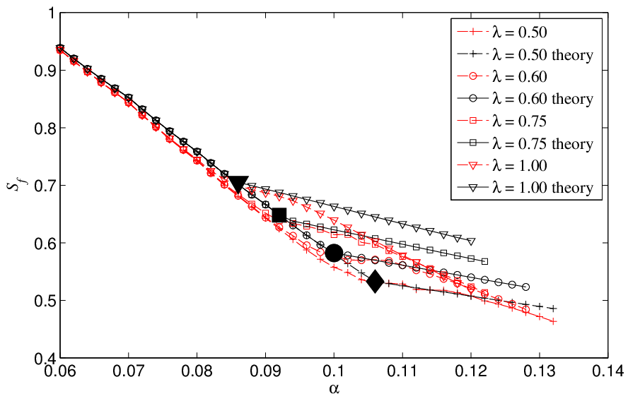
Before exploring the fraction of active nodes, we firstly investigate the complementary states consisting of failed and removed nodes. Fig. 3 presents the fractions of failed nodes and removed nodes with varied effective spreading rate in BA networks. When is small , the theoretical results are in good agreement with simulation results. While is large, there is a deviation between theoretical result and simulation result. The reason for this deviation is that nodes participates both bond percolation (epidemic spreading) and site percolation processes (cascading failure) are suppose to be the latter one in theoretical prediction. In simulation, a considerable amount of nodes are infected and become removed when is large. We can easily find that each of the curves of simulation and theoretical results has a turning point at abscissa . In Fig. 3, when is smaller than , is very close to zero, which means the epidemic dies out locally. While is larger than , is larger than zero, indicating the epidemic spreads out and infects a portion of the network. In Fig. 3, when is smaller than , decreases with increasing of . While is larger than , decreases more slowly, indicating the cascading failure slows down, and epidemic spreads out and infects a fraction of the network. This is an interesting phenomenon that even if the infection probability is very large, the epidemic still dies out when is smaller than . This is because, when is small, very few initial infected nodes can lead to severe cascading failure, which cuts off the spreading paths of the epidemic.

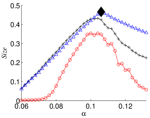
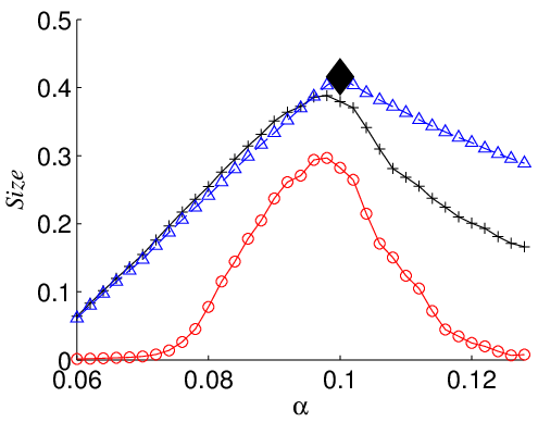
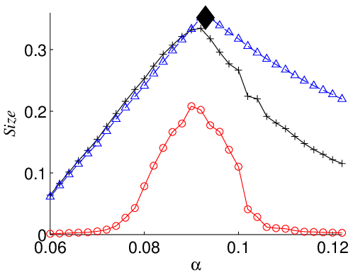

Then we explore the fraction of active nodes and the fraction of the giant component formed by them when the two dynamics of epidemic spreading and cascading failure are terminated, as shown in Fig. 4. Simulation and theoretical results of are both plotted. Because in a data communication network, the fraction of the largest connected sub-network formed by active nodes (the giant component of active nodes, ) is the important fraction to capture the robustness of the network with respect to structural damage and maintain the network functions [27]. Though the sizes of and are different, their humps meet the peaks at almost the same value which is very close to the critical value . This means that our theoretical method can be used to estimate the critical value as well as the optimal value of at which most active nodes are remained. It is worth noting that the fraction of active nodes is remarkably larger than that of standard SIR model (the size for remaining active nodes is very close to zero with large in standard SIR model), because in our model, the cascading failure blocks the spreading of the epidemic, as we have mentioned above.
5 Conclusion
In this paper, we explore a model based on the SIR epidemic spreading model and a local load sharing cascading failure model. With change of tolerance parameter , there exists a critical value that whether the epidemic with large is bocked by cascading failure. When , cascading failure cuts off abundant of paths and block the spreading of epidemic locally. While , epidemic spreads out and infects a fraction of the network. We propose a method for estimating which is applicable in uncorrelated networks. In simulation, we validate the effectiveness of this method in BA networks.
References
- [1] \NameZhou J., Liu Z. Li B. \REVIEWPhys. Lett. A3682007458.
- [2] \NamePastor-Satorras R. Vespignani A. \REVIEWPhys. Rev. Lett.8620013200.
- [3] \NameLiu Z. Hu B. \REVIEWEurophys. Lett.722005315.
- [4] \NameDel Genio C. I. House T. \REVIEWPhys. Rev. E882013040801.
- [5] \NameGuo D., Trajanovski S., van de Bovenkamp R., Wang H. Van Mieghem P. \REVIEWPhys. Rev. E882013042802.
- [6] \NameHernández D. G. Risau-Gusman S. \REVIEWPhys. Rev. E882013052801.
- [7] \NameMin B., Goh K.-I. Kim I.-M. \REVIEWEurophys. Lett.103201350002.
- [8] \NameSachtjen M., Carreras B. Lynch V. \REVIEWPhys. Rev. E6120004877.
- [9] \NameKinney R., Crucitti P., Albert R. Latora V. \REVIEWEur. Phys. J. B462005101.
- [10] \NameCohen R., Erez K., Ben-Avraham D. Havlin S. \REVIEWPhys. Rev. Lett.8520004626.
- [11] \NameHuang X., Vodenska I., Havlin S. Stanley H. E. \REVIEWSci. Rep.320131219.
- [12] \NameBorrvall C., Ebenman B. Jonsson T. \REVIEWEcol. Lett.32000131.
- [13] \NameCoffman Jr E., Ge Z., Misra V. Towsley D. \BookNetwork resilience: exploring cascading failures within bgp in proc. of \BookProc. 40th Annual Allerton Conference on Communications, Computing and Control, IL, USA, 2002 pp. 1–10.
- [14] \NameOuyang B., Jin X., Xia Y., Jiang L. Wu D. \REVIEWEurophys. Lett.106201428005.
- [15] \NameKermark M. Mckendrick A. \REVIEWProc. R. Soc. Lond. A1151927700.
- [16] \NameHeesterbeek J. \BookMathematical Epidemiology of Infectious Diseases: Model Building, Analysis and Interpretation Vol. 5 (John Wiley & Sons) 2000.
- [17] \NameDobson I., Carreras B. A. Newman D. E. \REVIEWProbab. Eng. Inf. Sci.19200515.
- [18] \NameSansavini G., Hajj M., Puri I. Zio E. \REVIEWEurophys. Lett.87200948004.
- [19] \NameMotter A. E. Lai Y.-C. \REVIEWPhys. Rev. E662002065102.
- [20] \NameWang B. Kim B. J. \REVIEWEurophys. Lett.78200748001.
- [21] \NameLi P., Wang B.-H., Sun H., Gao P. Zhou T. \REVIEWEur. Phys. J. B622008101.
- [22] \NameLehmann J. Bernasconi J. \REVIEWPhys. Rev. E812010031129.
- [23] \NameNewman M. E. J. \REVIEWPhys. Rev. E662002016128.
- [24] \NameKarrer B. Newman M. E. J. \REVIEWPhys. Rev. E822010016101.
- [25] \NameGleeson J. P. \REVIEWPhys. Rev. E772008046117.
- [26] \NameHackett A., Melnik S. Gleeson J. P. \REVIEWPhys. Rev. E832011056107.
- [27] \NameSerrano M. A., Krioukov D. Boguñá M. \REVIEWPhys. Rev. Lett.1062011048701.