Quantum spin models for the SU($n$)₁ Wess-Zumino-Witten model

Before constructing the wave functions, let us briefly review the SU($n$)₁ WZW model [67]. This rational CFT has $n$ primary fields, denoted by $\Lambda_{a}$, with $a=0,1,\ldots,n-1$, corresponding to particular SU($n$) irreducible representations. The primary field $\Lambda_{0}$ is an SU($n$) singlet, which is also the identity field with conformal weight $h(\Lambda_{0})=0$. The next primary field $\Lambda_{1}$ is the SU($n$) fundamental representation, corresponding to a single box when the SU($n$) irreducible representations are represented as the Young tableaux. In general, the primary field $\Lambda_{a}$ corresponds to a Young tableau with a single column and $a$ rows. Accordingly, $\Lambda_{a}$ consists of $\dim\Lambda_{a}=\binom{n}{a}$ components, and we write these components as $\Lambda_{a,\alpha}$, where $\alpha\in\{1,2,\ldots,\dim\Lambda_{a}\}$.

The central charge $c$, conformal weights $h(\Lambda_{a})$, and fusion rules of the SU($n$)₁ WZW model are given by [68]

As we shall discuss further below, the SU($n$)₁ WZW model has a free-field representation with $n-1$ free bosons. In this representation, the primary fields are conveniently realized using vertex operators.

To build lattice wave functions, we consider $N_{\text{T}}$ spins sitting at the fixed positions $z_{j}$ ($j=1,2,\ldots,N_{\text{T}}$) in the complex plane. Following Ref. [56], we define lattice wave functions

that are chiral correlators of primary fields. Here, $|0\rangle$ is the vacuum of the CFT and $|\alpha_{j}\rangle$ are the basis vectors of the internal state of spin number $j$. CFT states of the form (2) can be seen as a special type of matrix product states in which the finite-dimensional matrices have been replaced by infinite-dimensional conformal fields. They are therefore sometimes referred to as infinite-dimensional-matrix product states (IDMPS).

Regarding the wave function (2), there are several comments in order. First, choosing the primary field $\Lambda_{a_{j}}$ at site $j$ requires that the spin at this site also transforms under the SU($n$) irreducible representation corresponding to a Young tableau with one column and $a_{j}$ rows. Note that the SU($n$)₁ WZW model does not have primary fields corresponding to a Young tableaux with more than one column. Secondly, the fusion rules in (1) always have a unique fusion outcome, which ensures that the wave function (2) is a unique function. Lastly, to have a nonvanishing wave function, the $N_{\text{T}}$ primary fields in (2) must fuse into the identity $\Lambda_{0}$ (i.e. the SU($n$) singlet),

In this work, we shall focus on the case, where each of the spins belong either to the SU($n$) fundamental representation $\Lambda_{1}$ or to the SU($n$) conjugate representation $\Lambda_{n-1}$. We shall denote the sublattice of spins transforming under the fundamental (conjugate) representation by $A$ ($B$),

and we shall let $N$ ($\bar{N}$) denote the number of spins in $A$ ($B$) such that $N+\bar{N}=N_{\text{T}}$. The condition (3) then gives that $(N-\bar{N})/n$ must be an integer, and we shall assume this to be the case throughout. Note that the fundamental and conjugate representations are the same for $n=2$, so that there is only one state in this particular case. For $n\geq 3$, however, they are different.

Before we continue with the above case, let us note that other choices for the primary fields are possible. For instance, for even $n$, one could use the primary field $\Lambda_{n/2}$ (self-conjugate representation) to build the wave function, according to the fusion rule $\Lambda_{n/2}\otimes\Lambda_{n/2}\otimes\cdots\otimes\Lambda_{n/2}=\Lambda_{0}$ ($N_{\text{T}}$ even). For the SU(4) case, one has SU(4)${}_{1}\simeq$ SO(6)₁ and the SU(4) self-conjugate primary field $\Lambda_{2}$ becomes the vector representation of SO(6) with conformal weight $h(\Lambda_{2})=1/2$, which can be interpreted as a Majorana field and has been considered in Ref. [59]. Although we only consider states constructed from the fundamental and conjugate representations below, we note that the formalism we develop is general and that other cases can be treated in a similar way.

In the following, we shall find it convenient to use the notation

We can then write the wave functions that we are interested in as

where

Since we shall often refer to the wave function, for which all the primary fields belong to the fundamental representation, we shall give this wave function a particular name: $|\Psi_{\mathrm{F}}\rangle$. Explicit representations of $|\Psi_{\mathrm{F}}\rangle$ and $|\Psi\rangle$ will be discussed in Secs. III and V, respectively. In the next two subsections, we shall use their abstract forms to derive relevant null fields and their corresponding decoupling equations, which are our starting point for deriving parent Hamiltonians.

As a rational CFT, the SU($n$)₁ WZW model has null vectors in its Verma modules of the Kac-Moody algebra. According to Ref. [56], identifying proper null vectors and deriving decoupling equations for the chiral correlators are the key for constructing parent Hamiltonians of the wave functions. In this subsection, we derive the null vectors relevant for (7).

The SU($n$)₁ Kac-Moody algebra is defined by

where $J_{m}^{a}=\oint_{0}\frac{dz}{2\pi i}z^{m}J^{a}(z)$ is the $m$th mode of the Kac-Moody current $J^{a}(z)$ and $f_{abc}$ are the structure constants of the SU($n$) Lie algebra. Here and later on, we shall always assume that repeated indices are summed over. The operator product expansion (OPE) between the Kac-Moody currents and a primary field is [67]

where the matrices $t^{a}$ with elements $(t^{a})_{\alpha\beta}$ are the generators of SU($n$) in the representation of the primary field. Let us note here that the generators in the fundamental and conjugate representations are related though a complex conjugation and a multiplication by a minus sign, i.e.,

where $\tau^{a}$ are the generators in the fundamental representation (see Appendix A).

To the primary field $\varphi_{\alpha}(z)$, one associates a primary state $|\varphi_{\alpha}\rangle$ satisfying the following properties [67]:

and descendant states are obtained by multiplying $|\varphi_{\alpha}\rangle$ by any number of current operators $J_{n}^{a}$ with $n<0$. A null state is a state that is at the same time a descendant and a primary state. Since the wave function (7) only involves primary fields belonging to the fundamental or the conjugate representation, we shall here only need to deal with the two Verma modules formed by the corresponding primary states, as well as their descendants.

Let us first consider the primary field $\Lambda_{1,\alpha}(z)$ belonging to the fundamental representation. In Virasoro level $m=1$, we look for null vectors with the following form:

where $W_{q,a\alpha}$ can be interpreted as Clebsch-Gordan coefficients satisfying $\sum_{a\alpha}W_{q,a\alpha}^{\ast}W_{q^{\prime},a\alpha}=\delta_{qq^{\prime}}$. They come from the tensor product decomposition of the $(n^{2}-1)$-dimensional SU($n$) adjoint representation (carried by $J_{-1}^{a}$) and the fundamental representation (carried by $|\Lambda_{1,\alpha}\rangle$),

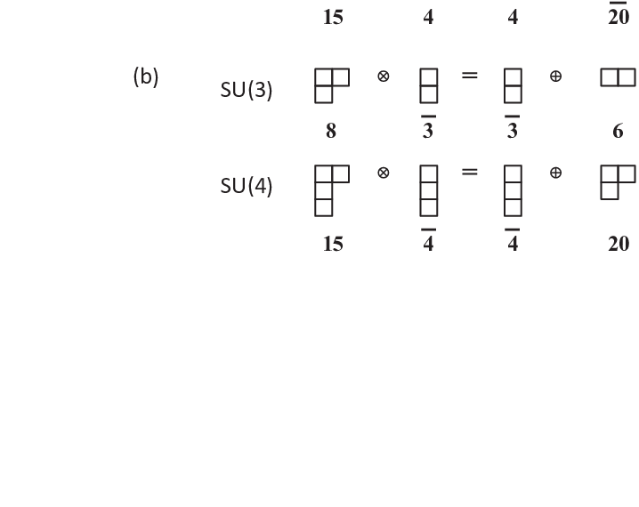
where the irreducible representations are denoted by their dimensions (they are not distinguished with their complex conjugate representations). Fig. 1(a) shows the tensor product decomposition (13) for $n=2,3,4$, using the Young tableaux. We have found that, for SU($n$)₁ WZW model with all $n$, null vectors indeed exist in Virasoro level $m=1$, and they belong to the SU($n$) representation with dimension $\frac{1}{2}n(n-1)(n+2)$ in (13). In practice, the Clebsch-Gordan coefficients $W_{q,a\alpha}$ in (12) can be determined by requiring the null vector condition $\langle\chi^{b^{\prime}}|\chi^{b}\rangle=0$.

For our purpose, we redefine the null vectors as [56]

where $(K_{\mathrm{F}})_{b\beta}^{a\alpha}$ is given by

$\mathbf{K}_{\mathrm{F}}$ can be viewed as a matrix with its entries being $(\mathbf{K}_{\mathrm{F}})_{a\alpha,b\beta}=(K_{\mathrm{F}})_{b\beta}^{a\alpha}$, and it is a projector (i.e. $\mathbf{K}_{\mathrm{F}}^{2}=\mathbf{K}_{\mathrm{F}}$) onto the SU($n$) irreducible representation with dimension $\frac{1}{2}n(n-1)(n+2)$. This also lead to an additional equation, $\sum_{a}t^{a}(K_{\mathrm{F}})_{b}^{a}=0$, where $(K_{\mathrm{F}})_{b}^{a}$ is a matrix with entries $[(K_{\mathrm{F}})_{b}^{a}]_{\alpha\beta}=(K_{\mathrm{F}})_{b\beta}^{a\alpha}$. These two equations are sufficient for determining the explicit form of $(K_{\mathrm{F}})_{b}^{a}$. For general $n$, we obtain

where $d_{abc}$ is a totally symmetric tensor (see Appendix A).

If we build the null vector at Virasoro level $m=1$ using the primary state $|\Lambda_{n-1,\alpha}\rangle$ in the conjugate representation, the representations appearing in (13) would be their complex conjugate representations. See Fig. 1(b) for this tensor product decomposition for $n=3$ and $4$. As a result, the Clebsch-Gordan coefficients in (12) for obtaining the null vectors would be their complex conjugate. Then, the corresponding null vectors can be written as

where $(K_{\mathrm{C}})_{b\beta}^{a\alpha}=(K^{\ast}_{\mathrm{F}})_{b\beta}^{a\alpha}$.

Utilizing (10), we can combine (14) and (17) into a single expression

where $K_{b\beta}^{a\alpha}$ are the matrix elements of

Here, $r=+1$ for the fundamental representation, $r=-1$ for the conjugate representation, and $t^{c}$ are the generators in the considered representation.

Following Ref. [56], a set of decoupling equations can be derived for the chiral correlator (7) using the null vectors (18). These decoupling equations provide operators annihilating the wave functions, which can be used to build parent Hamiltonians.

The null state (18) corresponds to the following null field:

By definition of the null field, substituting it into the wave function (7), one obtains a vanishing expression

After deforming the integral contour and using the OPE (9) between the Kac-Moody currents and primary fields, we arrive at

where $(K^{(i)})_{b}^{a}$ denotes the operator $K_{b}^{a}$ in (19) acting on spin number $i$ and $(t_{j}^{b})_{\alpha_{j}\alpha_{j}^{\prime}}$ denote the matrix elements of the operator $t^{b}$ acting on spin number $j$. (Note that the representation chosen for $t_{j}^{b}$ is the same as the representation of spin number $j$.) Thus, the resulting decoupling equation yields a set of operators

which annihilate the wave function $|\Psi\rangle$, i.e. $\mathcal{P}_{i}^{a}(z_{1},\ldots,z_{N})|\Psi\rangle=0$ $\forall i,a$. Together with the fact that $|\Psi\rangle$ is a global SU($n$) singlet, $T^{a}|\Psi\rangle=0$ with $T^{a}=\sum_{i}t_{i}^{a}$, we obtain

where $\mathcal{C}_{i}^{a}(z_{1},\ldots,z_{N})$ is given by

and $w_{ij}=(z_{i}+z_{j})/(z_{i}-z_{j})$. For SU(2), we have $d_{abc}=0$ and (25) recovers the result in Ref. [56]. Utilizing the formulas in Appendix A, we get

which is a convenient form for constructing parent Hamiltonians.

After working out the decoupling equations for (7) using an abstract form of the primary fields, we now turn to an explicit representation of these primary fields, using chiral vertex operators. This is possible, since SU($n$)₁ WZW model is equivalent to a free theory of $n-1$ massless bosons.

For our purpose, it is convenient to label the spin states in each site by their weights (eigenvalues of the Cartan generators). The state $|\alpha\rangle$, $\alpha\in\{1,2,\ldots,n\}$, in the fundamental representation is therefore characterized by $n-1$ quantum numbers, which we collect into the vector $\vec{m}_{\alpha}$ given explicitly by

In the conjugate representation, the state $|\alpha\rangle$, $\alpha\in\{1,2,\ldots,n\}$, is characterized by the quantum numbers $-\vec{m}_{\alpha}$. The SU(3) and SU(4) weight diagrams are shown in Fig. 2 as examples.

Using the weights, the primary field $\varphi_{\alpha}(z)$ can be expressed as

where $r=+1$ for the fundamental representation and $r=-1$ for the conjugate representation as above. The colons denote normal ordering and $\vec{\phi}(z)$ is a vector of $n-1$ independent fields of free, massless bosons. The factor $\kappa_{\alpha}$ is a Klein factor, commuting with the vertex operators and satisfying Majorana-like anticommutation relations

Note that $\kappa_{\alpha}$ is the same in the fundamental and in the conjugate representation. At this moment, the meaning of these Klein factors is not clear. In fact, their role is to ensure that the wave function (7) is an SU($n$) singlet. We will go back to this point when discussing the wave functions in Sec. III and Sec. V.

Let us note that the vertex operators in (28) have the anticipated conformal weights, since

Another quantity, which will be used in later sections, is $\vec{m}_{\alpha}\cdot\vec{m}_{\alpha^{\prime}}$ with $\alpha\neq\alpha^{\prime}$. It is easy to convince ourselves that this value does not depend on the states we choose. For $\alpha\neq\alpha^{\prime}$, we find

Altogether, we thus conclude

In order to compare the state (33) to known models in particular limits, we shall now express the state in a hardcore boson basis. In this picture, the coordinates $z_{j}$ are lattice sites that can be empty or occupied by at most one hardcore boson. A spin in the state $|n\rangle$ is interpreted as an empty site, and a spin in the state $|\alpha\rangle$, with $\alpha\in\{1,2,\ldots,n-1\}$, is interpreted as a site occupied by a hardcore boson with color $\alpha$.

Referring to (27), we observe that the $(n-1)$th component $m_{\alpha_{j},n-1}$ of the vector $\vec{m}_{\alpha_{j}}$ can be written as

where $p_{j}$ is one if $\alpha_{j}\in\{1,2,\ldots,n-1\}$ and zero if $\alpha_{j}=n$. In other words, we can use this component to distinguish between occupied sites and holes, and we shall use this observation to eliminate the coordinates of the unoccupied sites from the Jastrow factor in (33). The part of this factor that includes the contribution from $m_{\alpha_{j},n-1}$ can be written as

The second factor in the above expression can be simplified as [57, 60]

where

Let us next consider the part of the Jastrow factor that includes the contributions from $m_{\alpha_{j},l}$ with $l=1,2,\ldots,n-2$. Utilizing (27) and (32), we find

If $\alpha$ or $\alpha^{\prime}$ is equal to $n$, we instead get $\sum_{l=1}^{n-2}m_{\alpha,l}m_{\alpha^{\prime},l}=0$ as follows immediately from (27). The part of the Jastrow factor that includes the contributions for $m_{\alpha_{j},l}$ with $l=1,2,\ldots,n-2$ can therefore be written as

Combining (43) and (47), we get the expression

for the Jastrow factor.

We would like to also remove the hole coordinates from the sign factor $\chi$. Doing so gives rise to a sign factor that compensates the factor $\prod_{j}(-1)^{(j-1)p_{j}}$ in the wave function. The remaining sign factor is then $\mathrm{sgn}(x_{1}^{(1)},\ldots,x_{N/n}^{(1)},x_{1}^{(2)},\ldots,x_{N/n}^{(2)},\ldots,x_{1}^{(n-1)},\ldots,x_{N/n}^{(n-1)})$. We note, however, that this factor can be absorbed by rearranging the ordering in the Jastrow factor. Putting everything together, we thus conclude that the state (35) can also be written as

where the sum is over all possible distributions of the $(n-1)N/n$ colored bosons on the $N$ lattice sites with at most one boson per site, and

References

- [1] I. Affleck and J. B. Marston, Phys. Rev. B 37, 3774 (1988).
- [2] J. B. Marston and I. Affleck, Phys. Rev. B 39, 11538 (1989).
- [3] N. Read and S. Sachdev, Nucl. Phys. B 316, 609 (1989).
- [4] N. Read and S. Sachdev, Phys. Rev. B 42, 4568 (1990).
- [5] D. P. Arovas and A. Auerbach, Phys. Rev. B 38, 316 (1988).
- [6] A. Auerbach, Interacting electrons and quantum magnetism (Springer-Verlag New York, 1994).
- [7] Y. Li, M. Ma, D. Shi, and F. Zhang, Phys. Rev. Lett. 81, 3527 (1998).
- [8] Y. Yamashita, N. Shibata, and K. Ueda, Phys. Rev. B 58, 9114 (1998).
- [9] K. Kugel and D. Khomskii, Zh. Eksp. Teor. Fiz 64, 1429 (1973).
- [10] P. Azaria, A. O. Gogolin, P. Lecheminant, and A. A. Nersesyan, Phys. Rev. Lett. 83, 624 (1999).
- [11] R. Assaraf, P. Azaria, M. Caffarel, and P. Lecheminant, Phys. Rev. B 60, 2299 (1999).
- [12] M. van den Bossche, P. Azaria, P. Lecheminant, and F. Mila, Phys. Rev. Lett. 86, 4124 (2001).
- [13] G.-M. Zhang and S.-Q. Shen, Phys. Rev. Lett. 87, 157201 (2001).
- [14] T. A. Tóth, A. M. Läuchli, F. Mila, and K. Penc, Phys. Rev. Lett. 105, 265301 (2010).
- [15] P. Corboz, A. M. Läuchli, K. Penc, M. Troyer, and F. Mila, Phys. Rev. Lett. 107, 215301 (2011).
- [16] P. Corboz, K. Penc, F. Mila, and A. M. Läuchli, Phys. Rev. B 86, 041106 (2012a).
- [17] P. Corboz, M. Lajkó, A. M. Läuchli, K. Penc, and F. Mila, Phys. Rev. X 2, 041013 (2012b).
- [18] B. Bauer, P. Corboz, A. M. Läuchli, L. Messio, K. Penc, M. Troyer, and F. Mila, Phys. Rev. B 85, 125116 (2012).
- [19] P. Corboz, M. Lajkó, K. Penc, F. Mila, and A. M. Läuchli, Phys. Rev. B 87, 195113 (2013).
- [20] S. Taie, Y. Takasu, S. Sugawa, R. Yamazaki, T. Tsujimoto, R. Murakami, and Y. Takahashi, Phys. Rev. Lett. 105, 190401 (2010).
- [21] S. Taie, R. Yamazaki, S. Sugawa, and Y. Takahashi, Nat. Phys. 8, 825 (2012).
- [22] X. Zhang, M. Bishof, S. L. Bromley, C. V. Kraus, M. S. Safronova, P. Zoller, A. M. Rey, and J. Ye, arXiv:1403.2964 (2014).
- [23] F. Scazza, C. Hofrichter, M. Höfer, P. C. De Groot, I. Bloch, and S. Fölling, arXiv:1403.4761 (2014).
- [24] I. Bloch, J. Dalibard, and W. Zwerger, Rev. Mod. Phys. 80, 885 (2008).
- [25] M. A. Cazalilla and A. M. Rey, arXiv:1403.2792 (2014).
- [26] C. Wu, J. Hu, and S.-C. Zhang, Phys. Rev. Lett. 91, 186402 (2003).
- [27] C. Honerkamp and W. Hofstetter, Phys. Rev. Lett. 92, 170403 (2004).
- [28] M. Cazalilla, A. Ho, and M. Ueda, New J. Phys. 11, 103033 (2009).
- [29] A. Gorshkov, M. Hermele, V. Gurarie, C. Xu, P. Julienne, J. Ye, P. Zoller, E. Demler, M. Lukin, and A. Rey, Nat. Phys. 6, 289 (2010).
- [30] C. Xu, Phys. Rev. B 81, 144431 (2010).
- [31] S. R. Manmana, K. R. Hazzard, G. Chen, A. E. Feiguin, and A. M. Rey, Phys. Rev. A 84, 043601 (2011).
- [32] L. Messio and F. Mila, Phys. Rev. Lett. 109, 205306 (2012).
- [33] H. Nonne, M. Moliner, S. Capponi, P. Lecheminant, and K. Totsuka, EPL 102, 37008 (2013).
- [34] Z. Cai, H.-H. Hung, L. Wang, D. Zheng, and C. Wu, Phys. Rev. Lett. 110, 220401 (2013).
- [35] B. Frischmuth, F. Mila, and M. Troyer, Phys. Rev. Lett. 82, 835 (1999).
- [36] K. Harada, N. Kawashima, and M. Troyer, Phys. Rev. Lett. 90, 117203 (2003).
- [37] N. Kawashima and Y. Tanabe, Phys. Rev. Lett. 98, 057202 (2007).
- [38] R. K. Kaul, arXiv:1403.5678 (2014).
- [39] G. Uimin, JETP Letters 12, 225 (1970).
- [40] C. Lai, J. Math. Phys. 15, 1675 (1974).
- [41] B. Sutherland, Phys. Rev. B 12, 3795 (1975).
- [42] N. Kawakami, Phys. Rev. B 46, 3191(R) (1992).
- [43] Z. N. C. Ha and F. D. M. Haldane, Phys. Rev. B 46, 9359 (1992).
- [44] H. Kiwata and Y. Akutsu, J. Phys. Soc. Jpn. 61, 1441 (1992).
- [45] F. D. M. Haldane, Phys. Rev. Lett. 60, 635 (1988).
- [46] B. S. Shastry, Phys. Rev. Lett. 60, 639 (1988).
- [47] I. Affleck, D. Arovas, J. Marston, and D. Rabson, Nucl. Phys. B 366, 467 (1991).
- [48] S. Chen, C. Wu, S.-C. Zhang, and Y. Wang, Phys. Rev. B 72, 214428 (2005).
- [49] M. Greiter, S. Rachel, and D. Schuricht, Phys. Rev. B 75, 060401 (2007).
- [50] M. Greiter and S. Rachel, Phys. Rev. B 75, 184441 (2007).
- [51] D. P. Arovas, Phys. Rev. B 77, 104404 (2008).
- [52] R. Orús and H.-H. Tu, Phys. Rev. B 83, 201101 (2011).
- [53] I. Affleck, T. Kennedy, E. H. Lieb, and H. Tasaki, Phys. Rev. Lett. 59, 799 (1987).
- [54] I. Affleck, T. Kennedy, E. H. Lieb, and H. Tasaki, Commun. Math. Phys. 115, 477 (1988).
- [55] J. I. Cirac and G. Sierra, Phys. Rev. B 81, 104431 (2010).
- [56] A. E. B. Nielsen, J. I. Cirac, and G. Sierra, J. Stat. Mech. 2011, P11014 (2011).
- [57] A. E. B. Nielsen, J. I. Cirac, and G. Sierra, Phys. Rev. Lett. 108, 257206 (2012).
- [58] G. Moore and N. Read, Nucl. Phys. B 360, 362 (1991).
- [59] H.-H. Tu, Phys. Rev. B 87, 041103 (2013).
- [60] H.-H. Tu, A. E. B. Nielsen, J. I. Cirac, and G. Sierra, New J. Phys. 16, 033025 (2014).
- [61] A. E. B. Nielsen, G. Sierra, and J. I. Cirac, Nat. Commun. 4, 2864 (2013).
- [62] A. Kitaev and J. Preskill, Phys. Rev. Lett. 96, 110404 (2006).
- [63] M. Levin and X.-G. Wen, Phys. Rev. Lett. 96, 110405 (2006).
- [64] V. Kalmeyer and R. Laughlin, Phys. Rev. Lett. 59, 2095 (1987).
- [65] V. Kalmeyer and R. Laughlin, Phys. Rev. B 39, 11879 (1989).
- [66] X.-G. Wen, F. Wilczek, and A. Zee, Phys. Rev. B 39, 11413 (1989).
- [67] P. D. Francesco, P. Mathieu, and D. Sénéchal, Conformal Field Theory (Springer-Verlag New York, 1997).
- [68] P. Bouwknegt and K. Schoutens, Nucl. Phys. B 547, 501 (1999).
- [69] B. I. Halperin, Helv. Phys. Acta 56, 75 (1983).
- [70] H.-C. Jiang, Z. Wang, and L. Balents, Nat. Phys. 8, 902 (2012).
- [71] M. B. Hastings, I. González, A. B. Kallin, and R. G. Melko, Phys. Rev. Lett. 104, 157201 (2010).
- [72] F. D. M. Haldane, Z. N. C. Ha, J. C. Talstra, D. Bernard, and V. Pasquier, Phys. Rev. Lett. 69, 2021 (1992).
- [73] H. Blöte, J. L. Cardy, and M. Nightingale, Phys. Rev. Lett. 56, 742 (1986).
- [74] I. Affleck, Phys. Rev. Lett. 56, 746 (1986a).
- [75] K. Schoutens, Phys. Lett. B 331, 335 (1994).
- [76] P. Bouwknegt and K. Schoutens, Nucl. Phys. B 482, 345 (1996).
- [77] D. Schuricht and M. Greiter, EPL 71, 987 (2005).
- [78] D. Schuricht and M. Greiter, Phys. Rev. B 73, 235105 (2006).
- [79] I. Affleck, Nucl. Phys. B 265, 409 (1986b).
- [80] A. Läuchli, G. Schmid, and S. Trebst, Phys. Rev. B 74, 144426 (2006).
- [81] M. Führinger, S. Rachel, R. Thomale, M. Greiter, and P. Schmitteckert, Annalen der Physik 17, 922 (2008).
- [82] M. Aguado, M. Asorey, E. Ercolessi, F. Ortolani, and S. Pasini, Phys. Rev. B 79, 12408 (2009).
- [83] R. B. Laughlin, Ann. Phys. 191, 163 (1989).
- [84] D. F. Schroeter, Ann. Phys. 310, 155 (2004).
- [85] D. F. Schroeter, E. Kapit, R. Thomale, and M. Greiter, Phys. Rev. Lett. 99, 097202 (2007).
- [86] R. Thomale, E. Kapit, D. F. Schroeter, and M. Greiter, Phys. Rev. B 80, 104406 (2009).
- [87] E. Kapit and E. Mueller, Phys. Rev. Lett. 105, 215303 (2010).
- [88] M. Greiter, Mapping of Parent Hamiltonians: From Abelian and non-Abelian Quantum Hall States to Exact Models of Critical Spin Chains (Springer Tracts in Modern Physics vol 244) (Springer, Berlin, 2011).
- [89] M. Greiter, D. F. Schroeter, and R. Thomale, Phys. Rev. B 89, 165125 (2014).
- [90] B. Bauer, B. P. Keller, M. Dolfi, S. Trebst, and A. W. W. Ludwig, arXiv:1303.6963 (2013).
- [91] B. Bauer, L. Cincio, B. P. Keller, M. Dolfi, G. Vidal, S. Trebst, and A. W. W. Ludwig, arXiv:1401.3017 (2014).
- [92] A. E. B. Nielsen, G. Sierra, and J. I. Cirac, Phys. Rev. A 90, 013606 (2014).
- [93] M. Hermele, V. Gurarie, and A. M. Rey, Phys. Rev. Lett. 103, 135301 (2009).
- [94] M. Hermele and V. Gurarie, Phys. Rev. B 84, 174441 (2011).
- [95] C. Holzhey, F. Larsen, and F. Wilczek, Nucl. Phys. B 424, 443 (1994).
- [96] G. Vidal, J. I. Latorre, E. Rico, and A. Kitaev, Phys. Rev. Lett. 90, 227902 (2003).
- [97] P. Calabrese and J. Cardy, J. Stat. Mech. 2004, P06002 (2004).
- [98] H. Frahm and M. J. Martins, Nucl. Phys. B 862, 504 (2012).
- [99] R. Thomale, S. Rachel, P. Schmitteckert, and M. Greiter, Phys. Rev. B 85, 195149 (2012).
- [100] B. Paredes, Phys. Rev. B 85, 195150 (2012).
- [101] L. A. Takhtajan, Phys. Lett. A 87, 479 (1982).
- [102] H. Babujian, Phys. Lett. A 90, 479 (1982).
- [103] N. Y. Reshetikhin, Theor. Math. Phys. 63, 555 (1985).
- [104] H.-H. Tu and R. Orús, Phys. Rev. Lett. 107, 077204 (2011).
- [105] I. Affleck, Phys. Rev. Lett. 54, 966 (1985).
- [106] I. Affleck, J. Phys.: Condens. Matter 2, 405 (1990).
- [107] F. Michaud, F. Vernay, S. R. Manmana, and F. Mila, Phys. Rev. Lett. 108, 127202 (2012).
- [108] C. K. Majumdar and D. K. Ghosh, J. Math. Phys. 10, 1388 (1969).
- [109] R. Bondesan and T. Quella, arXiv:1405.2971, Nucl. Phys. B in press, DOI: 10.1016/j.nuclphysb.2014.07.002 (2014).
- [110] H. Georgi, Lie Algebras in Particle Physics (Perseus Books, Reading, MA, 1999).
- [111] A. Macfarlane, A. Sudbery, and P. Weisz, Commun. Math. Phys. 11, 77 (1968).