Imitation-based Social Spectrum Sharing
Abstract
Dynamic spectrum sharing is a promising technology for improving the spectrum utilization. In this paper, we study how secondary users can share the spectrum in a distributed fashion based on social imitations. The imitation-based mechanism leverages the social intelligence of the secondary user crowd and only requires a low computational power for each individual user. We introduce the information sharing graph to model the social information sharing relationship among the secondary users. We propose an imitative spectrum access mechanism on a general information sharing graph such that each secondary user first estimates its expected throughput based on local observations, and then imitates the channel selection of another neighboring user who achieves a higher throughput. We show that the imitative spectrum access mechanism converges to an imitation equilibrium, where no beneficial imitation can be further carried out on the time average. Numerical results show that the imitative spectrum access mechanism can achieve efficient spectrum utilization and meanwhile provide good fairness across secondary users.
I Introduction
Dynamic spectrum sharing is envisioned as a promising technique to alleviate the problem of spectrum under-utilization [2]. It enables unlicensed wireless users (secondary users) to opportunistically access the licensed channels owned by legacy spectrum holders (primary users), and thus can significantly improve the spectrum efficiency [3].
A key challenge of dynamic spectrum sharing is how to share the spectrum resources in an intelligent fashion. Most of existing works in dynamic spectrum sharing networks focus on exploring the individual intelligence of the secondary users. A common modeling approach is to consider that secondary users are fully rational, and model their interactions as noncooperative games (e.g., [4, 5, 6, 7, 8] and many others). Nie and Comniciu in [4] designed a self-enforcing distributed spectrum access mechanism based on potential games. Niyato and Hossain in [5, 9] studied a price-based spectrum access mechanism for competitive secondary users. Chen and Huang in [7] proposed a spatial spectrum access game framework for distributed spectrum sharing problem with spatial reuse. Li et al. in [6] proposed a game theoretic framework to achieve incentive compatible multi-band sharing among the secondary users.
When not knowing spectrum information such as channel availability, secondary users need to learn the network environment and adapt the spectrum access decisions accordingly. Han et al. in [10] used no-regret learning to solve this problem, assuming that the users’ channel selections are common information. When users’ channel selections are not observable, authors in [11, 12] designed multi-agent multi-armed bandit learning algorithms to minimize the expected performance loss of distributed spectrum access
The common assumption of all the above work is that secondary users act fully rationally based on individual intelligence. To have full rationality, a user typically needs to have a high computational power to collect and analyze the network information in order to predict other users’ behaviors. This is often not feasible due to the limitations of today’s wireless devices.
In this paper, we will explore the social intelligence of the secondary users based on social interactions. The motivation is to overcome the limited capability of today’s wireless devices by leveraging the wisdom of secondary user crowds. In fact, the emergence of social intelligence has been observed in many social interactions of animals [13] and has been utilized for engineering algorithm design. For example, Kennedy and Eberhart intended the particle swarm optimization algorithm by simulating social movement behaviors in a bird flock [14]. Pham et al. developed the bees algorithm by mimicing the food foraging behaviors of honey bees [15]. The understanding of human social phenomenon also sheds new light into the design of more efficient engineering systems such as wireless communication networks. For example, Wang and Yoneki in [16] exploited the social structure such as centrality and community to design efficient forwarding algorithms in opportunistic networks. The trust mechanism in human social activities has also been utilized to promote node cooperation in mobile ad hoc networks [17].
In this paper, we will design distributed spectrum access mechanism based on imitation, which is also a common phenomenon in many social animal and human interactions [18]. Imitation is simple (just follow a successful action of another user) and turns out to be an efficient strategy in many applications [19]. For example, Schlag in [20] used imitation to solve the multi-armed bandit problem. Lopes et al. in [21] designed an efficient imitation-based social learning mechanism for robots. Alos-Ferrer and Weidenholzer in [22] investigated the imitation strategy for the network coordination game. Imitation in wireless networks, however, has several fundamental differences from the previous approaches. For example, when too many wireless users imitate the same channel choice, then severe congestion in spectrum utilization will occur. Furthermore, different wireless users may experience different channel conditions due to the local environmental factors such as fading. Hence it is challenging to design an efficient mechanism based on imitation to deal with the user heterogeneity.
Recently, Iellamo et al. in [23] proposed an imitation-based spectrum access mechanism for spectrum sharing networks, by assuming that all the secondary users are homogeneous (i.e., they experience the same channel condition) and the true expected throughput on a channel is known by a secondary user once the user has chosen the channel. In this paper, we relax these restrictive assumptions and design an imitative spectrum access mechanism based on user’s local observations such as the realized data rates and transmission collisions. The key idea is that each user applies the maximum likelihood estimation to estimate its expected throughput, and imitates another neighboring user’s channel selection if neighbor’s estimated throughput is higher. Moreover, as imitation requires limited information sharing, we introduce the information sharing graph to model the social information sharing relationship among the secondary users. For example, in practical wireless systems it is often the case that a user can only receive message broadcasting from a subset of users that are close enough due to the geographical constraint. Moreover, we also generalize the proposed imitation based spectrum access mechanism to the case that secondary users are heterogeneous. The main results and contributions of this paper are as follows:
- •
Imitative Spectrum Access: We propose a novel imitation-based distributed spectrum access mechanism on a general information sharing graph. Each secondary user first estimates its expected throughput based on local observations, and then chooses to imitate a better neighbor. The imitation-based mechanism leverages the social intelligence of the secondary user crowd and only requires a low computational power for each individual user.
- •
Convergence to the Imitation Equilibrium: We show that the imitative spectrum access mechanism converges to the imitation equilibrium, wherein no imitation can be further carried out on the time average. When the information sharing graph is connected, we show that the imitation equilibrium corresponds to a fair channel allocation, such that all the users achieve the same throughput in the asymptotic case.
- •
Imitative Spectrum Access with User Heterogeneity: We further design an imitation-based spectrum access mechanism with user heterogeneity, where different users achieve different data rates on the same channel. Numerical results show that the proposed mechanism achieves up-to fairness improvement with at most performance loss, compared with the centralized optimal solution. This demonstrates that the proposed imitation-based mechanism can achieve efficient spectrum utilization and meanwhile provide good fairness across secondary users.
The rest of the paper is organized as follows. We introduce the system model in Section II. We then present the imitative spectrum access mechanism in Section III, and study the dynamics and convergence of the imitative spectrum access mechanism in Section IV. We proposed imitative spectrum access mechanism with user heterogeneity, and illustrate the performance of the proposed mechanisms through numerical results in Sections V and VI, respectively, Finally, we conclude the paper in Section VII.
II System Model
In this part, we first discuss the system model of distributed spectrum sharing, and then introduce the information sharing graph for the imitation mechanism.
II-A Spectrum Sharing System Model
We consider a spectrum sharing network with a set of independent and stochastically heterogeneous licensed channels. A set of secondary users try to opportunistically access these channels, when the channels are not occupied by primary (licensed) transmissions. For simplicity, we assume that all secondary users accessing the same channel will interfere with each other (i.e., the interference graph under the protocol interference model [24] is fully meshed). The case with the spatial reuse (i.e., the interference graph can be partially meshed) will be considered in a future work. The system model has a slotted transmission structure as in Figure 1 and is described as follows.
1) Channel State: the channel state for a channel during a time slot is
2) Channel State Changing: for a channel , we assume that the channel state is an i.i.d. Bernoulli random variable, with an idle probability and a busy probability . This model can be a good approximation of the reality if the time slots for secondary transmissions are sufficiently long or the primary transmissions are highly bursty [11]. The motivation of considering the i.i.d. channel state model is to focus our analysis on the spectrum contention due to secondary users’ dynamic channel selections. However, numerical results show that the proposed mechanism also works well in the Markovian channel environment where channel states have correlations between time slots. Please refer to Section VI-A2 for a detailed discussion.
3) Heterogeneous Channel Throughput: if a channel is idle, the achievable data rate by a secondary user in each time slot evolves according to an i.i.d. random process with a mean , due to the local environmental effects such as fading [25]. For example, we can compute the data rate according to the Shannon capacity as
| (1) |
where is the bandwidth of channel , is the fixed transmission power adopted by user according to the requirements such as the primary user protection, denotes the background noise power, and is the channel gain. In a Rayleigh fading channel environment, the channel gain is a random variable that follows the exponential distribution [25]. Here we first consider the homogeneous user case that all users achieve the same mean data rate on the same channel (but users can achieve different data rates on different channels). In Section V, we will further consider the heterogeneous user case that different users can achieve different mean data rates even on the same channel. This will allow users to have different transmission technologies, choose different coding/modulation schemes, and experience different channel conditions.
4) Time Slot Structure: each secondary user executes the following stages synchronously during each time slot:
- •
Channel Sensing: sense one of the channels based on the channel selection decision generated at the end of previous time slot (see below). Access the channel if it is idle.
- •
Channel Contention: use a backoff mechanism to resolve collisions when multiple secondary users access the same idle channel11 1 For ease of exposition, we adopt the backoff mechanism as an example. Our analysis can apply to many other medium access control (MAC) schemes such as TDMA.. The contention stage of a time slot is divided into mini-slots22 2 Note that in general the length of a mini-slot is much smaller than the length of spectrum sensing and access period in a time slot. For example, for IEEE 802.11af systems (also known as WhiteFi Networks), the length of a mini-slot is microseconds and the spectrum sensing duration is milliseconds [26]. (see Figure 1), and user executes the following two steps. First, count down according to a randomly and uniformly chosen integral backoff time (number of mini-slots) between and . Second, once the timer expires, transmit RTS/CTS messages if the channel is clear (i.e., no ongoing transmission). Note that if multiple users choose the same backoff value , a collision will occur with RTS/CTS transmissions and no users win the channel contention.
- •
Data Transmission: transmit data packets if the RTS/CTS message exchange is successful (i.e., the user wins the channel contention).
- •
Channel Selection: choose a channel to access in the next time slot according to the imitative spectrum access mechanism (introduced in Section III).
Suppose that users choose the same idle channel to access. Then the probability that a user (out of the users) successfully grabs the channel is
which is a decreasing function of the total contending users . Then the long-run expected throughput of a secondary user choosing a channel is given as
| (2) |

II-B Social Information Sharing Graph
In order to carry out imitations, we assume that there exists a common control channel for the information exchange among secondary users33 3 There are several approaches for establishing a common control channel in cognitive radio networks, e.g., sequence-based rendezvous [27], adaptive channel hopping [28] and user grouping [29]. Please refer to [30] for a comprehensive survey on the research of common control channel establishment in cognitive radio networks.. As an alternative, we can adopt the proximity-based communication approach [31], such that secondary users equipped with the radio interfaces such as near field communication (NFC)/bluetooth/WiFi Direct can communicate with each other directly for information exchange. Since information exchange typically would incur an overhead such as the extra energy consumption, it is important to design a proper incentive mechanism for stimulating collaborative information exchange among secondary users. One possible approach is to design mechanisms such that users receive exogenous incentives for cooperation. For example, a payment based incentive mechanism [32] compensates users’ contributions by rewarding them with virtual currency. In reputation based incentive mechanisms [33], users’ cooperative behaviors are monitored by some centralized authority or collectively by the whole user population, so that any user’s selfish behaviors would be detected and punished. In general, such an approach requires centralized infrastructures (e.g., secondary base-station/access point), which would incur a high system overhead and may not be feasible in our context of distributed spectrum sharing.
The centralized infrastructures are not available, motivated by the observation that the hand-held devices are typically carried by human beings, we can leverage the endogenous incentive which comes from the intrinsic social relationships among users to promote effective and trustworthy cooperation. For example, when a user is at home or work, typically family members, neighbors, colleagues, or friends are nearby. The user can then exploit the social trust from these neighboring users to achieve effective cooperation for information exchange. Indeed, with the explosive growth of online social networks such as Facebook and Twitter, more and more people are actively involved in online social interactions, and social connections among people are being extensively broadened. This has opened up a new avenue to integrate the social interactions for cooperative networking design.
Specifically, we introduce the social information sharing graph to model cooperative information exchange relationships due to the social ties among the secondary users. Here the vertex set is the same as the user set , and the edge set is given as where if and only if users and have social tie between each other, e.g., kinship, friendship, or colleague relationships. Furthermore, for a pair of users and who have a social edge between them on the social graph, we formalize the strength of social tie as , with a higher value of being a stronger social tie. Each secondary user can specify a cooperation threshold and is willing to share information with those users with whom he has a high enough social tie above the cooperation threshold . Moreover, to thwart the potential attacks of releasing false channel information by malicious users and enhance the security level of imitation based spectrum access, each secondary user can set a trust threshold and choose to trust the information from those users having a high enough social tie above the trust threshold . In the sequel, we denote the neighborhood of user for effective and trustworthy information sharing as . In terms of implementation, the social relationship identification procedure can be carried out prior to the imitative spectrum access. Specifically, two secondary users can locally initiate the “matching” process to detect the common social features between them. For example, two users can match their contact lists. If they have the phone numbers of each other or many of their phone numbers are the same, then it is very likely that they know each other. As another example, two device users can match their home and working addresses and identify whether they are neighbors or colleagues. To preserve the privacy of the secondary users, the private set intersection and homomorphic encryption techniques proposed in [34, 35] can be adopted to design a privacy-preserving social relationship identification mechanism.
We should emphasize that when it is difficult to leverage the social trust among some secondary users and the centralized infrastructures are not available, similar to the file sharing in the P2P systems [36], we can adopt the Tit-for-Tat mechanism for information sharing. Specifically, based on the principle of reciprocity, a secondary user will always share information with its partner as long as its partner (i.e., another user) also shares information with it. If the partner refuses to share information, the user will punish its partner by not sharing information either. As a result, the partner would suffer and learn to share information with the user again. Notice that since the imitative spectrum access mechanism can work on a generic social information sharing graph, we can also use a hybrid approach of several different schemes mentioned above for establishing the information sharing relationships among the secondary users.
Since our analysis is from secondary users’ perspective, we will use terms “secondary user” and “user” interchangeably in the following sections.
III Imitative Spectrum Access Mechanism
We now apply the idea of imitation to design an efficient distributed spectrum access mechanism, which utilizes user’s local estimation of its expected throughput. Each user randomly chooses a neighboring user in the information sharing graph, and follows the neighbor’s channel selection if the neighbor’s throughout is better than its.
III-A Expected Throughput Estimation
In order to imitate a successful action, a user needs to compare its and other users’ performances (throughputs). In practice, many wireless devices only have a limited view of the network environment due to hardware constraints. To incorporate the effect of incomplete network information, we first introduce the maximum likelihood estimation (MLE) approach to estimate user’s expected throughput based on its local observations. We choose MLE mainly due to the efficiency and the ease of implementation of this method [37]. To achieve accurate local estimation based on local observations, a user needs to gather a large number of observation samples. This motivates us to divide the spectrum access time into a sequence of decision periods indexed by , where each decision period consists of time slots (see Figure 2 for an illustration). During a single decision period, a user accesses the same channel in all time slots. Thus the total number of users accessing each channel does not change within a decision period, which allows users to learn the environment.
According to (2), a user’s expected throughput during decision period depends on the probability of grabbing the channel on that period, the channel idle probability , and the mean data rate .

III-A1 MLE of Channel Grabbing Probability
At the beginning of each time slot of a decision period , we assume that a user chooses to sense the same channel . If the channel is idle, the user will contend to grab the channel according to the backoff mechanism in Section II. At the end of each time slot , a user observes , , and . Here denotes the state of the chosen channel (i.e., whether occupied by the primary traffic), indicates whether the user has successfully grabbed the channel, i.e.,
and is the received data rate on the chosen channel by user at time slot . Note that if (i.e., the channel is occupied by the primary traffic), we set and to be . At the end of each decision period , each user will have a set of local observations .
When channel is idle (i.e., no primary traffic), consider users contend for the channel according to the backoff mechanism in Section II. Then a particular user out of these users grabs the channel with the probability . Since there are a total of rounds of channel contentions in the period and each round is independent, the total number of successful channel captures by user follows the Binomial distribution. User then computes the likelihood of , i.e., the probability of the realized observations given the parameter as
| (3) |
Then MLE of can be computed by maximizing the log-likelihood function , i.e., . By the first order condition, we obtain the optimal solution as which is the sample averaging estimation. When the length of decision period is large, by the central limit theorem, we know that where denotes the normal distribution.
III-A2 MLE of Channel Idle Probability
We next apply the MLE to estimate the channel idle probability Since the channel state is i.i.d over different time slots and different decision periods, we can improve the estimation by averaging not only over multiple time slots but also over multiple periods.
Similarly with MLE of , we first compute one-period MLE of as . When the length of decision period is large, we have that follows the normal distribution with the mean , i.e.,
We then average the estimation over multiple decision periods. When a user finishes accessing a channel for a total periods, it updates the estimation of the channel idle probability as , where is the estimation of based on the information of all decision periods, and is the one-period estimation. By doing so, we have which reduces the variance of one-period MLE by a factor of .
III-A3 MLE of Average Data Rate
Since the received data rate is also i.i.d over different time slots and different decision periods, similarly with the MLE of the channel idle probability , we can obtain the one-period MLE of mean data rate as , and the averaged MLE estimation over periods as
By the MLE, we can obtain the estimation of , , and as , and , respectively, and then estimate the true expected throughput as Since , , and follow independent normal distributions with the mean , , and , respectively, we thus have i.e., the estimation of expected throughput is unbiased. In the following analysis, we hence assume that
| (4) |
where is the random estimation noise with the probability density function satisfying
| (5) | |||
| (6) |
III-B Imitative Spectrum Access
We now propose the imitative spectrum access mechanism in Algorithm 1. The key motivation is that, by leveraging the social intelligence of the secondary user crowd, the imitation based mechanism only requires a low computational power for each individual user. More specifically, we let users imitate the actions of those neighboring users that achieve a higher throughput (i.e., Lines to in Algorithm 1). This mechanism only relies on local throughput comparisons and is easy to implement in practice. Each user at each period first collects the local observations (i.e., Lines to in Algorithm 1) and estimates its expected throughput with the MLE method as introduced in Section III-A (i.e., Line in Algorithm 1). Then user carries out the imitation by randomly sampling the estimated throughput of another user who shares information with him (i.e., Line in Algorithm 1). Such a random sampling can be achieved in different ways. For example, user can randomly generate a user ID from the set and broadcast a throughput enquiry packet including the enquired user ID . Then user will send back an acknowledgement packet including the estimation of its own expected throughput.
Intuitively, the benefits of adopting the imitation based channel selection are two-fold. On one hand, since each user has incomplete network information, by enquiring another user’s throughput information, each user would have a better view of channel environment. If a channel offers a higher data rate, more users trend to exploit the channel due to the nature of imitation. On the other hand, if too many users are utilizing the same channel, a user can improve its data rate through congestion mitigation by imitating users on another channel with less contending users. In the following Section IV, we show that the proposed imitation-based mechanism can drive a balance between good channel exploitation and congestion mitigation, and achieve a fair spectrum sharing solution.
We shall emphasize that, in the imitative spectrum access mechanism, we require that each user can (randomly) select only one user for the throughput enquiry, in order to promote diversity in users’ channel selections for further congestion mitigation and reduce the system overhead for information exchange. We also evaluate the imitative spectrum access schemes, such that each user can select multiple users for throughput enquiry and imitate the channel selection of the best user among these inquired users (please refer to Section for more details in the separate appendix file). We observe that the performance of the imitative spectrum access decreases as the number of users for throughput enquiry increases. This is because when each user imitates the best channel selection from multiple users, as the number of enquired users increases, the probability that more users will simultaneously select the same good channel to access in next time slot will increase. This would reduce the diversity of users’ channel selections (i.e., increases channel congestion) and hence lead to performance degradation in spectrum sharing, compared with the case of randomly enquiring only one user. Moreover, enquiring multiple users in the same time period will incur a higher system overhead for information exchange.
IV Convergence of Imitative Spectrum Access
We then investigate the convergence of imitative spectrum access. Since users’ imitations reply on the information exchange, the structure of the information sharing graph hence plays an important role on the convergence of the mechanism. To better understand the structure property, we will introduce an equivalent and yet more compact cluster-based graphical representation of the information sharing graph.
IV-A Cluster-based Graphical Representation of Information Sharing Graph
We now introduce the cluster-based presentation. The cluster concept here is similar with the community structure in social networks analysis [38, 22]. Intuitively, a cluster here can be viewed as a set of users who have similar information sharing structure. Formally, we define that
Definition 1 (Cluster).
A set of users form a cluster if they can share information with each other and they can also share information with the same set of users that are out of the cluster.
Taking the information sharing graph on the left hand-side in Figure 3 as an example, we see that users to form a cluster. However, users to do not form a cluster, since user shares information with user while user does not. Furthermore, we can regard a single user as a special case of cluster. In this case, a general information sharing graph can be represented compactly as a cluster-based graph. Let be the set of clusters, and denote the information sharing relationship between two clusters and . The variable if cluster communicates with cluster (i.e., the users in cluster share information with the users in cluster ) and otherwise. Then we denote the cluster-based graph as . Here vertex set is the cluster set, and edge set . We also denote the set of clusters that communicates with cluster as . Since the users in cluster and the users in cluster can share information with each other, we also define that .
As illustrated in Figure 3, an information sharing graph can be represented as different cluster-based graphs (e.g., graphs (c) and (e) in Figure 3). In general fact, we can first consider the original information sharing graph as a primitive cluster-based graph by regarding each single user as a cluster (e.g., graph (a) in Figure 3). We then further carry out the clustering (e.g., graph (d) in Figure 3) and obtain the cluster-based graph (e). We next merge clusters and of this cluster-based graph into one cluster and then obtain the most compact cluster-based graph (c) in this example. We summarize the algorithm for constructing the cluster-based graph in Algorithm 2. Note that for the practical implementation, the knowledge of cluster-based graphs is not required. The use of clutter-based graph here is to facilitate the analysis of the convergence of imitative spectrum access mechanism. The convergence properties of the imitative spectrum access mechanism are determined by the original information exchange graph, and are the same for all these cluster-based graphs since they preserve the structural property of the original information exchange graph (i.e., two users share information in the cluster-based graph if and only if they share information in the original graph).
Next we explore the property of the cluster-based representation. We denote the cluster that a user belongs to as and the set of users in cluster as . According to the definition of cluster, we can see that if users and share information with each other, then they either belong to the same cluster or two different clusters that communicate with each other. Thus we have that
Lemma 1.
The set of users that share information with user is the same as the set of users in user ’s cluster and the clusters that communicate with user ’s cluster, i.e., .
Furthermore, the cluster-based representation also preserves the connectivity of the information sharing graph (i.e., it is possible to find a path from any node to any other node).
Lemma 2.
The information sharing graph is connected if and only if the corresponding cluster-based graph is also connected.


IV-B Dynamics of Imitative Spectrum Access
Based on the cluster-based graphical representation of information sharing graph, we next study the evolution dynamics of the imitative spectrum access mechanism. Suppose that the underlying information sharing graph can be represented by clusters, and the number of users in each cluster is with . For the ease of exposition, we will focus the case that the number of users in each cluster is large. Numerical results show that the observations also hold for the case that the number of users in a cluster is small (see Sections VI for details).
With a large cluster user population, it is convenient to use the population state to describe the dynamics of spectrum access. We then denote the population state of all users as and the population state of cluster as . Here denotes the fraction of users in cluster choosing channel to access at period , and we have .
In the imitative spectrum access mechanism, each user relies on its local estimated expected throughput to decide whether to imitate other user’s channel selection. Due to the random estimation noise , the evolution of the population state is stochastic and difficult to analyze directly. However, when the population of cluster users is large, due to the law of large number, such stochastic process can be well approximated by its mean deterministic trajectory [39]. Here is the deterministic population state of all the users, and is the deterministic population state of cluster . Consider a user in cluster chooses channel , and let denote the probability that this user in the deterministic population state will choose channel in next period. According to [39], we have
Lemma 3.
There exists a scalar such that, for any bound , decision period , and any large enough cluster size , the maximum difference between the stochastic and deterministic population states over all periods is upper-bounded by with an arbitrarily large probability, i.e.,
| (7) |
given that .
The proof is similar with Lemma in [39] and hence is omitted here. As illustrated in Figure 4, Lemma 3 indicates that the trajectory of the stochastic population state is within a small neighborhood of the trajectory of the deterministic population state when the user population is large enough. Moreover, since the MLE is unbiased, the deterministic population state is also the mean field dynamics of stochastic population state [39]. If the deterministic dynamics converge to an equilibrium, the stochastic dynamics must also converge to the same equilibrium on the time average [39].
We now study the evolution dynamics of the deterministic population state . Let denote the expected throughput of a user that chooses channel with a total of contending users in the population state . Recall that in the imitative spectrum access mechanism, each user will randomly choose another user that shares information with it, and imitate that user’s channel selection if that user’s estimated throughput is higher. Suppose that the user is in cluster choosing channel . According to Lemma 1, the set of users that share information with user are in set of clusters . Thus, we can obtain the probability that this user will imitate another user on channel in next period as
| (8) |
Here denotes the probability that a user choosing channel in cluster will be selected for imitation. From (4), we have
| (9) |
where are the random estimation noises with the probability density function . Let , and we can obtain the probability density function of random variable as
| (10) |
We further denote the cumulative distribution function as , i.e., . Then from (8) and (9), we have for any ,
| (11) |
and
| (12) |
Based on (11) and (12), we obtain the evolution dynamics of the deterministic population state as (the proof is given in Section VIII-A in the separate appendix file)
Theorem 1.
For the imitative spectrum access mechanism, the evolution dynamics of deterministic population state are given as
| (13) |
where the derivative is with respect to time .
IV-C Convergence of Imitative Spectrum Access
We now study the convergence of the imitative spectrum access mechanism. Let denote the equilibrium of the imitative spectrum access, and denote the channel chosen by user in the equilibrium . We first introduce the definition of imitation equilibrium.
Definition 2 (Imitation Equilibrium).
A population state is an imitation equilibrium if and only if for each user ,
| (14) |
where denotes the set of channels are chosen by users that share information with user in the equilibrium .
The intuition of Definition 2 is that no imitation can be carried out to improve any user’s data rate in the equilibrium. For the imitative spectrum access mechanism, we show that
Theorem 2.
For the imitative spectrum access mechanism, the evolution dynamics of deterministic population state asymptotically converge to an imitation equilibrium such that
| (15) |
The proof is given in Section VIII-B in the separate appendix file. According to Lemma 3, we know that the stochastic imitative spectrum access dynamics will be attracted into a small neighborhood around the imitation equilibrium . Moreover, since the imitation equilibrium is also the mean field equilibrium of stochastic dynamics , the stochastic dynamics hence converge to the imitation equilibrium on the time average. That is, the fraction of users adopting a certain channel selection will converge to a fixed vale on the time average. However, a user would keep switching its channel during the process. This is because that when many other users also utilize the same channel, the user would imitate to select another channel with less contending users to mitigate congestion. The mechanism hence can drive a balance between good channel exploitation and congestion mitigation.
According to the definition of , we see from Theorem 2 that two users will achieve the same expected throughput if they share information with each other (i.e., they are neighbors in the information sharing graph). Moreover, when the information sharing graph is connected, we can show that all the users achieve the same throughput at the imitation equilibrium.
Corollary 1.
When the information sharing graph is connected, all the users following the imitative spectrum access mechanism achieve the same expected throughput, i.e.,
The proof is given in Section VIII-C in the separate appendix file. Furthermore, we can show in Corollary 2 that the convergent imitation equilibrium is the most fair channel allocation in terms of the widely-used Jain’s fairness index ) [40]. Notice that the fair channel allocation is due to the nature of imitation. If the channel allocation is unfair, there must exist some secondary users that achieve a higher throughput than others. In this case, other users with a lower throughput will imitate the channel selection of those users until the performance of all users are equal (i.e., fair spectrum sharing).
Corollary 2.
When the information sharing graph is connected, the Jain’s fairness index is maximized at the imitation equilibrium.
The proof is given in Section VIII-D in the separate appendix file. We next discuss the efficiency of the imitation equilibrium. Similar to the definition of price of anarchy (PoA) in game theory, we will quantify the efficiency ratio of imitation equilibrium over the centralized optimal solution and define the price of imitation (PoI) as
Since it is difficult to analytically characterize the PoI for the general case, we focus on the case that all the channels are homogenous, i.e., and for any . Let be the number of channels being utilized at the imitation equilibrium , i.e., . We can show the following result.
Theorem 3.
When the information sharing graph is connected and all the channels are homogenous, the PoI of imitative spectrum access mechanism is at least
The proof is given in Section VIII-E in the separate appendix file. We also evaluate the performance of imitative spectrum access mechanism for the general case in Section VI. Numerical results demonstrate that the mechanism is efficient, with at most performance loss, compared with the centralized optimal solution.
V Imitative Spectrum Access With User Heterogeneity
For the ease of exposition, we have considered the case that users are homogeneous, i.e., different users achieve the same data rate on the same channel. We now consider the general heterogeneous case where different users may achieve different data rates on the same channel.
Let be the realized data rate of user on an idle channel at a time slot , and be the mean data rate of user on the idle channel , i.e., . In this case, the expected throughput of user is given as . For imitative spectrum access mechanism in Algorithm 1, each user carries out the channel imitation by comparing its throughput with the throughput of another user. However, such throughput comparison may not be feasible when users are heterogeneous, since a user may achieve a low throughput on a channel that offers a high throughput for another user.
To address this issue, we propose a new imitative spectrum access mechanism with user heterogeneity in Algorithm 3. More specifically, when a user on a channel randomly selects another neighboring user on another channel , user informs user about the estimated channel grabbing probability instead of the estimated expected throughput. Then user will compute the estimated expected throughput on channel as
| (16) |
If , then user will imitate the channel selection of user .
To implement the mechanism above, each user must have the information of its own estimated channel idle probability and data rate of the unchosen channel . Hence we add an initial channel estimation stage in the imitative spectrum access mechanism in Algorithm 3. In this stage, each user initially estimates the channel idle probability and data rate by accessing all the channels in a randomized round-robin manner. This ensures that all users do not choose the same channel at the same period. Let (equals to the empty set initially) be set of channels probed by user and . At beginning of each decision period, user randomly chooses a channel (i.e., a channel that has not been accessed before) to access. At end of the period, user can estimate the channel idle probability and data rate according to the MLE method introduced in Section III-A.
Numerical results show that the proposed imitative spectrum access mechanism with user heterogeneity can still converge to an imitation equilibrium satisfying the definition in (2), i.e., no user can further improve its expected throughput by imitating another user. Numerical results show that the imitative spectrum access mechanism with user heterogeneity achieves up-to fairness improvement with at most performance loss, compared with the centralized optimal solution. This demonstrates that the proposed imitation-based mechanism can achieve efficient spectrum utilization and meanwhile provide good fairness across secondary users.
Initial Channel Estimation Stage
Imitative Spectrum Access Stage
VI Simulation Results
In this section, we evaluate the proposed imitative spectrum access mechanisms by simulations. We consider a spectrum sharing network consisting Rayleigh fading channels. The data rate on an idle channel of user is computed according to the Shannon capacity, i.e., where is the bandwidth of channel , is the power adopted by user , is the noise power, and is the channel gain (a realization of a random variable that follows the exponential distribution with the mean ). By setting different mean channel gain , we can have different mean data rates . In the following simulations, we set MHz, dBm, and mW. We set the number of time slots in each decision period as . We will consider both cases with homogeneous and heterogenous users.
VI-A Imitative Spectrum Access with Homogeneous Users
VI-A1 I.i.d. Channel Environment


We first implement the imitative spectrum access mechanism with homogeneous users (i.e., Algorithm 1) and the number of backoff mini-slots . For each user , the mean channel data rates Mbps, respectively. The channel states are i.i.d. Bernoulli random variable with the mean idle probabilities , respectively.
We consider that the information sharing graphs are represented by different cluster-based graphs as shown in Figure 5. In Graph (a), clusters and do not communicate directly and they are connected to cluster . In Graph (b), all three clusters are isolated. We show the time average user’s throughput in Figure 6. We see that all the users achieve the same average throughput on Graph (a). This verifies the theoretic result that when information sharing graph is connected (i.e., the corresponding cluster-based graph is connected), all the users achieve the same average throughput in the imitation equilibrium. When information sharing graph is not connected (e.g., Graph (b)), we see that users in different clusters may achieve different throughputs. However, all the users in the same cluster have the same average throughput. This is also an imitation equilibrium given the constraint of their information sharing. Moreover, we see that all the channels will be utilized in the imitation equilibria on both Graphs (a)and (b). A channel of a higher data rate will be utilized by a larger fraction of users.
VI-A2 Markovian Channel Environment
For the interests of obtaining closed form solutions and deriving engineering insights, we have considered the i.i.d. channel model so far. We now evaluate the proposed mechanism in the Markovian channel environment. We denote the channel state probability vector of channel at a time slot as which follows a two-states Markov chain as , with the transition matrix In this case, we can obtain the stationary distribution that the channel is idle with a probability of . The study in [41] shows that the statistical properties of spectrum usage from empirical measurement data can be accurately captured and reproduced by properly setting the transition matrix. In this experiment, we choose different and for different channels such that the idle probabilities are the same as before. We consider that users are randomly scattered across a square area of a side-length of m with the information sharing graph as shown in Figure 7. As mentioned in Section IV-A, this information sharing graph can also be regarded as a cluster-based graph by considering a single user as a cluster.
The results are shown in the upper part of Figure 8. We observe that the imitative spectrum access mechanism still achieves the imitation equilibrium in the Markovian channel environment. The average throughput that each user achieves is the same as that in i.i.d. channel environment on the connected graph (a) in Figures 6. This is because that our proposed Maximum Likelihood Estimation of the channel idle probability follows the sample average approach. By the law of large numbers, when the observation samples are sufficient, such a sample average approach can achieve an accurate estimation of the average statistics of the channel availability, even if the channel state is not an i.i.d. process.


VI-B Imitative Spectrum Access with Heterogeneous Users
We then implement the imitation spectrum access mechanism with heterogeneous users (i.e., Algorithm 3) on the same information sharing graph in Figure 7. The mean data rates of randomly chosen users out of these users are homogeneous with the same data rates as before (i.e., Mbps). For the remaining users, we set that the users’ data rates are heterogenous with the mean data rate of user on channel as where is a random value drawn from the uniform distribution over . The results are shown in the bottom part of Figure 8. We see that the mechanism converges to the equilibrium wherein homogeneous users achieve the same expected throughput and heterogenous users may achieve different expected throughputs. Moreover, we observe that the mechanism converges to a stable user distribution on channels. This implies that no user can further improve its expected throughput by imitating another user. That is, the equilibrium is an imitation equilibrium satisfying the definition in (14).
VI-C The Impact of Information Exchange Delay
Next we evaluate the impact of the information exchange delay on the imitative spectrum access mechanism. Similar as in Section VI-A2, we consider that the spectrum sharing network consists of Rayleigh fading channels with the mean data rates Mbps, respectively. The primary activities are Markovian with the channel idle probabilities , respectively. The number of secondary users with the social information sharing graph given in Figure 7. We implement the imitative spectrum access mechanism, such that in each decision period a secondary user receives the delayed throughput information from other users and carries out the imitation based on the delayed information. Figure 9 shows the results with the information exchange delay , and decision periods, respectively. We observe that the proposed imitative spectrum access mechanism is quite robust to the information exchange delay. When the delay is not very large (e.g., periods), the mechanism can still converge to the same imitation equilibrium as the case without delay. When the delay is too large (e.g., periods), the mechanism fails to converge to the imitation equilibrium, since the throughput information is completely out-dated.

VI-D Performance Comparison
We now compare the proposed imitative spectrum access mechanism with the imitation-based spectrum access mechanism in [23]. Notice that the mechanism in [23] requires the global network information including the channel characteristics and other users’ channel selections to compute user’s throughput. When users are homogenous (i.e., different users achieve the same data rate on the same channel), both mechanisms can converge to the imitation equilibrium and hence achieve the same performance.
We now focus on performance comparisons for the more general and practical case that users are heterogenous. As the benchmark, we also implement the centralized optimal solution that maximizes the system-wide throughput (i.e., ) and the decentralized spectrum access solution by Q-learning mechanism proposed in [42]. Similarly to the setting in Section VI-B, we consider randomly scattered users, respectively. The mean data rate of user on channel is , where is a random value drawn from the uniform distribution over . For each fixed user number , we average over runs.
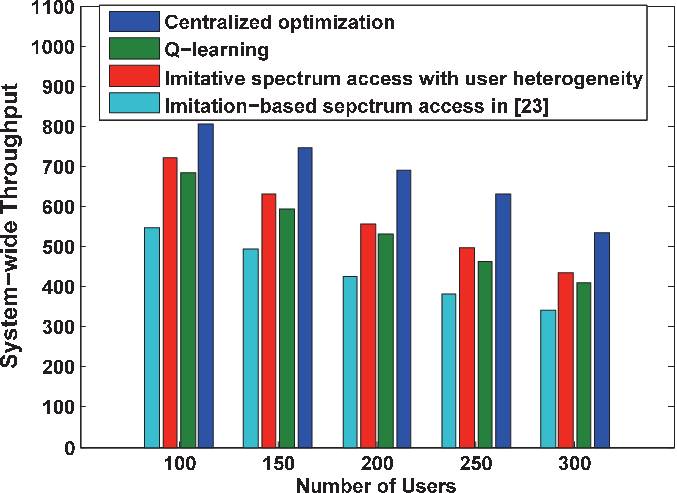
We first show the system-wide throughput achieved by different mechanisms in Figure 10. We see that the system-wide throughput of all the solutions decreases as the number of users increases. As the user population increases, the contention among users becomes more severe, which leads to more spectrum access collisions. We observe that the proposed imitative spectrum access mechanism with user heterogeneity achieves up-to performance improvement over the imitation-based spectrum access mechanism in [23]. This is because that the mechanism in [23] carries out imitation based on other user’s throughput information directly, which ignores the fact that users are heterogeneous. While our mechanism takes user heterogeneity into account and carries out imitation based on the channel contention level. Compared with Q-learning mechanism, the imitative spectrum access mechanism can achieve better performance, with a performance gain of around . Moreover, the performance loss of the imitative spectrum access mechanism with respect to the centralized optimal solution is at most in all cases. This demonstrates the efficiency of the imitative spectrum access mechanism with user heterogeneity.
We then compare the fairness achieved by different mechanisms in Figure 11. We adopt the widely-used Jain’s fairness index [40] to measure the fairness. A larger index represents a more fair channel allocation, with the best case . Figure 11 shows that the centralized optimal solution is poor in terms of fairness (with the highest index value ). This reason is that the centralized optimal solution would allocate the best channels to a small fraction of users only (to avoid congestion) and most users will share those channels of low data rates. Our imitative spectrum access is much more fair and achieves up to and fairness improvement over the centralized optimization and Q-learning, respectively. This demonstrates that the proposed imitation-based mechanism can provide good fairness across users.
VII Conclusion
In this paper, we design a distributed spectrum access mechanism with incomplete network information based on social imitations. We show that the imitative spectrum access mechanism can converge to an imitation equilibrium on different information sharing graphs. When the information sharing graph is connected and users are homogeneous, the imitation equilibrium corresponds to a fair channel allocation such that all the users achieve the same throughput. We also extend the imitative spectrum access mechanism to the case that users are heterogeneous. Numerical results demonstrate that the proposed imitation-based mechanism can achieve efficient spectrum utilization and meanwhile provide good fairness across secondary users.
To get useful initial insights of imitation for the distributed spectrum access mechanism design with incomplete network information, we have assumed that all the users interfere with each other in the spectrum sharing network. We plan to further extend our study to the case with spatial reuse. How to design an efficient imitation based spectrum access mechanism where each user only interferes with a subset of users in the spectrum sharing network is very challenging.
References
- [1] X. Chen and J. Huang, “Imitative spectrum access,” in 10th International Symposium on Modeling and Optimization in Mobile, Ad Hoc and Wireless Networks (WiOpt), 2012.
- [2] FCC, “Report of the spectrum efficiency group,” in Spectrum Policy Task Force, 2002.
- [3] C. Partridge, “Realizing the future of wireless data communications,” Communications of the ACM, vol. 54, no. 9, pp. 62–68, 2011.
- [4] N. Nie and Comniciu, “Adaptive channel allocation spectrum etiquette for cognitive radio networks,” in IEEE DySPAN, 2005.
- [5] D. Niyato and E. Hossain, “Competitive spectrum sharing in cognitive radio networks: a dynamic game approach,” IEEE Transactions on Wireless Communications, vol. 7, pp. 2651–2660, 2008.
- [6] D. Li, Y. Xu, J. Liu, X. Wang, and Z. Han, “A market game for dynamic multi-band sharing in cognitive radio networks,” in IEEE International Conference on Communications (ICC). IEEE, 2010, pp. 1–5.
- [7] X. Chen and J. Huang, “Spatial spectrum access game: Nash equilibria and distributed learning,” in Proceedings of the thirteenth ACM international symposium on Mobile Ad Hoc Networking and Computing. ACM, 2012, pp. 205–214.
- [8] D. Niyato and E. Hossain, “Dynamics of network selection in heterogeneous wireless networks: an evolutionary game approach,” IEEE Transactions on Vehicular Technology, vol. 58, no. 4, pp. 2008–2017, 2009.
- [9] D. Niyato, E. Hossain, and Z. Han, “Dynamics of multiple-seller and multiple-buyer spectrum trading in cognitive radio networks: A game-theoretic modeling approach,” IEEE Transactions on Mobile Computing, vol. 8, no. 8, pp. 1009–1022, 2009.
- [10] Z. Han, C. Pandana, and K. J. R. Liu, “Distributive opportunistic spectrum access for cognitive radio using correlated equilibrium and no-regret learning,” in IEEE Wireless Communications and Networking Conference (WCNC), 2007.
- [11] A. Anandkumar, N. Michael, and A. Tang, “Opportunistic spectrum access with multiple users: learning under competition,” in The IEEE International Conference on Computer Communications (Infocom), 2010.
- [12] K. Liu and Q. Zhao, “Decentralized multi-armed bandit with multiple distributed players,” in Information Theory and Applications Workshop (ITA), 2010.
- [13] D. Sumpter, Collective animal behavior. Princeton Univ Pr, 2010.
- [14] J. Kennedy and R. Eberhart, “Particle swarm optimization,” in IEEE International Conference on Neural Networks, vol. 4, 1995, pp. 1942–1948.
- [15] D. Pham, A. Ghanbarzadeh, E. Koc, S. Otri, S. Rahim, and M. Zaidi, “The bees algorithm–a novel tool for complex optimisation problems,” in IPROMS conference, 2006, pp. 454–461.
- [16] N. Wang and E. Yoneki, “Impact of social structure on forwarding algorithms in opportunistic networks,” in International Conference on Selected Topics in Mobile and Wireless Networking (iCOST), 2011.
- [17] J. Cho, A. Swami, and I. Chen, “A survey on trust management for mobile ad hoc networks,” IEEE Communications Surveys & Tutorials, no. 99, pp. 1–22, 2010.
- [18] W. Wyrwicka, Imitation in human and animal behavior. Transaction Pub, 1996.
- [19] C. SCHLAG, “Imitation and learning,” The Handbook of Rational and Social Choice, 2009.
- [20] K. Schlag, “Why imitate, and if so, how? a boundedly rational approach to multi-armed bandits,” Journal of Economic Theory, vol. 78, pp. 130–156, 1998.
- [21] M. Lopes, F. S. Melo, and L. Montesano, “Affordance-based imitation learning in robots,” in IEEE/RSJ International Conference on Intelligent Robots and Systems, 2007.
- [22] C. Alós-Ferrer and S. Weidenholzer, “Contagion and efficiency,” Journal of Economic Theory, vol. 143, no. 1, pp. 251–274, 2008.
- [23] S. Iellamo, L. Chen, and M. Coupechoux, “Let cognitive radios imitate: Imitation-based spectrum access for cognitive radio networks,” arXiv:1101.6016, Tech. Rep., 2011.
- [24] P. Gupta and P. Kumar, “The capacity of wireless networks,” IEEE Transactions on Information Theory, vol. 46, no. 2, pp. 388–404, 2000.
- [25] T. Rappaport, Wireless communications: principles and practice. Prentice Hall PTR New Jersey, 1996, vol. 2.
- [26] A. B. Flores, R. E. Guerra, E. W. Knightly, P. Ecclesine, and S. Pandey, “Ieee 802.11 af: A standard for tv white space spectrum sharing,” IEEE Communications Magazine, vol. 51, no. 10, pp. 92 – 100, 2013.
- [27] L. A. DaSilva and I. Guerreiro, “Sequence-based rendezvous for dynamic spectrum access,” in 3rd IEEE Symposium on New Frontiers in Dynamic Spectrum Access Networks. IEEE, 2008, pp. 1–7.
- [28] K. Bian, J.-M. Park, and R. Chen, “Control channel establishment in cognitive radio networks using channel hopping,” IEEE Journal on Selected Areas in Communications, vol. 29, no. 4, pp. 689–703, 2011.
- [29] L. Lazos, S. Liu, and M. Krunz, “Spectrum opportunity-based control channel assignment in cognitive radio networks,” in 6th Annual IEEE Communications Society Conference on Sensor, Mesh and Ad Hoc Communications and Networks. IEEE, 2009, pp. 1–9.
- [30] B. Lo, “A survey of common control channel design in cognitive radio networks,” Physical Communication, 2011.
- [31] R. J. Drost, R. D. Hopkins, R. Ho, and I. E. Sutherland, “Proximity communication,” IEEE Journal of Solid-State Circuits, vol. 39, no. 9, pp. 1529–1535, 2004.
- [32] L. Anderegg and S. Eidenbenz, “Ad hoc-VCG: a truthful and cost-efficient routing protocol for mobile ad hoc networks with selfish agents,” in Proceedings of the 9th annual international conference on Mobile computing and networking. ACM, 2003, pp. 245–259.
- [33] P. Michiardi and R. Molva, “Core: a collaborative reputation mechanism to enforce node cooperation in mobile ad hoc networks,” in Advanced Communications and Multimedia Security. Springer, 2002, pp. 107–121.
- [34] R. Zhang, Y. Zhang, J. Sun, and G. Yan, “Fine-grained private matching for proximity-based mobile social networking,” in IEEE INFOCOM. IEEE, 2012, pp. 1969–1977.
- [35] M. Von Arb, M. Bader, M. Kuhn, and R. Wattenhofer, “Veneta: Serverless friend-of-friend detection in mobile social networking,” in IEEE International Conference on Wireless and Mobile Computing, Networking and Communications. IEEE, 2008, pp. 184–189.
- [36] B. Cohen, “Incentives build robustness in bittorrent,” in Workshop on Economics of Peer-to-Peer systems, vol. 6, 2003, pp. 68–72.
- [37] T. Ferguson, A Course in Large Sample Theory. Chapman & Hall, 1996.
- [38] J. Scott, “Social network analysis,” Sociology, vol. 22, no. 1, p. 109, 1988.
- [39] M. Benam and J. Weibull, “Deterministic approximation of stochastic evolution in games,” Econometrica, vol. 71, pp. 873–903, 2003.
- [40] R. Jain, D. Chiu, and W. Hawe, “A quantitative measure of fairness and discrimination for resource allocation in shared computer systems,” DEC Research Report TR-301, 1984.
- [41] M. Lopez-Benitez and F. Casadevall, “Empirical time-dimension model of spectrum use based on a discrete-time markov chain with deterministic and stochastic duty cycle models,” Vehicular Technology, IEEE Transactions on, vol. 60, no. 6, pp. 2519–2533, 2011.
- [42] H. Li, “Multi-agent Q-learning for competitive spectrum access in cognitive radio systems,” in Fifth IEEE Workshop on Networking Technologies for Software Defined Radio (SDR) Networks., 2010.
- [43] K. S. Narendra and A. Annaswamy, Stable Adaptive Systems. Prentice Hall, 1989.
VIII Proofs
VIII-A Proof of Theorem 1
VIII-B Proof of Theorem 2
To proceed, we first define the following function
| (17) |
We then consider the variation of along the evolution trajectory of deterministic population state , i.e., differentiating with respective to time ,
| (18) |
Since is a probability density function satisfying , for all and , it follows from (10) that , for all and , for all . Hence the cumulated probability function is strictly increasing for any , and further , for all and , for all . This implies that if ,
| (19) |
and if ,
| (20) |
From (18), (19) and (20), we have . Hence is non-increasing along the trajectory of the evolution dynamics. According to the Lasalle’s principle [43], the evolution dynamics of deterministic population state must asymptotically converge to a limit point such that i.e.,
| (21) |
According to Lemma 1, the set of users that share information with user is the same as the set of users in user ’s cluster and the clusters that communicate with user ’s cluster, i.e., . Thus we must have where . This corresponds to the imitative equilibrium. ∎
VIII-C Proof of Corollary 1
Since the information sharing graph is connected, for any two different users and , there must exists a path satisfying that . According to Theorem 2, we have Since , it implies that ∎
VIII-D Proof of Corollary 2
According to Cauchy-Schwarz inequality, we know that and if and only if , for any . It then follows that Jain’s fairness index is maximized at the imitation equilibrium, since the condition holds according to Corollary 1. ∎
VIII-E Proof of Theorem 3
First of all, according to Corollary 1, we know that all the users at the imitation equilibrium achieve the same throughput. Since all the channels are homogenous, the number of users on each of utilized channels is the same, . It then follows that the system-wide throughput at the imitation equilibrium is On the other hand, for the centralized optimal solution, since for any , we know that . Thus, we can conclude that the PoI is at least . ∎