A quantum algorithm for additive approximation of Ising partition functions
Abstract
We investigate quantum computational complexity of calculating partition functions of Ising models. We construct a quantum algorithm for an additive approximation of Ising partition functions on square lattices. To this end, we utilize the overlap mapping developed by Van den Nest, Dür, and Briegel [Phys. Rev. Lett. 98, 117207 (2007)] and its interpretation through measurement-based quantum computation (MBQC). We specify an algorithmic domain, on which the proposed algorithm works, and an approximation scale, which determines the accuracy of the approximation. We show that the proposed algorithm does a nontrivial task, which would be intractable on any classical computer, by showing the problem solvable by the proposed quantum algorithm are BQP-complete. In the construction of the BQP-complete problem coupling strengths and magnetic fields take complex values. However, the Ising models that are of central interest in statistical physics and computer science consist of real coupling strengths and magnetic fields. Thus we extend the algorithmic domain of the proposed algorithm to such a real physical parameter region and calculate the approximation scale explicitly. We found that the overlap mapping and its MBQC interpretation improves the approximation scale exponentially compared to a straightforward constant depth quantum algorithm. On the other hand, the proposed quantum algorithm also provides us a partial evidence that there exist no efficient classical algorithm for a multiplicative approximation of the Ising partition functions even on the square lattice. This result supports that the proposed quantum algorithm does a nontrivial task also in the physical parameter region.
I Introduction
Classical spin models have been widely studied in statistical physics for a long time as simplified pictures of magnetic materials. The Ising model is the simplest model consisting of two discrete spin variables, up and down, but exhibits a rich structure enough to be applied not only for magnetic materials, but also lattice gases [1], binary alloys, neural systems [2] and economic models [3]. One of the main goal is to calculate a partition function, which tells us statistical properties of a system in thermodynamic equilibrium, such as free energy, magnetization, specific heat, and so on. Many techniques have been developed to calculate the Ising partition functions in both exact and approximated manners so far. Only restricted type of Ising models, such as Ising models on two-dimensional planer lattices without magnetic fields, are exactly solvable [4, 5]. In general, exact calculation of Ising partition functions belongs to #P-hard problems, which are highly intractable in classical computer [6]. Furthermore, even an efficient (multiplicative) approximation of antiferromagnetic Ising partition functions on general lattices does not exist unless RP = NP [7, 8], which is highly implausible to occur [9, 10]. It is a natural question how quantum computer is useful in this context [12, 11].
Recently quantum information theory sheds new light on computational complexity of Ising partition functions. Bravyi and Raussendorf argued classical simulatability of measurement-based quantum computation (MBQC) [13] on the planer surface codes by mapping it into an Ising partition function on a planer lattice [14]. Van den Nest, Dür, and Briegel established a correspondence between the quantum-stabilizer formalism and classical spin models [15]. In this mapping, a partition function of a classical spin model is expressed as an overlap between a stabilizer state and a product state. This overlap mapping allows us to apply powerful results obtained in the context of quantum information theory to statistical physics [15, 16]. Although a transfer matrix approach and a state overlap have already appeared in an earlier work [12], the overlap mapping makes the problem much more tractable, allowing us to interpret the overlap as MBQC and associated quantum circuits. For example, Van den Nest, Dür, and Briegel showed that the Ising model on a square lattice is complete in the sense that a partition function of any classical spin model on an arbitrary graph can be expressed as a certain instance of it [17, 18]. Furthermore, classical simulatability of MBQC on certain stabilizer states provides us an efficient classical algorithm to calculate the corresponding partition functions [15, 19]. Based on this mapping, De las Cuevas et al. proposed a quantum algorithm to approximate partition functions of classical spin models, such as Ising, Potts, vertex, and gauge models, in a complex parameter regime [20]. Furthermore, they showed that additive approximations of certain classical spin models are BQP-complete. (BQP stands for bounded-error quantum polynomial time computation and is a class of decision problems that can be efficiently solvable by a quantum computer.) This means that all problems that are solvable by quantum computer can be mapped into these problems. The consequences of this result are twofold. Firstly, at least for these types of classical spin models, we can utilize a quantum computer to estimate their partition functions efficiently. Secondary, BQP-completeness implies that there is less possibility to do this task on a classical computer. (If it is possible, we can simulate a quantum computer by a classical computer, which is highly implausible.)
Besides, quantum computational complexity of not only Ising partition functions but also link invariants such as Jones and Tutte polynomials has been argued also in the circuit models [22, 23, 21, 24, 25], and their additive approximations have been shown to be BQP-complete. Recently a sampling problem related to Ising partition functions has been shown to be intractable on any classical computer, while it can be done by using commutable quantum circuits [26], so-called instantaneous quantum polynomial time computation (IQP), which seems to be much weaker than universal quantum computation [27]. These results provide a clew to understand not only complexity of calculating classical spin models but also problems that are solvable by a quantum computer and the origin of quantum a speedup.
In this paper, we further investigate complexity of calculating Ising partition functions based on the overlap mapping [15] and its interpretation through MBQC. We specifically consider a quantum algorithm that approximates Ising partition functions on square lattices, where each instance of the problem is encoded into the coupling strengths and magnetic fields. In this sense, the present work is complimentary to those works done in Ref. [28, 20], in which instances of the problem is encoded into topology of the graphs taking the coupling strengths and magnetic fields homogeneously. Furthermore, we specify a domain, on which the proposed quantum algorithm works, and an approximation scale, which determines the accuracy of the additive approximation. We also provide a proof that the problem solved by the proposed quantum algorithm is BQP-hard. This indicates that the proposed quantum algorithm does a nontrivial task, which would be intractable on any classical computer.
We also establish a way to approximate general Ising partition functions including real coupling strengths and magnetic fields, which are especially of interest in statistical physics. In such a physical parameter region, the gate operations done by MBQC are not unitary anymore, and linear operators in general. Thus we construct a quantum algorithm that approximates such linear operators following the methods taken in Refs. [23, 21]. This allows us to clarify the approximation scale for general coupling strengths and magnetic fields.
We should note that a related work has been done by Iblisdir et al. recently [25]. In their work, certain types of quantum circuits are mapped into the Ising partition functions on square lattices. Specifically, they utilize a transfer matrix approach to map quantum circuits into the Ising partition functions. (A similar approach has been also taken in an earlier work [12].) The construction of the quantum algorithm in this work can be regarded as a measurement-based version of these works, which would be simpler for people who are familiar with MBQC. They have also considered approximation of the Ising partition functions with real coupling strengths and magnetic fields, while a rather different approach, analytic continuation, was taken (see also a related work [11]). Instead of analytic continuation, we here straightforwardly simulate linear operators by using unitary circuits. Since the proposed quantum algorithm provides the approximation scale explicitly for all parameter region, the proposed quantum algorithm allows us to compare the performances. Furthermore, the quantum circuits that approximate the physical Ising partition functions are also provide explicitly, which would be helpful to understand performance of the proposed quantum algorithm in the physical parameter region.
Unfortunately, it is still unknown whether or not the proposed quantum algorithm does a nontrivial task in the physical parameter region. However, we also provides a partial evidence that a multiplicative approximation of the Ising partition functions in the physical parameter region cannot be attained by any classical computer unless the polynomial hierarchy collapses at the third level. This result strongly supports that the proposed quantum algorithm actually does a nontrivial task even in the physical parameter region. We believe these quantum algorithms in the real parameter regime and their approximation scales provide an essential clue to understand potential of quantum computation in solving problems that takes an important role in combinatorial optimization problems.
The rest of the paper is organized as follows. In Sec. II, we review the correspondence between the quantum stabilizer formalism and the Ising partition functions with fixing the notations. In Sec. III, we propose a quantum algorithm that approximates the Ising partition functions on square lattices. We also show that the proposed quantum algorithm solves a BQP-complete problem and hence does a nontrivial task, which would be intractable on any classical computer. In Sec. IV, we extend the domain of the proposed quantum algorithm to general coupling strengths and magnetic fields, which include real parameters. We calculate the approximation scale of the quantum algorithm in this domain and argue the performance of the proposed quantum algorithm in the physical parameter region. Section V is devoted to conclusions and discussions.
II Quantum formulation of Ising model
In this section, we briefly review the correspondence between the quantum-stabilizer formalism and Ising partition functions with fixing the notations. We consider a classical Ising model defined on a graph with and being sets of vertices and edges, respectively. The Ising model consists of classical two-state spin variables defined on each vertex of the graph . Two spins and connected by an edge interact with each other by a coupling strength . Furthermore, each spin is subjected to a local magnetic field . The Hamiltonian of the system is given by
| (1) |
where indicates a spin configuration. The partition function is defined by
| (2) |
where the summation is taken over all spin configurations, and is the inverse temperature, , with and being the Boltzmann constant and the temperature, respectively.

We express the partition function as an inner product between a product state and a stabilizer state [17]. We first define the stabilizer state, which is described as a graph state associated with another graph . The graph , which we call a decorated graph, is defined by adding a vertex on each edge of the graph as shown in Fig. 1. The decorated graph has vertices and edges. The set of vertices is defined by , where corresponds to the set of vertices added on the edges. The set of edges is defined by . Assigning a qubit on each vertex in , we define a -qubit stabilizer state:
| (3) |
where , is taken over all configurations of , and denotes the addition modulo 2. The binary variable is related with the Ising spin later. The qubits belonging to and are referred to as vertex and edge qubits, respectively. We can easily confirm is a stabilizer state, since it can be obtained as
| (4) |
where indicates the controlled- gate between qubit (control) and (target), and denotes the set of vertices adjacent to vertex on the decorated graph . Let be the graph state associated with the graph [29]. Using the equality , is related with the graph state as follows:
| (5) |
where is the Hadamard gate acting on edge qubit on .
Next we define a product state with which the stabilizer state is taken an inner product:
| (6) |
where the single-qubit states are defined as
| (7) | ||||
| (8) |
for all vertices and .
Now we relate the Ising partition function with the inner product between the product state and the graph state as follows:
| (9) |
where the approximation scale is defined by
| (10) |
Eq. (9) can be understood as follows. The stabilizer state (or the graph state ) has information of the geometry of the Ising interactions. More precisely, each vertex qubit has a superposition of spin up and down states, and each edge qubit encodes the information whether the two spins interacting with are parallel or antiparallel. Depending on the state of the vertex and edge qubits, weights and are assigned by the product state through the inner product. Then, the superposition of all spin states is reduced to the summation over all spin configuration, which recovers the partition functions in the l.h.s. of Eq. (9).
Next we translate the overlap Eq. (9) into quantum computation, which is one of the most important task to establish a bridge between quantum computation and Ising partition functions. The states and can be expressed by using unitary gates and acting on the computational basis state respectively:
| (11) |
where we defined unitary gates
| (12) | ||||
| (13) |
Then, the product state can be rewritten as
| (14) |
where is defined as a tensor product of single-qubit gates. On the other hand, by virtue of the properties of the graph state [30], there exists a -qubit unitary gate such that
| (15) |
Specifically, if the degree of the graph is finite as considered here, is a constant depth Clifford circuit consisting of Hadamard gates and controlled- gates. Then Eq. (9) is rewritten as
| (16) |
The quantum circuit consisting of only quantum gates can be efficiently implemented on a quantum computer. The matrix element of can be estimated by using the Hadamard test (see e.g. [21, 22, 23]) as shown in Fig. 2.

More precisely, we can obtain an approximation of within the following additive error:
| (17) |
Accordingly the partition function of Eq. (9) can be efficiently approximated with an additive error .
The approximation scale of the above quantum algorithm is far from optimal, since we utilized only constant depth quantum circuits. By using the idea of MBQC, we can compress the number of qubits employed utilizing non-constant depth quantum circuits. This allows us to improve the approximation scale as follows. The overlap is regarded as an MBQC implemented by the sequence of projections on the resource state . If the projection satisfies a certain condition such that the MBQC interpretation works appropriately, we can rewrite the overlap as teleportation-based -qubit quantum computation
| (18) |
where is a non-constant depth quantum circuit. Note that the number of qubits in the r.h.s. are reduced compared to that in the l.h.s. By using this identity, Eq. (9) can be rewritten as
| (19) |
where an approximation scale is defined as . By using the hadamard test to evaluate the r.h.s., the partition function is approximated with an additive error . Note that the approximation scale is exponentially improved from . On the other hand, computation time is increased only polynomially. Thus we can still obtain an exponential improvement of the accuracy of the approximation taking into account the computation time. A detail of embedding the Ising models in MBQC tells us the improved approximation scale and the algorithmic domain as seen below.
III A quantum algorithm for Ising partition functions
In this section, we propose a quantum algorithm to approximate the partition function of the Ising model by establishing a mapping between a class of Ising models and MBQC.

We consider an Ising model on an square lattice with [see Fig. 3 (a)]. We define vertical and horizontal coupling strengths, and , for the vertical and horizontal edges , respectively. The Hamiltonian is given by
| (20) |
where and are the sets of vertical and horizontal edges, respectively. Specifically, we consider the following problem:
Problem 1
(Approximation of Ising partition functions) Consider an Ising model on an square lattice, where . The magnetic fields and the vertical coupling strengths are arbitrary imaginary numbers and the horizontal coupling strengths are given by , where is a real number and is an integer. The problem is defined as an approximation of the partition function of the given Ising Hamiltonian with an additive error , where the approximation scale is given by .
In the following subsections, we will show two theorems:
Theorem 1 (Quantum algorithm)
There exists an efficient quantum algorithm that solves Problem 1.
Theorem 2 (BQP-hardness)
Problem 1 is BQP-hard.
By combining these results, we will conclude the following theorem:
Theorem 3 (BQP-completeness)
Consider Problem 1 and is promised to be either or . Then the problem to decide whether or not is BQP-complete.
III.1 Construction of quantum algorithm
(proof of Theorem 1)
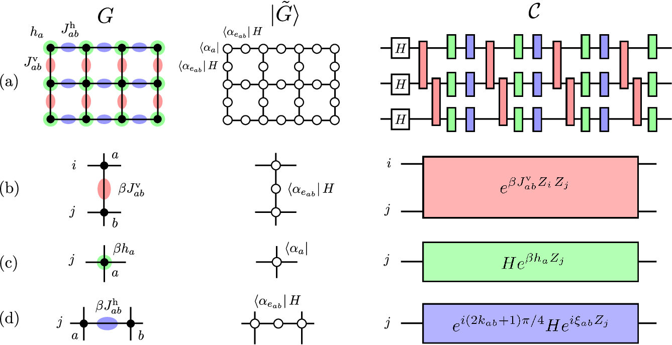
In this subsection, we prove Theorem 1. We first construct a quantum algorithm which solves Problem 1. To this end, we interpret horizontal edges of the graph as wires of an -qubit quantum circuit. According to the coupling strengths and magnetic fields, quantum gates are assigned on the wires from the left to the right as follow [see Fig. 4 (a)]:
- (i)
are assigned as initial gates.
- (ii)
According to the vertical coupling strength , A two-qubit gate is assigned on the corresponding th and th wires. Since is an imaginary number, is a two-qubit unitary gate. Specifically, if , an identity gate is assigned.
- (iii)
According to the magnetic field , a single-qubit gate is assigned on the corresponding th wire. Since is an imaginary number, is a single qubit unitary gate.
- (iv)
According to the horizontal coupling strength , we assign a single-qubit gate on the corresponding th wire. Here is an angle that satisfies . [Recall that .]
- (v)
After the above procedure, we obtain a quantum circuit
| (21) |
where the multiplication is performed over all vertices of the decorated graph from the left to right columns. In the same column, the multiplications for vertical edge qubits are taken at first, and then those for vertex qubits are taken secondarily.
Next we will show that the quantum circuit is related to the partition function as
| (22) |
We interpret the projection by as a sequence of measurements in MBQC, whose resource state is given by the graph state . The measurements are assumed to be performed from the left to the right. (In the projection , the measurement outcomes are always determined, and there is no feedforward in the present MBQC interpretation. Thus we chose a convenient measurement order, from the left to the right, without loss of generality.) As shown below, the projection by induces a sequence of unitary gates in a measurement-based way, which corresponds to the -qubit quantum circuit constructed.
The projection on the vertical edge qubit can be written as
| (23) |
Here indicates a graph state associated with the decorated graph, where vertex and adjacent edges are deleted. This tells us that the projection on the vertical edge qubit on can be replaced by the two-qubit gate on the corresponding wires as shown in Fig. 4 (b).
The projection on the vertex qubit is regarded as quantum teleportation, which propagates quantum information from the left to the right with a single-qubit unitary gate. The standard argument for MBQC [13] tells us the projection by results in the single-qubit gate . The projection on the horizontal edge qubit is done with the Hadamard gate:
| (24) |
Recall that and satisfies that . Similarly to the previous case, this projection results in a single-qubit gate .
By repeatedly using the above arguments, we obtain a unitary gate
| (25) |
where is the set of vertices of the right boundary of . The initial state of MBQC is , and hence the Hadamard gates are implemented on as initial gates. The readout of the output qubits are done by the projections on vertex qubits at the right boundary. Since , and are canceled out. This yields the following relation
| (26) |
where . Since the probability amplitude of the resource state is reduced by for each projection in MBQC, we obtain
| (27) |
Thus we conclude that
| (28) |
where we defined the approximation scale
| (29) |
The matrix element can be estimated with an additive error using the Hadamard test (see Fig. 2), which utilizes the controlled- gate. Accordingly the quantum algorithm consisting of the -qubit controlled- gate and the single-qubit measurement for the Hadamard test approximates the partition function with an additive error . While the approximation scale is improved exponentially compared to that for the constant depth algorithm, it is still unclear whether or not the constructed quantum algorithm do a nontrivial task, which would be intractable on any classical computer. To provide such an evidence, in the next subsection, we will show Problem 1 is BQP-hard (Theorem 2). That is, we can simulate an arbitrary quantum computation by calculating a partition function with a specific parameter in Problem 1.
III.2 BQP-hardness
(proof of Theorem 2)
In this subsection, we will prove Theorem 2, that is, BQP-hardness of Problem 1. We define a subproblem of Problem 1:
Problem 2 (BQP-hard subproblem)
Consider an Ising model on and the corresponding decorated graph state . The magnetic fields are taken homogeneously as . The vertical coupling strengths are chosen to be or . The horizontal coupling strengths are chosen to be or . Then the problem is defined as an approximation of the partition function of the given Ising Hamiltonian with an additive error . The approximation scale is defined to be with being the number of the horizontal couplings of .

Below, we will show Problem 2 is BQP-hard. We use the fact that approximation of a matrix element of an -qubit unitary circuit with an additive error is BQP-hard [31, 32, 21]. This is also the case when consists of a polynomial number of nearest-neighbor two-qubit gates acting on a one-dimensional array of qubits. We have already established the relation between the partition function and the quantum circuit as given in Eq. (28). Thus the goal here is to show that an arbitrary unitary circuit can be constructed by with specific coupling strengths and magnetic fields. This can be shown by using universality of MBQC on certain resource states with a restricted type of projections, which are available in Problem 2. A brickwork state [33, 34], a type of graph states as shown in Fig. 5, is useful for this purpose, since we can show universality of MBQC on it with a restricted type of single-qubit measurements. Also in blind quantum computation, the single-qubit measurements that Alice can command Bob to do in secrecy is restricted. Thus a brickwork state is utilized to show capability of universal blind quantum computation using such a restricted type of measurements [34, 35].


In order to obtain the brickwork state, we transform the graph state by using the Pauli-basis projections [36, 30]. The transformation rules are summarized in Fig. 6. For example, the -basis projection (with eigenvalue ) removes the corresponding qubit the graph state as shown in Fig. 6 (a). The -basis projection (with eigenvalue ) connects the adjacent qubits directly up to the local Clifford byproduct operator , as shown in Fig. 6 (b), where . Specifically, a sequence of the -basis projections on three neighboring qubits connects the adjacent qubits directly up to the local operator as shown in Fig. 6 (c).
We decompose as , where the projection is used to transform the graph state into a brickwork state as follows. Let us consider a unit cell of the square lattice and the corresponding decorated graph state as shown in Fig. 7 (a) and (b), respectively. We perform the projections on certain vertical edge qubits, which are colored green in Fig. 7 (c), to cut the corresponding edges. This is done by choosing the corresponding vertical coupling strengths to be . Next we perform the -basis projections on those qubits colored red and blue in Fig. 7 (d). Specifically, the red and blue colored qubits are projected by and , respectively. This is done by choosing the corresponding magnetic fields and coupling strengths to be and respectively. By using the graph transformation rule shown in Fig. 6, we obtain a two-dimensional (2D) unit cell of the brickwork state as shown in Fig. 7 (e) up to local Clifford gates. If the above projections are made on the square lattice , the brickwork state with local Clifford gates is prepared as shown in Fig. 3 (c), which we define as . At the top and bottom boundaries, one-dimensional (1D) unit cells are also appeared. (We can also consider a square lattice with a periodic boundary condition.)
These projections can be described as
| (30) |
where with being the number of the qubits in , and is a tensor product of the remaining horizontal edge qubits on the brickwork state.
The brickwork state can be shown to be a universal resource for MBQC using a restricted type of measurements available in Problem 2:
Lemma 1 (Universality of the brickwork state)
Let be an arbitrary quantum circuit consisting of a polynomial number of nearest-neighbor two-qubit gates in one dimension. We can always find the horizontal coupling strengths for the unmeasured qubits, such that the projection on them satisfies
| (31) |
where with being the number of the qubits in .
Proof of Lemma 1: It is sufficient to show that a universal set of gates can be implemented by choosing the remaining horizontal coupling strengths from . The horizontal coupling strength corresponds to the projections by , which results in gate through gate teleportation. Similarly, the horizontal coupling strength corresponds to the projections by , which results in gate through gate teleportation with . [This can be confirmed by considering special instances of the previous case as shown in Fig. 4 (d).]

As for the 1D unit cell of the brickwork state lying at the boundaries, we can choose the coupling strengths such that the resulting single-qubit gate is an identity gate as shown in Fig. 8 (a). Patterns of the horizontal coupling strengths for the 2D unit cell and the resulting two-qubit gates are shown in Fig. 8 (b)-(e). Specifically, the following two-qubit gates are realized:
| (32) | ||||
| (33) | ||||
| (34) | ||||
| (35) |
where and . By using these two-qubit gates, the identity gate is constructed as . The single-qubit gate is constructed as up to a global phase. and gates for an integer are constructed as and , respectively. The Hadamard gate is constructed as . The controlled-NOT gate is constructed as
| (36) |
Since a universal gate set [32] is constructed, the gate set is also a universal set of gates. This guarantees that the matrix element can be decomposed into a polynomial number of elementary gates in the sense of an approximation by the Kitaev-Solovay algorithm [32]. This yields
| (37) |
where meaning that the probability amplitude is factored by at each projections except for the projections for the final readouts of qubits.
By using Lemma 1 and Eqs. (9) and (30), we conclude that
| (38) |
and . This indicates that if we have an approximation of the partition function with an additive error , then it satisfies
| (39) |
This leads that Problem 2 is BQP-hard and hence can simulate an arbitrary quantum computation. This completes the proof of Theorem 2.
From Theorems 1 and 2, we conclude that Problem 1 (and also Problem 2) – approximation of the partition functions of the Ising model on a square lattice with an additive error – is BQP-complete.
Problem 2 seems to be tight in the sense that some coupling strengths are prohibited, we could not show BQP-hardness. If the horizontal coupling strength is prohibited the corresponding quantum circuit is a Clifford circuit, and hence is classically simulatable [32]. Similarly, if the vertical coupling strength is prohibited, the corresponding quantum circuit is decomposed into single qubit rotations without any interactions, which apparently is classically simulatable. If the vertical coupling strengths is prohibited, each qubit interact with nearest-neighbor qubits at every step. Even in such a case, there is a possibility to show universality by using, for example, the scheme developed by Raussendorf [33], where spatially homogeneous operations with temporal modulations are cleverly employed for universal quantum computation. BQP-hardness in such a case is an open problem for a future work.
Finally, we mention another subproblem of Problem 1, which can also be utilized to show BQP-hardness:
Problem 3 (Another BQP-hard subproblem)
The horizontal coupling strengths are chosen to be . The vertical coupling strengths are chosen to be or . The magnetic fields are chosen from . The problem is defined as approximation of the partition function of the given Ising Hamiltonian with an additive error , where the approximation scale is defined to be .
IV Extension to general coupling strengths and magnetic fields
In the previous section, we have formulated the quantum algorithm to approximate the Ising partition functions by using the overlap mapping and its MBQC interpretation reducing the approximation scale. Unfortunately, the coupling strengths and magnetic fields in Problem 1 take complex values. In this section, we extend the domain of the proposed quantum algorithm to general coupling strengths and magnetic fields, including physical Ising models with real parameters, which are of central interest in statistical physics and computer science. In such a case, the projections are not always mapped into unitary quantum circuits, but non-unitary operations appear. Below we will first explain how to simulate non-unitary operations originated from MBQC in the general parameter region by introducing ancilla qubits. Based on this strategy, the approximation scale for the general domain is calculated. We will confirm that the approximation scale in the previous unitary case can also be obtained as a special case. If coupling strengths and magnetic fields are finite the approximation scale for the extended version is shown to be always smaller than that for the constant depth circuits obtained solely from the overlap mapping.
Unfortunately, we cannot show BQP-hardness inside the physical region with real coupling strengths and magnetic fields. Thus it is still unknown the proposed algorithm does a nontrivial task inside this domain. However, the extended quantum algorithm also provides a partial evidence that there is no efficient multiplicative approximation of the Ising partition functions with the real physical parameters. This result strongly supports the proposed quantum algorithm does a nontrivial task even in the physical parameter region.
IV.1 Simulation of linear operators
We first explain how to simulate general liner operators by using ancilla qubits and unitary gates, following the scheme developed in Refs. [23, 21]. Let be an arbitrary matrix acting on a -dimensional space. The singular value decomposition yields , where and are unitary matrices. is a diagonal matrix whose diagonal elements are real nonnegative values being subject to . The eigenstate with the eigenvalue is denoted by for all . If is finite, it is obvious that and can be implemented by a quantum computer. Thus it is sufficient to consider implementation of the diagonal operator on a -dimensional space.
In order to simulate we utilize an ancilla qubit and a unitary operation on the composite system
| (40) |
where is a -rotation gate on the ancilla qubit with an angle . Since , the unitary operator acts like a controlled--rotation gate, which is controlled by the -dimensional system. Denoting the input state , this unitary operation yields
| (41) |
By projecting the ancilla qubit to , we obtain
| (42) |
where is an operator one-norm. Thus the linear operator is simulated as
| (43) |
up to the factor . The simulation of linear operators succeeds only when the ancilla qubit is projected by . However, in the proposed quantum algorithm no postselection is required, since the matrix element of a unitary circuit including ancilla qubits is estimated by using the Hadamard test as seen later.
IV.2 Extended quantum algorithm

Now we return to the quantum algorithm for the Ising models with the general parameter regions. The projections in the MBQC interpretation of the overlap Eq. (9) can be classified into two, type I and II, as depicted in Fig. 9 (a) and (b), respectively.
Let us first consider a type I projection by , where and are complex numbers with . For an arbitrary single-qubit input state , this projection yields
| (44) |
where the resultant operator
| (45) |
is not a unitary gate in general [see Fig. 9 (a)]. The operator one-norm is given by . To simulate this operator on a quantum computer, we decompose it into , where is a positive diagonal operator and is a unitary operator,
| (46) |
Here (i.e., and ). We introduce an indicator function
| (47) |
A -rotation gate is defined as
| (48) |
where the angle is given by
| (49) |
As previously mentioned, we can simulate by using the controlled- gate as follows:
| (50) |
where the sequence of the unitary gates is denoted by [see the circuit diagram in Fig. 9 (a)]. From Eqs. (44) and (50) we obtain
| (51) |
The type I projections are made on the vertex qubits and horizontal edge qubits. Specifically, the projection on the vertex qubit is described as
| (52) |
The indicator function, angle of the -rotation, and norm are calculated for each vertex qubit to be
| (53) | ||||
| (54) | ||||
| (55) |
In the case of a horizontal edge qubit, the projection is made with the Hadamard gate:
| (56) |
Similarly to the previous case, the indicator function, angle of the -rotation, and norm are calculated for each horizontal edge qubit as follows:
| (57) | ||||
| (58) | ||||
| (59) |
Next we consider the projection of type II as shown in Fig. 9 (b). A type II projection by on an arbitrary two-qubit input state yields
| (60) |
where is given by
| (61) |
and [see Fig. 9 (b)]. The operator is decomposed into a positive diagonal operator and a unitary operator :
| (62) | ||||
| (63) |
where (i.e., and ). We introduce an indicator function
| (64) |
and a -rotation gate
| (65) |
where the angle is given by
| (66) |
Then, the linear operator is simulated [see the circuit diagram in Fig. 9 (b)] as follows:
| (67) |
From Eqs. (60) and (67) we obtain
| (68) |
[In a mild abuse of notation, two types of circuits shown in Fig. 9 (a) and (b) are both denoted by . In the following, the subscript of identifies which of these two types of circuits is adopted.]
The type II projection corresponds to the projection on vertical edge qubits. The projection for each vertical edge qubit is done by
| (69) |
The indicator function, angle of the -rotation, and norm are calculated for each vertical edge qubit as follows:
| (70) | ||||
| (71) | ||||
| (72) |
We have constructed quantum circuits that simulate linear operators arising from the MBQC interpretation with the general parameters. Each projection in the overlap mapping Eq. (9) is replaced with a unitary circuit , as shown in Fig. 9 (right). Including the initial state and the final readout, this yields
| (73) |
where the quantum circuit is given by
| (74) |
The product is taken over all qubits on the decorated graph state from the left to the right except for the vertex qubits at the right boundary. The approximation scale is calculated to be
| (75) |
where the multiplication is taken except for the right boundary.
Similarly to the unitary case, we can evaluate the matrix element by using the Hadamard test. Thus by using a quantum computer, the partition function with the general coupling strengths and magnetic fields can be approximated with an additive error . This concludes the extension of the algorithmic domain of the proposed quantum algorithm.
Let us discuss behavior of the approximation scale. The norm is subject to for all . If for all , the multiplication of is the smallest. In order to achieve this, the coupling strengths and magnetic fields have to satisfy
| (76) | ||||
where and indicate the real and imaginary parts respectively. These conditions reproduce the algorithmic domain and the approximation scale in the unitary case defined in Problem 1. This is because in the unitary parameter region in Problem 1, the diagonal matrix becomes an identity, and hence the angle of the -rotation is zero. This decouples the ancilla qubits from the circuits. Then, the unitary gates and , as shown in Fig. 9, constitute the unitary circuit constructed in the previous section. When the parameters are changed continuously, the approximation scale is also changed continuously. Thus we expect that an efficient approximation with this approximation scale is also hard for a classical computer around the parameters in Problem 1.
On the other hand, if for all , we obtain , which means that the accuracy of approximation of the proposed quantum algorithm is equivalent to that of the constant depth algorithm mentioned in Sec. II. The conditions on the coupling strengths and magnetic fields read
| (77) | ||||
If the parameters are chosen to be finite, then the approximation scale is always smaller than that of the constant depth algorithm. This indicates that the constructed quantum algorithm does a better approximation than the constant depth algorithm in almost all parameter region.
Let us examine a representative example with , , and . The partition function is given as a function of the inverse temperature, . The signs of the Ising interactions are chosen randomly with probability 1/2. In this case, we can calculate the approximation scale explicitly as follows:
| (78) |
Accordingly we can approximate the free energy per site with an additive error
| (79) |
Unfortunately, the approximation scale still depends on the size of the system. Thus an approximation of free energy per site with an additive error cannot be achieved, although this is also the case for other quantum algorithms approximating the Ising partition functions [11, 21, 37, 25].
The accuracy of the proposed algorithm is comparable to that in Ref. [25] (at least in the size of the lattice mentioned), which utilizes an analytical continuation in order to estimate the partition function with real parameters. In the ferromagnetic case without magnetic fields, the scheme in Ref. [25] does a better approximation at lower temperature. This is because the scheme in Ref. [25] intrinsically takes into account the duality between low and high temperatures. On the other hand the proposed algorithm does not take into account it. In general harder instances without any symmetry, we expect that both schemes result in a comparable accuracy.
One advantage of the proposed algorithm is that the approximation scale can be calculated easily. This property would be helpful to compare other approaches to approximate Ising partition functions. Furthermore, the explicit construction of the unitary circuits that approximate the Ising partition function with the physical parameter region also provides a clew to obtain a classical hardness result as discussed in the next subsection.
IV.3 A partial evidence of classical hardness of multiplicative approximation
We have established a quantum algorithm that approximates the Ising partition functions with the general coupling strengths and magnetic fields. While Problem 1 has been shown to be BQP-complete, it is still unknown whether or not the proposed quantum algorithm does a nontrivial task in the physical parameter region with real coupling strengths and magnetic fields. Thus there remains a possibility that a classical algorithm achieves a much better approximation in the physical parameter region. To reduce this possibility, we show a partial evidence that an efficient multiplicative approximation cannot be attained by using a classical computer, unless the polynomial hierarchy collapses at the third level, which is highly implausible to occur.
Suppose we have a classical algorithm that approximates the Ising partition functions with an additive error:
| (80) |
Here indicates the improvement made by the classical algorithm. If with a constant , we can approximate the partition function with an multiplicative error as follow:
| (81) |
Below we will show a partial evidence that there is no classical algorithm that achieves an improvement such that . To this end, we show the following theorem bridging the physical Ising partition functions and a class of quantum computation, so-called IQP [27, 26]:
Theorem 4 (Ising partition functions and IQP)
The partition function of an Ising model on the square lattice with real coupling strengths and magnetic fields is equivalent to a probability amplitude of an instance of IQP up to the scale factor
| (82) |
Proof: Here we consider another quantum circuit
| (83) |
acting on qubits where the initial and final state are and , respectively. This quantum circuit also satisfies
| (84) |
with the approximation scale
| (85) |
(In contrast to the previous case, the final projection is also simulated in , and hence the approximation scale is slightly different from .)
The quantum circuit consists of single-qubit gates , and two-qubit gates , since becomes an identity gate in the physical parameter region. By using a single-qubit Clifford gate , the -rotation can be transformed into a -rotation [see Fig. 10 (a)]. Then the initial and final states of the ancilla qubit are transformed into and , respectively. Thus we obtain
| (86) |
where is obtained from by replacing all controlled--rotations to controlled--rotations .

The controlled--rotation is decomposed into single- and two-qubit -rotations:
| (87) |
The two gates before and after are absorbed into the rotational angles [see Fig. 10 (b)]
| (88) |
The Hadamard gate can be implemented by using an ancilla qubit , two-qubit gate , and the projection in a teleportation-based way [see Fig. 10 (c)]. The gate can also be represented as single- and two-qubit rotations:
| (89) |
where the subscript and denote the labels of the input and output qubits of the gate teleportation.

Accordingly the circuit can be reformulated as a commuting circuit acting on the qubits on a graph as shown in Fig. 11:
| (90) |
where the final Hadamard gates are taken by the final state without teleportation, and the number of qubits is equal to that of vertices of . The commuting circuit consists only of single- and two-qubit -rotations with appropriately chosen angles (see also Fig. 12 and its caption):
| (91) |
where the multiplication is taken over the set of edges and of vertices of the graph . The matrix element in the r.h.s. of Eq. (90) is regarded as a probability amplitude of an instance of the IQP circuit. Specifically the corresponding IQP circuit consists of single-qubit and nearest-neighbor two-qubit commuting gates acting on a 2D graph . Then we obtain the correspondence between the Ising partition function and the probability amplitude of the IQP circuit,
| (92) |

Suppose the partition function can be approximated with a multiplicative error , that is,
| (93) |
Due to Theorem 4, this means that we can approximate the probability of the output of the corresponding IQP circuit with a multiplicative error . On the other hand, as shown in Refs. [27, 26], even a weak simulation of a large class of IQP circuits with the multiplicative error is hard for a classical computer unless the polynomial hierarchy collapses at the third level, which is highly implausible to occur. A strong simulation, calculation of a probability distribution, is much harder than a weak simulation, which samples the outcomes according to the distribution. Thus we reasonably conjecture that there is no efficient classical algorithm that approximates the Ising partition functions in the physical parameter region with a multiplicative error . (By considering a polynomial number of replicas of , the multiplicative error can be improved to be , although the following final result does not change.) If this conjecture is true, the classical improvement of the approximation scale is limited to be . Since we are interested only in the exponential behavior, a possible improvement of the approximation scale by a classical algorithm is .
For the ferromagnetic Ising models with a constant magnetic field on arbitrary graphs, fully polynomial randomized approximation scheme (FPRAS) has been know to exist [9]. However, under the random magnetic fields, approximation of ferromagnetic Ising partition functions belong, under an approximation-preserving reduction, to a class #BIS, which is defined as a counting problem of the number of independent sets of a bipartite graph [38]. The class #BIS is known to lie in-between FPRAS and #SAT under an approximation-preserving reduction. Here #SAT indicates a counting problem of the number of satisfying configurations, and does not have an efficient (polynomial) multiplicative approximation unless NP=PR [7]. Moreover, it has been shown that a multiplicative approximation of antiferromagnetic Ising partition functions on -regular graphs () are NP-hard [39]. While an efficient approximation of Ising partition functions on the square lattices would still not be excluded, these facts and the above partial evidence support a possibility that the proposed quantum algorithm of an additive approximation does a nontrivial task even in the physical parameter region.
There is also another interesting corollary of Theorem 4.
Corollary 1 (Real-imaginary correspondence)
An arbitrary Ising partition function on a square lattice with real parameters can be mapped into an Ising partition function on a lattice shown in Fig. 11 (b) with imaginary parameters with a scale factor :
| (94) |
Proof: In Ref. [26], a correspondence between IQP and Ising partition functions with imaginary parameters have been established. It tells that the matrix element in the r.h.s. of Eq. (92) is equivalent to an Ising partition function on a lattice with imaginary parameters with a scale factor :
| (95) |
Combining Eq. (95) with Theorem 4, we obtain
| (96) |
There has been a transformation, such as a duality transformation [40], that maps Ising partition function with a real coupling strength into an imaginary one for a restricted case. However, Corollary 1 can be applied for Ising models with arbitrary real coupling strengths and magnetic fields. Since imaginary and real Ising partition functions are well studied in quantum and classical information, respectively, the real-imaginary correspondence would be useful to bridge these two fields.
V Conclusions and discussions
We have constructed a quantum algorithm for an additive approximation of the partition functions of Ising models on square lattices. Specifically, we have argued both BQP-completeness [28, 20] and the extension toward the physical parameter region [21] within the same model fixing the lattice geometry. This allows us to calculate the approximation scale explicitly and to investigate the behavior of the approximation scale penetrating from the unitary case (Problem 1), which includes BQP-complete problem, to the physical parameter region, which is of central interest in statistical physics and computer science. We have shown that the MBQC interpretation always provides a better approximation than the constant depth straightforward quantum algorithm as long as the coupling strengths and magnetic fields are finite.
The overlap mapping and the MBQC interpretation are quite useful to translate the partition functions into quantum circuits and to calculate the resultant approximation scale. While we have only considered square lattices, this method could also be generalized to the Ising models on general lattice structures. In such a case, the MBQC interpretation is made on general graph states. In this context, Flow and its generalization, gFlow, theories [41, 42] would provide an efficient scheme to construct the corresponding quantum circuits.
Compared to the recent related work [25] based on an analytical continuation, the proposed construction with linear operator simulations provides a comparable approximation error for the random-bond Ising models with magnetic fields (at least with the size mentioned in Ref. [25]). One advantage of the proposed algorithm in the physical parameter region is that the approximation scale can be easily obtained, which allows us to compare the performance with other approaches.
We have also provided a partial evidence that there is no efficient classical algorithm for a multiplicative approximation of the Ising partition functions in the physical parameter region. This has been shown by relating the quantum circuit that corresponds to the Ising partition functions to an IQP circuit. On the other hand, in the unitary case, the problem (Problem 1) that can be solvable by the proposed quantum algorithm is BQP-complete. These facts strongly support that the proposed quantum algorithm does a nontrivial task even in the physical parameter regime with real coupling strengths and magnetic fields.
Unfortunately it is still unknown whether the proposed quantum algorithm does a nontrivial task inside the physical parameter region. However, the problems that we have to tackle are made clear now. Firstly we have to rigorously proof that classical simulation (weak simulation with a multiplicative error) of the related IQP circuits is hard. This could be solved by clarifying whether or not the IQP circuits become universal for quantum computation with the help of postselection [27, 26]. Secondary, we have to find a quantum algorithm or instances of the parameters that attain a multiplicative approximation. Otherwise, we have to show that an additive approximation with the approximation scale is still hard for a classical computer. In doing so, the quantum circuits we have constructed to approximate the physical Ising model might provide us a clew. If these would be accomplished, we could have another nontrivial quantum algorithm that solves quite important problems in statistical mechanics and computer science.
Acknowledgements.
KF is supported by JSPS Grant-in-Aid for Research Activity Start-up 25887034. This work was supported by JSPS Grant-in-Aid for Scientific Research(A) 25247068.References
- [1] T. D. Lee and C. N. Yang, Phys. Rev. 87, 410 (1952).
- [2] J. J. Hopfield, Proc. Natl. Acad. Sci. 79, 2554 (1982).
- [3] S. Jain, P. Buckley, arXiv:physics/0510028 (2005).
- [4] P. W. Kasteleyn, Physica 27, 1209 (1961).
- [5] M. E. Fisher, J. of Math. Phys. 7, 1776 (1966).
- [6] F. Barahona, J. Phys. A: Math. Gen. 15, 3241-3253 (1982).
- [7] D. Zuckerman, SIAM Journal on Computing 25, 1293 (1996).
- [8] PR (randomized polynomial time computation) is a class of problems solvable by a probabilistic Turing machine in the following sense: if the correct answer is NO, it always returns NO. If the correct answer is YES, it returns YES with probability at least 1/2. RP trivially includes P (polynomial time computation) and hence RP=NP also implies P=NP, and hence is believed to be highly implausible.
- [9] M. Jerrum and A. Sinclair, SIAM J. Comput., 22 1087, (1993).
- [10] L. A. Goldberg and M. Jerrum, Information and Computation 206, 908 (2008).
- [11] C. P. Master, F. Yamaguchi, and Y. Yamamoto, Phys. Rev. A 67, 032311 (2003).
- [12] D. A. Lidar and O. Biham, Phys. Rev. E 56, 3661 (1997).
- [13] R. Raussendorf and H. J. Briegel, Phys. Rev. Lett. 86, 5188 (2001); R. Raussendorf, D. E. Browne, and H. J. Briegel, Phys. Rev. A 68, 022312 (2003).
- [14] S. Bravyi snd R. Raussendorf, Phys. Rev. A 76, 022304 (2007).
- [15] M. Van den Nest, W. Dür, and H. J. Briegel, Phys. Rev. Lett. 98, 117207 (2007).
- [16] K. Fujii, Interdisciplinary Information Sciences 19, 1 (2013).
- [17] M. Van den Nest, W. Dür, and H. J. Briegel, Phys. Rev. Lett. 100, 110501 (2008).
- [18] V. Karimipour and M. H. Zarei, Phys. Rev. A 86, 052303 (2012).
- [19] M. Van den Nest and W. Dür, arXiv:1304.2879 (2013).
- [20] G. De las Cuevas, W. Dür, M. Van den Nest, and M. A. Martin-Delgado, New J. Phys. 13, 093021 (2011).
- [21] I. Arad and Z. Landau, SIAM J. on Comput. 39, 3089 (2010).
- [22] D. Aharonov, V. Jones, and Z. Landau, in Proceedings of the 38th Annual ACM Symposium on Theory of computing (STOC 2006) 427-436 (2006).
- [23] D. Aharonov, I. Arad, and Z. Landau, (2007), arXiv:quant-ph/0702008.
- [24] D. Aharonov and I. Arad, New J. Phys. 13 035019 (2011).
- [25] S. Iblisdir, M. Cirio, O. Boada, and G.K. Brennen, Ann. of Phys. 340, 205 (2014).
- [26] K. Fujii and T. Morimae, arXiv:1311.2128.
- [27] M. J. Bremner, R. Jozsa, and D. J. Shepherd, Proc. of the Royal Society A: Math., Phys. and Engi. Sci. 467, 459 (2011).
- [28] M. Van den Nest, W. Dür, R. Raussendorf, and H. J. Briegel, Phys. Rev. A 80, 052334 (2009).
- [29] M. Hein et al., in Quantum Computers, Algorithms and Chaos, International School of Physics Enrico Fermi, edited by G. Casati, D. Shepelyansky, P. Zoller, and G. Benenti (IOS Press, Amsterdam, 2006), Vol. 162.
- [30] M. Hein, J. Eisert, and H. J. Briegel, Phys. Rev. A 69, 062311 (2004).
- [31] E. Bernstein and U. Vazirani, Proc. of the 25th STOC (1993); SIAM J. Comput. 26 1411 (1997).
- [32] M. A. Neilsen and I. L. Chuang, Quantum Computation and Quantum Information, Cambridge Press (2000).
- [33] R. Raussendorf, Phys. Rev. A 72, 022301 (2005).
- [34] A. Broadbent, J. Fitzsimons, and E. Kashefi, in Proceedings of the 50th Annual IEEE Symposium on Foundations of Computer Science (FOCS 2009) 517-526 (2009).
- [35] T. Morimae and K. Fujii, Phys. Rev. A 87, 050301(R) (2013).
- [36] D. Schlingemann, (2003), arXiv:quant-ph/0305170.
- [37] M. H. Yung, D. Nagaj, J. D. Whitfield, and A. Aspuru-Guzik, Phys. Rev. A 82, 060302 (2010).
- [38] L. A. Goldberg and M. Jerrum, J. Combinatorics, Probability and Computing 16, 43 (2007).
- [39] A. Sly, and N. Sun, in Proceedings of the 50th Annual IEEE Symposium on Foundations of Computer Science (FOCS 2012) 361-369 (2012).
- [40] H. A. Kramers and G. H. Wannier, Phys. Rev. 60, 252 (1941).
- [41] V. Danos and E. Kashefi, Phys. Rev. A 74, 052310 (2006).
- [42] D. E. Browne, E. Kashefi, M. Mhalla, and S. Perdrix, New J. of Phys. 9 250 (2007).