News-Based Group Modeling and Forecasting
Abstract
In this paper, we study news group modeling and forecasting methods using quantitative data generated by our large-scale natural language processing (NLP) text analysis system. A news group is a set of news entities, like top U.S. cities, governors, senators, golfers, or movie actors. Our fame distribution analysis of news groups shows that log-normal and power-law distributions generally could describe news groups in many aspects. We use several real news groups including cities, politicians, and CS professors, to evaluate our news group models in terms of time series data distribution analysis, group-fame probability analysis, and fame-changing analysis over long time. We also build a practical news generation model using a HMM (Hidden Markov Model) based approach. Most importantly, our analysis shows the future entity fame distribution has a power-law tail. That is, only a small number of news entities in a group could become famous in the future. Based on these analysis we are able to answer some interesting forecasting problems - for example, what is the future average fame (or maximum fame) of a specific news group? And what is the probability that some news entity become very famous within a certain future time range? We also give concrete examples to illustrate our forecasting approaches.
Keywords:
Algorithms; Experimentationcategory
H.2.8 Database Management Database applicationskeywords
Data miningkeywords
News Group, Fame, Log-normal Distribution, Power-law Distribution, News Forecasting, Hidden Markov Model1 Introduction
You will never see a newspaper headline announcing that the sun came up yesterday. This is because news, by definition, must be unpredictable: reporting on unexpected events around the world. Attempting to predict the contents of tomorrow’s news seems a misguided and futile task. And yet news prediction is regularly attempted in several domains, including financial modeling, weather forecasting, and political polling.
In this paper, we applying modeling and forecasting techniques to the future reference frequency of people, places, and things in the news. We seek to estimate the probability that a given entity (or set of entities) will be mentioned in the news at least times over the next time period . Our techniques are analogous to volatility-based financial models which attempt to predict the probably future trading range of a given stock, as opposed to the unknowable question of whether it will go up or down tomorrow. Our news forecasting methods can be used to answer questions like:
- •
What are the chances a particular political party will suffer a significant scandal over the next year?
- •
Will any other celebrity death over the next decade attract the same media coverage as Michael Jackson’s?
- •
How famous will the most successful graduate of your college class become?
The Lydia system ([11], http://www.textmap.com), a project developed in the Algorithms Lab at Stony Brook University, is capable of capturing quantitative news time series, and analyzing spatial, temporal, and linguistic statistics of named entity occurrences over a large corpus of news text. This makes Lydia data a perfect source to analyze daily news with respect to our time-series-world.
Lydia system identifies news entities or synonymous sets (synsets), and provides their daily statistics in terms of their frequency, sentence counts, article counts, and sentiment counts. News entities mean entity names like “Tiger Woods", “Summer Olympics", or “Lehman Brothers", while entities “Lehman Brothers Holdings" and “Lehman Brothers Inc." refer to the same synset “Lehman Brothers". Lydia system analyzes and tracks all entities occurring in several different depositories, among which the Dailies depository has the biggest data volume and thus it will be used for our analysis. Indeed, the Dailies depository constructs the entity/synset time series from over one terabyte of U.S. and international English-language newspapers, starting in November 2004. It contains news from about 500 different sources each day.
Actually, most interesting forecasting problems are considered under the context of news groups. For example, top U.S. cities, governors, college athletes, golfers, or movie actors are all groups. Our purpose in this paper is to investigate news group models, find out news group data generation rules underneath, and then build methods to forecast the future of news groups. For example, can we build model to forecast the future average fame (or maximum fame) of a specific group? And can we predict the probability that some entity in a group become famous within a certain time frame? These topics are intensively related to the area of data modeling and forecasting. However, to the best of our knowledge, these particular news-based forecasting problems have never been seriously studied before. More specifically, Our contributions in this paper are:
- •
Statistical Modeling on the Emergence of Fame – Through extensive computation on our terabyte-scale news corpus, we study changes in the reference frequency among various classes of entities. Future reference frequency can be modeled as a combination of log-normal distributions (for frequent entities) and power law distributions (for less frequently mentioned ones), captured using an appropriate hidden Markov model (HMM).
- •
Group Frequency Analysis – Predicting phenomena like the frequency of political scandals requires forecasting the future of large groups of individuals. We generalize our forecasting models to answer questions on the total and maximum news volume among members of a group.
- •
Domain-specific News Forecasting – We apply our news forecasting techniques to three interesting domains with different sizes (Top 50 U.S. cities, representatives, and computer science faculty) and backtest these models over historical news data to confirm the general validity of our models.
The contents of this paper are organized as follows. We review related work in Section 2. Section 3 studies the statistical patterns for news entities and groups. In Section 4, we propose a HMM based news generation model and evaluate its accuracy. We build models to solve entity fame and domain-specific fame forecasting problems and validate them in Section 5 and 6. We give conclusions in Section 7.
2 Previous Work
Our work here is related to several existed research directions: news frequency modeling, news event/topic modeling, and modeling method for other relevant data streams.
Leskovec [10] focuses on the study of the dynamics of news cycle, i.e., to model the process of news start, reaching peaks, and decay. The authors use a so-called “meme-tracking" method to track short, distinctive phrases through on-line text, and show that this method is capable of tracking information spread over Internet and providing a coherent representation of news cycle. They also developed a mathematical model to describe the trend of news cycle, in which both the imitation effects and recency effects of news sources are considered. Although the mathematical news model is proposed, the authors have neither tried to fit the model with real data to validate this model, nor shown the goodness of this model to predict future news.
Other work focuses on the modeling of some other data streams, like blog behavior, disk I/O traffic, or network traffic data. Gotz et al. [4] studied the temporal behavior in blogosphere, and proposed a model to simulate blog behavior, which uses a ‘zero-crossing’ approach based on random walk. Wang et al. [19] proposed a -model for disk I/O traffic data simulation, which is a good fit for self-similar data traffic. The authors also provided a fast algorithm to implement the -model. Leland et al. [9] also analyzed the self-similarity of Ethernet traffic data based on statistical analysis and discussed the significance of self-similarity. Johnson et al. [8] reported the power-law behavior behind terrorist attacks and wars.
In the topic modeling area, all the research works are somehow derived from Latent Semantic Analysis (LSA) technique, which was first introduced in U.S. patent [3]. LSA technique analyzes relationships between documents and the terms they contain, and then generate a set of concepts which are related to the documents and terms. Research which can characterized under this model includes [6], [2], [5]. However, we should note that all LSA related research focuses on recognizing news topics, and these techniques are not quite relevant to forecast future topic trend.
3 Statistical Properties of News Entities and Groups
Objects we need to study include news entities and groups. A group is a set of news entities with certain common attributes. Table 1 shows the news groups used in following sections. These groups fall into three categories according to their group sizes, i.e., small, medium, and large groups respectively.
Group Size Description Africa 51 Countries in Africa Top 50 US Cities 50 The top 50 U.S. cities (by population) Governors 49 Current United States governors Senators 105 Current United States senators Representatives 439 Current United States representatives NCAA/Big Ten 275 Players in Big Ten Conference in NCAA CS Professors 1911 CS Professors in Top 40 CS departments Golfers 1749 The completed list of Golfers Football Players 2255 Current National Football League Players Hockey Players 5986 All National Hockey League (NHL) players Movie Actors 47146 Actors who performed movies in 2000-2010
3.1 Fame and Fame Window
Entities Raw Frequencies (Fame) Logged Frequencies (Fame) Average Fame Peak Fame Average Fame Peak Fame 2007 2008 2009 2007 2008 2009 2007 2008 2009 2007 2008 2009 United States 6036 9262 7720 14041 15965 17889 8.705 9.134 8.952 9.550 9.678 9.792 Barack Obama 2537 38598 33709 9869 129108 98844 7.839 10.561 10.426 9.197 11.768 11.501 Chicago, IL 2594 4567 3408 6228 7429 6380 7.861 8.426 8.134 8.737 8.913 8.761 Tiger Woods 647 1070 2064 4361 12984 20202 6.474 6.977 7.633 8.381 9.472 9.914 Michael Jackson 424 689 8224 1514 5317 123739 6.052 6.537 9.015 7.323 8.579 11.723 Steve Jobs 77 83 110 455 646 1055 4.365 4.435 4.706 6.123 6.472 6.962 George Clooney 0.963 1.402 1.100 14.200 18.999 35.800 0.675 0.876 0.742 2.721 2.996 3.605 Stephen Leeb 0.263 1.690 0.939 7.999 84.600 42.400 0.234 0.989 0.662 2.197 4.449 3.770
Entities’ magnitudes (fame) differ significantly. A very common entity like “New York" may be mentioned everyday, while many other entities may not. Fame is a term to measure an entity’s magnitude in a certain time period, and it could be measured by the average daily references or logarithmic daily references. Based on an entity ’s historical time series, the fame of it could be measured as below:
| (1) |
In this formula, fame window size is the length of observation window, usually measured in days, while is entity ’s frequency counts of day . Fame is actually also time series data, and keeps changing over time. If the fame window size is 1, the fame time series is just equivalent to the entity’s daily frequency time series.
Table 2 provides fame examples for selective entities. It shows some popular entities like “United States" or “Barack Obama" as well as some unpopular entities like “George Clooney" or “Stephen Leeb". In fact, “United States" is one of the top 10 entities in our news depository, while George Clooney (an American actor) and Stephen Leeb (a computer scientist) are very trivial and they do not have much fame.
3.2 Entity and Group Fame Distribution
Now we focus on the daily fame distribution of news entities or news groups. For any group (or entity with regular mentions), we propose a log-normal distribution to model their daily fame distribution (or )). Here the is fame window size. For example, Figure 3 shows the daily frequency distribution of Puerto Rico, in which the red curve shows how good it fits to a standard normal distribution. This plot proves log-normal distributions are good approximations for entity fame. Similarly, we have exactly the same result for group fame. In fact, group fame is the union of the fame of all entities in this group.
The log-normality of daily fame could be explained by multiplicative processes [12]. Suppose we start with news reference . For each step , the news frequency may increase or decrease, then we have , in which is a random variable. Therefore, we can get
| (2) |
are random variables. According to the Central Limit Theorem, the converges to a normal distribution. Therefore, if is large, approximately follows a log-normal distribution.
Especially, for a news group, the total fame, the maximum fame, and the average fame all follow log-normal distributions according to our analysis.


- •
Truncated Log-normal Distribution: Truncated log-normal distribution is a more general case. In Figure 3, the left tail could not go beyond 0 because fame is always a non-negative number. Therefore, truncated log-normal distribution [7] is introduced and in our case the truncation point is 0. Moreover, truncated log-normal distribution is more meaningful while the entity or group fame is small. Formally, the probability density function of a left-truncated log-normal distribution with truncation point is given by:
(3) where is the probability density function of regular normal distributions.
For entities with occasional mentions (like “National Park Bank"), we could use poisson distributions or power-law distributions to approximate them. However, this category is less concerned by our paper because people usually pay attention to important news entities only.
In fact, log-normal and power-law distributions are discovered in many physical, biological, economic and social systems. Most of our distribution problems in this paper could also be answered by these two popular distributions. Explanation of log-normal and power-law distributions in social science could be found from [12] and [17].
3.3 Entity Fame Distribution within a Group
Now let’s suppose each entity has a certain fame-level. Within a news group, a large amount of entities have small fame-levels, and only very few entities have large fame-levels. The number of corresponding entities will exponentially decrease with the increasing of fame. This is called power-law property. For example, Figure 3 shows the histogram plot of all entities in Dailies depository, which clearly indicates a power-law distribution of entity fame.
Here we explain a little bit for the formulation of power-law distributions. Initially, let us assume there is only one single entity in the group. At each step, a new entity need to be mentioned by news sources. With probability , the new entity is going to be indeed a new entity chosen uniformly at random from outside. With probability , the new entity is going to be actually an old entity. This model is often called preferential attachment model ([12], [1]), in which new entities tend to attach to popular entities. This also agrees “rich-getting-richer" law. Eventually, above process generates a power-law distribution, and the probability density function is defined as:
| (4) |
In this formula, and are constants, and exponent is usually a positive number.
- •
Truncated Power-law Distribution: There is a tricky problem for news group in terms of group definition. For example, group All U.S. Cities perfectly follows our above preferential attachment model and thus these cities’ fame follows power-law distribution. However, news group Top 50 U.S. Cities is somewhat different because only some big cities are included in the group. In this situation, a truncated power-law distribution [16] or a power-law tail should be applied to model this group.
The fame diversity within a group could be evaluated by the exponent of the histogram plot (or the slope in the corresponding Log-Log plot). Another way to measure the inner group diversity is to give bottom vs. top fame equivalence plots. Let us use to denote the accumulated fame for the bottom entities, and use to denote the accumulated fame for the top for group . If we make , then we can plot a line for all pairs.
Figure 3 shows the fame equivalence plots for 9 selective groups. We can know movie actors is the group with the most significant fame diversity, while Top 50 Cities is the group with the least fame diversity. In addition, governors, senators, representatives are all politician groups, but governors have little fame differences while senators have much bigger fame differences.
3.4 Group-Fame Probabilistic Modeling
Now we will consider the fame of groups. For group , we identify three fame variables as below.
- •
Total Group Fame - The total fame of all entities in this group.
- •
Average Group Fame - The average fame for entities in this group.
- •
Maximum Group Fame - The fame of the most famous entity in this group.


An interesting question is, can we estimate the probability that the total fame, average fame, or the maximum fame of a certain group is greater than a fame level ? We denote the probability as ,where could be replaced with , , or . Clearly, we have and .
According to Section 3.2, we know that the total, average, and maximum fame of groups all approximately follow log-normal distributions. Then using groups’ training data, we can get distribution . Assuming is the cumulative distribution function of , we have
| (5) |
With applying this approach, we get the empirical and theoretical probabilities of the total fame of Africa Countries, as shown in Figure 4. The empirical curve is calculated from the real news data, while the theoretical curve is calculated from our log-normal model 5. The two curves are pretty similar, and thus the log-normality of group fame distributions could be validated.
3.5 Fame Change Over Time
Another important problem we study is fame movement over long time. For example, Figure 5 shows the maximum fame time series of group CS professors from 2005 to 2009, with fame window size 1 month. We should notice that the most common names are filtered out. For example, “Michael Jordan" may refer to either a basketball players or a CS professor, so these kind of names are not counted in.
An interesting idea is to select some groups and compare their group total, maximum, and average fame. Figure 6 is the example of total fame. We can see below highlights:
- •
The movement of group Top 50 cities is more smooth than other groups.
- •
For senators, there is a big and durable jump in 2008 in Figure 6. This is because Barack Obama was ever a senator and he was running for the 2008 presidential election at that time.
- •
Sportsman groups are even more interesting. Figure 6 shows the fame of Football Players and Golfers fluctuates periodically. Basically the periodicity is caused by sport seasons. For example, the National Football League season is usually from September to the next January, which matches the green line in Figure 6.

Indeed, the fame fluctuation over time is very interesting, and with which we could figure out some significant events and lots of other useful information of news.
4 HMM-based News Generation Model and Group Maximum Fame Forecasting
Although we can use log-normal approaches to describe news frequency or fame distributions, we still need to develop a practical news generation model because the simple log-normal model has several critical problems. For example, the log-normal model cannot simulate the bunchy arrivals of news peaks, and it cannot imitate the trend of news start, reaching peak, and decay curve. Actually log-normal model is equivalent to a geometric Brownian motion, which is not exactly true for news generation.
Here we will propose an innovative Hidden Markov Model (HMM) to model news generations. The idea of the HMM model is that typically a news entity should be in one of two possible states, normal state or peak state. In this section, first we will provide pulse detection algorithm and pulse curve fitting algorithm, then we will describe our HMM model in detail.
4.1 Pulse Detecting and Fitting
There are numerous methods to detect pulses from time series. But here we just propose a very straightforward approach to identify pulses. The detailed algorithm is shown in Algorithm 1.


A further question is that how to use function to fit identified news pulses. Leskovec et al. ([10]) proposed a mathematical model to imitate the procedure of news threads’ start, peak, and decay. They argue that two minimal ingredients should be taken into account to simulate news cycles, imitation effect and recency effect. Imitation effect means that different news sources imitate one another, and recency effect means that newer threads are favored to older ones. If we define a monotonically increasing function and a monotonically decreasing function to mimic the two ingredients separately, we can derive below equation:
| (6) |
Here is the news reference for time , is the news reference for time , and is a normalizing constant. Thus a differential equation could be derived: . With assuming and , then we get:
| (7) |
The function reaches peak while , and the peak value is , which is also the height of peak. Therefore, we get , and thus Equation 7 becomes
| (8) |
In this model, we need to fit two parameters, and , in which is the days to reach peak and is the height of the peak. Formula 8 is a little bit more complicate than Formula 7, but it is practically more meaningful because we can use historical data to estimate the distribution of and for a certain magnitude of entities. News reference monotonically increases before day but decreases after day , just like the pulse structure shown at Figure 7.
Figure 8 is an empirical example to show how the pulses are identified, and how well pulses fit to the Formula 7. The green curves are the fitted value of Formula 7, which are calculated by the least-square non-linear regression methods. The three parameters we used for pulse detection are , , and respectively. If we track down the five pulses, we will see a story chain of Citigroup in 2008.
4.2 Hidden Markov Model of News
Now we are ready to design news HMM model. The detail of our HMM model is shown in Figure 9. There are two states and to denote the normal state and peak state respectively. Usually an entity is in the normal state , but it will jump to state while big pulses are generated. The transition probabilities are defined by matrix
| (9) |
Here is the transition probability from state to state . Usually is very small because entities are not very exciting in most of the time. is the transition probability from state to state , and it should be a probability close to 1 because entities always tend to calm down within a shorter or longer time after a pulse.
The hidden Markov model could be denoted as . The model consists of two parts: firstly an unobserved ‘state process’ satisfying the Markov property, and secondly the ‘state-dependent process’ such that, when is known, the estimation of depends only on the current state and not on any previous states or observations. The chain to model state transitions is shown in Figure 10, in which the states could be either or .





In our model, we pay much more attention to peak states than normal states, because peaks are the most important parts of an entity’s time series. Therefore, we just use a log-normal distribution or Geometric Brownian Motion to approximate the fluctuation of news while it is in the normal state. In the peak state , we use simulated parameters described in Subsection 4.1 to generate news pulses.
4.3 Group Maximum Fame Forecasting
We have proposed two models to illustrate news generations: log-normal model and HMM model. Now we will use a real forecasting problem to examine the goodness of the two models.
Given the top 50 biggest cities (based on population) in the United States, what is the probability for each city that has the maximum fame in the group? Here the sentiment window size is 1 day. For example, what’s the probability that Miami gains the maximum media exposure among all cities on today? Now we use two approaches to solve this problem and compare the results.
4.3.1 Using HMM Model
There are two states, Normal and Peak states, in our HMM model. To train a HMM model, we need to detect and fit pulses for each city’s time series. For each city , we can compute probabilities and mentioned in Section 4.2 from training data and then the transition matrix 9 could be computed. If a city has the maximum fame within the group, two constraints should be satisfied: 1) city is in the Peak state; 2) all other cities should be either in Normal state, or in Peak state but their peak references are smaller than city ’s reference. Therefore, city ’s probability to reach the maximum fame in this group could be calculated by
in which is the probability that city is in the Peak state, and is the probability that city ’s peak reference is greater than city ’s peak reference. All these probabilities could be calculated after the HMM models are trained and built.
City DaysM Pr(Real) Pr(LN) Pr(HMM) New York 955 0.5323 0.5164 0.4598 Washington 749 0.4175 0.4337 0.3801 New Orleans 43 0.0240 2.34E-12 0.0342 Chicago 11 0.0061 9.31E-06 0.0331 Detroit 10 0.0056 4.04E-07 0.0291 Los Angeles 5 0.0028 7.31E-08 0.0138 Houston 5 0.0028 3.33E-11 0.0056 Denver 5 0.0026 2.57E-15 0.0040 Boston 2 0.0011 1.77E-10 0.0078 Miami 2 0.0011 2.14E-11 0.0088 Pittsburgh 2 0.0011 2.07E-19 0.0028 Philadelphia 1 0.0005 6.64E-14 0.0037
4.3.2 Using Truncated Log-normal Model
From previous sections, we have already known that entity ’s logged frequency follows a distribution , in which the parameters and could be computed from historical training data. If city gains the biggest fame among all cities in this group, that means city should be more famous than any other ones. Then we have
is the probability that city have the maximum fame within this group, and is the probability that city is more famous than city . could be computed by Monte Carlo simulation because we know both and .
4.3.3 Backtesting and Result Comparison
We define city ’s “peak day" as the days that city has the maximum fame among all the cities in this group. Table 3 gives the result comparisons from 2005 to 2009 regarding the number of real peak days, real probabilities, and probabilities calculated by log-normal and HMM models. We can see the HMM method is much better than log-normal method because the latter underestimated the probabilities of smaller cities significantly.
An interesting phenomenon is that, cities’ fame in news is not equivalent to their sizes in terms of population. For example, Washington, DC ranks 23th by population, but it is the second popular city in news stream.
5 Entity Fame Forecasting
Pre Freq Set Size News Data Power Law Model Cnts MaxRef MinRef AveRef Prob slope y-intercept Cnts_M Prob_M 0-20 1022651 8 6736 3153 4388 7.82E-06 -1.415 0.079 14 1.44E-05 20-50 106540 4 12959 3703 6437 3.75E-05 -1.820 1.716 3 2.40E-05 50-100 53153 11 14242 3017 5651 2.07E-04 -2.313 4.218 8 1.50E-04 100-200 28280 22 7007 3007 4452 7.78E-04 -2.287 4.761 18 6.44E-04
Entity Name Freq Description Why become famous On When Mike Duvall 2932.8 politician extramarital scandal exposed 09/08/2009 Steve Irwin 2444 naturalist/zoologist death 09/04/2006 Eartha Kitt 2062 actress/singer death 12/25/2008 Bobby Fischer 1625.2 chess player death 01/17/2008 Tiffany Hall 1481.4 unknown woman killed her friend’s three young children 09/15/2006 Andrew Meyer 1180.2 university student University of Florida Taser incident 09/17/2007 Trevor Immelman 1090 golfer win the 2008 Masters Tournament 04/13/2008 Joe Andrew 1069 author/investor switch of endorsement from Hillary to Obama 05/01/2008
In the previous sections, we have studied news statistical patterns and news generation models. In the following two sections, we will build predictive models to predict future frequencies or fame of news entities. This section focuses on entities’ fame while the next section focuses on the change rate of entities’ fame, particularly in a group-based context.


Probably the most interesting forecasting questions is, how can we forecast the probabilities that some unknown news entities become extremely famous? For example, Rachel Uchitel (Figure 12) appeared in news since the very beginning, but she only had very little fame and kept quite until the end of November 2009 because of Tiger Woods’ sex scandal. She became well known since that time. Our key question is how to estimate the probability that she becomes famous.
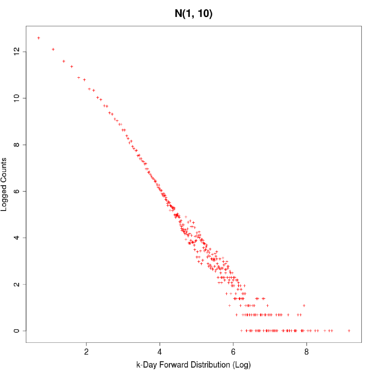
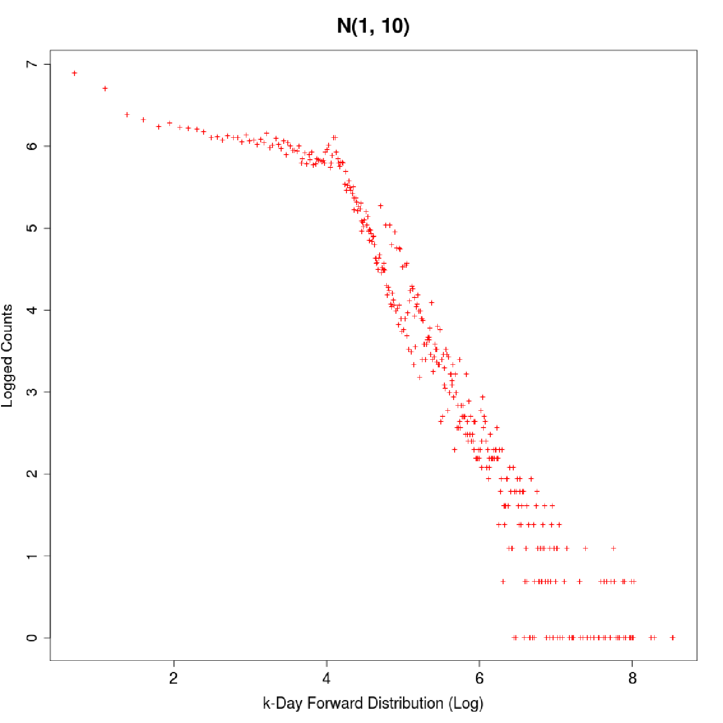
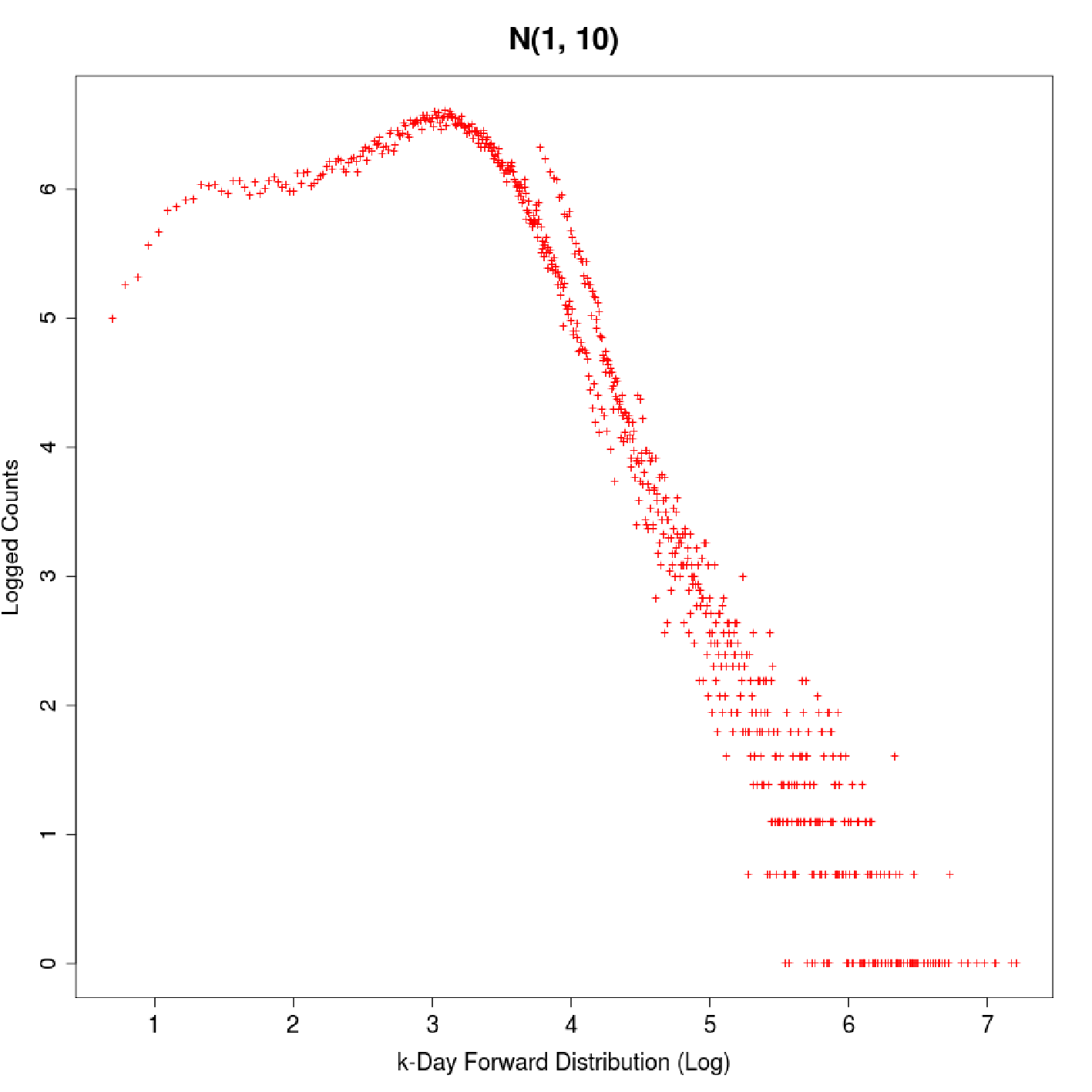
For a certain group , if we know today’s fame for each entity, what is the forward distribution of tomorrow’s fame? For example, for all entities currently with daily references in range (0,20), how their tomorrow’s frequencies are distributed? More generally, we denote and are the lower and upper bounds of historical frequencies/fame. If current day’s fame (with fame window size ) is in range , how tomorrow’s fame (with fame window size )is distributed? Here we can denote the fame as . In addition, we define that notion is the probability distribution of that frequency/fame is greater than some certain level . That is, the distribution is . Figure 11 shows that both the histogram plot of and the distribution have power-law tails, in spite of their different historical/future fame window sizes. However, the histogram plots 11(b),11(c), and 11(d) are somewhat truncated into two parts by certain truncation points. The truncation points are some values between and . If , the truncation value is exactly , just as the truncation point shown in Figure 11(c), with a value of .
Now Using a subset of our news database as the training data, we will apply this model to estimate the probabilities that some trivial entities become very famous. The results are shown in Table 4. Here both the historical fame window size and the future fame window size is set to 1 day. This table shows that some unknown entities with little fame (historical references 0200) became famous (future references ). Actually, Table 2 tells us that a reference of 3000 means a similar fame with Chicago. We divide entities into four categories according to their historical fame, (0-20), (20-50), (50-100), and (100-200) respectively, and then we train the data to get the slopes and y-intercepts to build four power-law models. We compare the entity counts and probabilities to become famous between real news data and our power-law models, and find they are very close. For example, while and , we have
| (10) |
To make , we get and the estimated counts to become famous is .
The final question is that what kind of entities become famous. Table 5 lists some unknown entities (with daily reference 20) became famous (with daily reference 1000 for 5 continuous days). We can see many of them became famous because of death, and some of them were because of political events. This tells us the interesting fact that media tends to remember people accompanied with their death. Some non-people entities could also become famous, e.g., “Sichan" and “Haiti" became famous because of earthquakes.
6 Group-based Fame Forecasting
Now we consider the fame change of entities within a specific domain or group context. The fact that an entity becomes famous means its fame changes dramatically, which indicates its future fame is significantly higher than its historical fame. For entities in a group over a future time range , the degree of fame-change could be measured by ratio or shown as below:
- •
- •
Next period peak fame is a function of future time range and peak fame window size . In our analysis, we make as 1 year and as 5 days.
Figure 13 indicates that the distributions of both and have power-law tails, although the slopes in their Log-Log plots are not exactly the same for different groups. The fitted linear lines are also shown in these Log-Log plots. Based on the power-law models, we can compute the probability that some entity within the group becomes famous in a future time range . We have
| (11) |
That is . By fitting and with a linear model, could be calculated. Table 6 examines the accuracy of the power-law model, which indicates the theoretical result and the real news data match very well.
Table 7 gives some examples that entities have big values of or . Indeed we can use distribution either or to calculate probabilities that entities become famous, but we may get slight different results with these two ratios.
Groups Size Next_Year_Peak_Fame/Historical_Fame Next_Year_Ave_Fame/Historical_Fame Real Data Our Model Real Data Our Model T Cnts Prob Slope Cnts Prob T Cnts Prob Slope Cnts Prob Top Cities 50 5 16 0.080 -3.202 21 0.107 2 17 0.085 -4.779 13 0.064 7 7 0.035 -3.202 7 0.036 2.5 5 0.025 -4.779 4 0.022 10 2 0.010 -3.202 2 0.010 3 2 0.01 -4.779 2 0.009 Representatives 439 50 101 5.75E-02 -1.828 101 5.76E-02 5 60 3.41E-02 -2.296 55 3.13E-02 100 33 1.88E-02 -1.828 28 1.62E-02 10 11 6.26E-03 -2.296 11 6.37E-03 200 7 3.99E-03 -1.828 8 4.57E-03 20 2 1.14E-03 -2.296 2 1.29E-03 CS Profs 1911 50 11 1.44E-03 -1.734 19 2.60E-03 3 16 2.09E-03 -2.803 30 4.00E-03 100 3 3.92E-04 -1.734 5 7.82E-04 5 4 5.23E-04 -2.803 7 9.56E-04 200 0 0 -1.734 2 2.34E-04 7 2 2.61E-04 -2.803 3 3.72E-04
Entity Name Group P/H A/H Peak Freqs Why become famous On When New Orleans Cities 10.23 1.30 24917 Hurricane Katrina 09/02/2005 Memphis Cities 12.39 2.54 7763 the first team in NCAA to achieve 30 wins in a season 04/07/2008 Omaha Cities 8.55 3.11 2622 June 2008 tornado outbreak sequence 06/12/2008 Tulsa Cities 9.64 3.76 5563 ice storm in December 12/26/2007 Kirsten Gillibrand Represen 458.8 24.2 5324 elected to the Senator of New York 01/23/2009 Joe Wilson Represen 491.7 13.2 23323 shouted at Obama during 2009 Presidential address 09/09/2009 Sebastian Thrun CS Profs 74.3 3.1 1091 helps GM to make robot driven cars 01/07/2008 Amar Bose CS Profs 51.2 3.7 652 retired from MIT 11/26/2005
- •
Probability of making zero-fame people famous
Based on the power-law tail, we can estimate what’s the probability that some people with almost zero fame became famous, e.g., as famous as Tiger Woods. From Table 2, we know Tiger Woods’ peak fame is 20,000, and we notice the power-law model () for CS professors (let’s assume this model is generally applicable to any group of people) is
| (12) |
While , we can get . We know there are 300 million people in the United States. Therefore, there are roughly million = 24 persons that will have comparable peak fame with Tiger Woods in the next 1 year.
But how about to reach Tiger Woods’ average fame? We know the power-law model () for CS professors is
| (13) |
Because Woods’ average fame is around 1000, our calculation shows there is only 0.1 person who has no previous fame at all but can reach Tiger Woods’ average fame in the next year. Similarly, Steve Jobs’ average fame is around 100, and our model shows there are roughly 64 unknown persons can reach Steve’s average fame in the next year.
In all previous cases, we make as 1 year to train power-law models. But how about 10 years? That is, what is probability of an unknown person become famous in the next 10 years? Let’s suppose the distribution of or follows Formula 11 for future time range . Now we could deduce the distribution for a time range of :
So we argue that the probability just increases linearly with the increasing of time.
7 Conclusions
This paper studied new entity and group modeling and forecasting methodologies, including group fame distribution analysis, group fame probability analysis, and group fame evolution over time. We show some important news entity and group statistical patterns could be described by log-normal or power-law distributions. We also proposed a HMM-based news generation model, which has never been used in news modeling before. We show that HMM models are more capable of describing news generations than simple Log-Normal models. Based on these analysis, we answered some interesting news forecasting questions. For example, what is the probability that an entity become the most famous one among its group? And what is the likelihood that a trivial entity becomes incredibly important in the next time period? Our analysis shows these questions could be solved by fitting power-law tails and we validated the model with several interesting news groups in different domains. Our study provides very useful insights for the analysis of issues in finance, political science, or social science.
References
- [1] A.-L. Barabasi, A. laszlo Barabasi, R. Albert, and H. Jeong. Mean-field theory for scale-free random networks, 1999.
- [2] D. M. Blei, A. Y. Ng, and M. I. Jordan. Latent dirichlet allocation. Journal of Machine Learning Research, 3 (2003) 993-1022, 2003.
- [3] S. Deerwester, S. Dumais, G. Furnas, R. Harshman, T. Landauer, K. Lochbaum, and L. Streeter. Computer information retrieval using latent semantic structure. US Patent 4,839,853, June 1989.
- [4] M. Gotz, J. Leskovec, M. Mcglohon, and C. Faloutsos. Modeling blog dynamics. In International Conference on Weblogs and Social Media, May 2009.
- [5] V. Ha-Thuc, Y. Mejova, C. Harris, and P. Srinivasan. A taxonomy-based approach for modeling and tracking news events in the social web. Working paper, 2009.
- [6] T. Hofmann. Probabilistic latent semantic indexing. In Proceedings of the 15th Uncertainity in Artificial Intelligence, 1999.
- [7] A. C. Johnson and N. T. Thomopoulos. Use of the left-truncated normal distribution for improving achieved service levels. In Decision Sciences Institute 2002 Annual Meeting Proceedings, 2002.
- [8] N. F. Johnson1, M. Spagat, J. A. Restrepo, O. Becerra, J. Camilo, Bohorquez, N. Suarez, E. M. Restrepo, and R. Zarama. Universal patterns underlying ongoing wars and terrorism. Working Paper, 2006.
- [9] W. E. Leland, M. S. Taqqu, W. Willinger, and D. V. Wilson. On the self-similar nature of ethernet traffic (extended version). 2(1):1–15, 1994.
- [10] J. Leskovec, L. Backstrom, and J. Kleinberg. Meme-tracking and the dynamics of the news cycle. In Proceedings of the 15th ACM SIGKDD international conference on Knowledge discovery and data mining, 2009.
- [11] L. Lloyd, D. Kechagias, and S. Skiena. Lydia: A system for large-scale news analysis. In Proceedings of 12th String Processing and Information Retrieval (SPIRE 2005), volume LNCS 3772, pages 161–166, Buenos Aires, Argentina, 2005.
- [12] M. Mitzenmacher. A brief history of generative models for power law and lognormal distributions. Internet Mathematics, 1:226–251, 2001.
- [13] B. Pulse. http://blogpulse.com.
- [14] B. Scope. http://www.blogscope.net.
- [15] G. I. Search. http://www.google.com/insights/search.
- [16] B. H. J. Sjoberg, Mikael; Albrectsen. Truncated power laws: a tool for understanding aggregation patterns in animals? Ecology Letters, 3:90–94, 2000.
- [17] K. Sun. Explanation of log-normal distributions and power-law distributions in biology and social science. Working Paper, May 2004.
- [18] G. Trends. http://www.google.com/trends.
- [19] M. Wang, T. Madhyastha, N. H. Chan, S. Papadimitriou, and C. Faloutsos. Data mining meets performance evaluation: fast algorithms for modeling bursty traffic. In Data Engineering, 2002. Proceedings. 18th International Conference on.