-boson spectrum from a Discrete Scale Invariance
Abstract
We present the analysis of the -boson spectrum computed using a soft two-body potential the strength of which has been varied in order to cover an extended range of positive and negative values of the two-body scattering length close to the unitary limit. The spectrum shows a tree structure of two states, one shallow and one deep, attached to the ground-state of the system with one less particle. It is governed by an unique universal function, , already known in the case of three bosons. In the three-particle system the angle , determined by the ratio of the two- and three-body binding energies , characterizes the Discrete Scale Invariance of the system. Extending the definition of the angle to the -body system as , we study the -boson spectrum in terms of this variable. The analysis of the results, obtained for up to bosons, allows us to extract a general formula for the energy levels of the system close to the unitary limit. Interestingly, a linear dependence of the universal function as a function of is observed at fixed values of . We show that the finite-range nature of the calculations results in the range corrections that generate a shift of the linear relation between the scattering length and a particular form of the universal function. We also comment on the limits of applicability of the universal relations.
I Introduction.
Physical systems present universal behavior when specific details of the interaction between their constituents are suppressed in favor of a few control parameters which determine the dynamics. Well-known examples of this kind are critical phenomena in which the systems, that are very different at the microscopic level, show a set of equal critical exponents. Around the critical point the dynamics is governed by long range correlations and not by the details of the interaction between the constituents. When a universal class is identified all systems belonging to this class can be described equally well by a model in which this particular phenomenon is implemented. As an example we can mentioned the Ising model to study phase transitions.
Here we analyze a particular universal behavior of few-boson systems having a large two-body scattering length. In two-body systems, the universality is governed by one parameter, the scattering length . When is large and positive the two-body system has a shallow bound state with an energy of (shallow dimer) and, in addition, all the low-energy observables are governed by . The system has a continuous scale invariance which strongly constrain the form of the observables. This symmetry is broken in the -wave three-body sector. However, the three-body system still has a residual symmetry - the discrete scale invariance (DSI) - meaning that the physics is invariant under the rescaling , where the constant is usually written as , with being a universal number that characterizes a system of three-identical bosons (for a recent review see Ref. [1])
As has been shown by V. Efimov [2, 3], in the limit of large scattering length, (unitary limit), the three-boson spectrum consists of an infinite number of states that accumulate to zero with the ratio between the energies of two consecutive states being . This is known as the Efimov effect and its characteristics have been the subject of an intense investigation from both experimental [4, 5, 6, 7] and theoretical [8, 9, 10, 11, 12] point of view. In recent years the study of the Efimov effect has been extended to what is now called Efimov physics and refers to the physics of shallow states. In these states the particles stay mostly far apart from each other with the consequence that the dynamics is largely insensitive to the details of the interaction.
In the case of bound states, the three-boson spectrum in the limit of zero-range interaction in two-body subsystem (zero-range limit or scaling limit) can be expressed in the following parametric form
| (1) |
where is the wave number corresponding to the energy of the -level at the unitary limit, and is called the three-body parameter. The function is a universal function and its parametrization in the range is given in Ref. [1]. The second line of the above equation explicitly manifests DSI: the ratio remains constant at each value of the angle and is equal to . Another characteristic of the above equation is that the three-boson spectrum is controlled by the two-body scattering length and it is completely determined by the knowledge of the three-body parameter , which appears as a scale parameter. Many examples of how Eq.(1) is used can be found in the literature (see for example Refs. [1, 17]).
In the four-body case, it has been shown that two levels, and appear attached to each level [9, 10, 11, 12, 13, 14]. Moreover, at the unitary limit the ratios and are universal and their numerical values have been estimated using different approaches. In Ref. [15] it has been shown that universal ratios also exist at the universal limit in systems with bosons and these ratios were estimated by solving the corresponding Schrödinger equation with finite-range two-body potentials. In Ref. [16] the spectra and universality of small helium clusters up to have been studied in the plane, where and is the energy of a level. The two lowest levels with the energies of and , attached to the ground state of the system, with energy of , have been observed in the region of studied. Furthermore in Refs. [15, 16] the values of at which the -body cluster disappears into the -body continuum have been estimated.
In the present work we address the constraints imposed by the DSI in the spectrum of the -boson system with a general number of bosons . In addition we will answer the following questions. 1) Is the tree structure of two states, and , attached to the state and observed up to , valid for general values of ? 2) Are there any general relations for the ratios and ? We answer these question by analyzing the spectra of particles obtained from solution of the many-body Schrödinger equation with a soft finite-range two-body force.
The paper is organized as follows. In the next section the working equations determining the spectrum of the -boson system are given. The analysis of the numerical results is given in Section III, whereas the DSI for bosons is analyzed in Section IV. In section V the equations proposed in the previous sections are used to analyze selected experimental as well as theoretical results from the literature. In the last section the conclusions are given.
II The -boson system in the zero-range limit.
Our aim is to discuss an extension of Eq.(1), that describes the energy spectrum of the three-boson system close to the unitary limit in the zero-range limit, to . This extension is based on the detailed analysis of a four-boson system with a large two-body scattering length, reported first in Ref. [9] and then in Refs. [10, 11], and on an extended analysis of DSI in Ref. [18]. It has been found in Ref. [9] that the four-body system has two bound states, one of which is deeply bound and another one is shallow being very close to the threshold of disintegration into one boson and a trimer. Using a DSI argument, it has been conjectured that the two-level structure is tied to each three-body state. However, only the lowest two states, attached to the trimer bound state , are true bound states; the other ones appear as resonances since they are above the trimer-particle threshold. The study of this particular tree structure has been analyzed in Ref. [10] in which the notation was proposed to identify the energy of each four-body level. In this notation, indicates a three-body level and identifies the deep state while labels the shallow state. The fact that this structure of levels results from a DSI can be seen from the universal character of the ratio . A study of this ratio at the unitary limit has been done in Refs. [10, 11] with the conclusion that and . A more extended analysis of the DSI can be done studying these ratios along the plane at fixed values of the angle (see Ref. [18]). Moreover, a recent work [19] has shown that the universal function , that governs the three-boson dynamics, is also responsible for the -boson dynamics. All these findings suggest the following extension of Eq.(1) to
| (2) |
with the deep () or shallow () -body state attached to the -th Efimov trimer.
Eq. (2) has the remarkable property that the - boson spectrum is controlled by the two-body scattering length, by the universal function , and that it is completely determined by the knowledge of .
The are not true-independent parameters; they are fixed by the three-body scale . For instance, in Ref. [19] it has been shown that
| (3) |
This result has been obtained by observing that is a linear function of and using the universal ratio given in Ref. [11]. In the following we analyze the spectrum of -boson systems up to in order to extend this relation to and, in a more general perspective, to verify the validity of Eq. (2).
III Finite-range corrections
The spectrum of the three-boson system, obtained by solving the Schrödinger equation with soft two-body potentials close to the unitary limit, has been analyzed in Refs. [20, 21]. It has been shown that Eq.(1) has to be modified in order to take into account the finite-range character of those calculations. Based on the analysis of the energies of the three-body system obtained numerically, the following modified equation has been deduced
| (4) |
Despite some similarities, there are several important differences to the zero-range theory of Eq.(1).
(i) The parameters carry explicitly the index labeling the different tree branches since the ratio for two successive branches is in general slightly different from the scaling factor . In fact these ratios include finite-range corrections and their specific values can be extracted from the numerical solutions. The correspondence between Eq.(1) and Eq.(4) is made by identifying the scale parameter with one of the parameters . For example in Ref. [20] the three-helium atom case was studied as a reference system and has been identified with , the branch corresponding to the first excited state.
(ii) The quantity is replaced by , which is the dimer binding energy in the case of positive scattering length or, for negative values of , the two-body virtual-state energy. Also in the second line is replaced by the scattering length corresponding to finite-range two-body potential. The replacement of by introduces some range corrections as the value of moves away from the unitary limit. It should be noticed that the relation is exact in the case of zero-range two-body interactions.
(iii) The main modification in Eq.(4) is the introduction of the shift parameter . The origin of the shift has been discussed in Ref. [19] where it has been shown that it essentially appears from the first order expansion of the scaling-violating momentum , in terms of powers of , where is the interaction range. The parameter fixes the value of the logarithmic derivative of the wave function close to the origin and encodes the short-range physics [1]. In the zero-range model one can identify with the three-body parameter leading directly to Eq.(1). However, for finite-range potentials the relation does not hold anymore and we propose the finite-range correction
| (5) |
leading directly to Eq.(4), with (here we assume ). This can be proved by making use of Eqs.(187) and (193) from Ref. [1].
As a function of the finite-range-corrected scattering length , Eq.(4) is a two-parameter equation: the scale parameter and the finite-range parameter . As in the study of critical phenomena, can be interpreted as a material-dependent parameter, and as the analogue of the finite-scale correction (here finite-range correction). Their introduction allows the collapse of observables onto a single universal curve [22]. In fact, in Ref. [19], it has been shown that plotting in terms of makes the calculated points to collapse onto a universal curve.
The extension of Eq.(4) to general has been proposed in Ref. [19] where the spectrum of the -boson system, obtained by solving the Schrödinger equation with soft potentials close to the unitary limit, has been analyzed up to . The results of that work have shown that Eq.(2) has to be modified in order to take into account the finite-range character of those calculations. The following general form has been deduced
| (6) |
and applied to the lowest tree of the two-level structure which correspond to . The index identify the branch and the index takes the value . However, unlike in the zero-range theory, the parameters explicitly show the index labeling the different branches due to the finite-range corrections in .
It should be stressed that, for , the case is of particular interest since it describes bound states. In the next section, we analyze the branch extracting the values from the numerical solutions and showing that they have a linear dependence with with a slope slightly different to the one suggested by the zero-range theory. We will show that, as moves from the unitary limit toward lower positive values, the validity of Eq.(6) could be limited. The system becomes more compact losing its universal character. In the case of the validity of Eq.(6) is limited by the appearance of different thresholds as the positive values of decrease. For example in Ref. [23] it was shown that, in the case, a shallow tetramer decays at the atom-trimer threshold becoming an inelastic virtual state. In the present work we limit the discussion of Eq.(6), in the case of , to the case of bound states ( branch).
IV Analysis of -body solutions.
To study the validity of Eqs.(2) and (6) we follow Ref. [16] and describe the -boson system using a two-body gaussian (TBG) potential
| (7) |
We solve the -body Schrödinger equation with mass parameter K. Using and K the model reproduces the binding energy and the scattering length of two helium atoms described by a widely used He-He interactions, the LM2M2 potential [24] which has a van der Waals length a.u..
To solve the Schrödinger equation for bosons we use the Hyperspherical Harmonic (HH) method in the version proposed in Ref.[25]. This method reproduces the values given in Ref. [26] up to and here we extend the calculations up to . Increasing the grand angular quantum number we obtain converged results for the ground state and first excited state of the -boson systems. As discussed in Refs. [25, 27], convergence of the ground state energy is obtained with relatively low values of ; with values of an accuracy greater than 1% is obtained. In the case of the first excited state a similar accuracy would need a much higher value of , making the computation of this state very difficult. In the present work we use the results with to extrapolate the first excited energy with an accuracy of a few percent.
Varying the strength of the TBG potential (7) we explore the plane. For each value of the potential strength we determine and and then compute the energies of the ground and first excited states of the -body systems. For we compute and - the values that define the first two energy branches with and . For we compute the two-level structure of the branch. We denote these states as and , omitting the index from now on, and we analyze the two-level spectrum up to .
Using the first line of Eqs. (4) and (6) we determine the value of the angle from which we can compute the universal function
| (8) |
appearing on the r.h.s of the second line of these equations. The function has a linear dependence on for each value of and . In fact, the second line of Eq.(6) can be rewritten as
| (9) |
In the case of zero-range interaction and , and the linear relation results in , representing a straight line passing through the origin with the slope determined by the value of . In the case of finite-range interaction the linear dependence between and remains but the straight line does not go through the origin.
To make connection with previous analysis, we first present our results for the case. Their plot in the plane have been reported many times in the literature. Here we prefer to use the plane stressing the linear relation between and that follows from Eq. (9). The results are shown in Fig. 1 as circles ( branch) and squares ( branch). The dashed lines represent the best linear fit to the results which can be parametrized with a.u.-1, and a.u.-1, . The fit has proving that the behavior of the numerical results is in very good agreement with a linear dependence. Moreover, at the unitary limit the extracted values for coincide up to four figures (or better) to the calculated values. The DSI predicts in the zero-range limit that while from our results we obtain a slightly different value, . This change originates due to the finite-range character of the two-body interaction.
The upper panel of Fig. 1 shows all calculated values plotted within a very extended range of . The lower panel displays a zoom around the thresholds , at which the trimer levels disappear into the three-body continuum (for a more precise value see Ref. [28]), and , at which the trimer disappears on the particle-dimer continuum (the thresholds are shown by thick horizontal lines). Close to the threshold at -1.56 we observe a strong linear trend in the behavior as a function of . This allows us to extract with a great confidence the (negative) values of the scattering length and at which the trimer ground state and first excited disappear into the three-atom continuum. Using the values of and from the linear fit and transforming to , we obtain a.u. and a.u. which are in close agreement with the estimates given in Ref. [16].
The threshold at 0.071 indicates the point at which the bound state disappears in the atom-dimer continuum. We cannot reach it by lowering the scattering length because as the three-body states become more bound leaving the Efimov window. For the case of the excited state this is less obvious but in the proximity to the atom-dimer threshold our results lie on a line parallel to (and slightly above) the line without crossing it. This has been also clearly seen in Ref. [16] where the first excited state for three Helium atoms has been shown not to cross the atom-dimer threshold but move almost parallel to it from below (see also Ref. [29]).

The analysis of the Efimov trimers in the plane has shown that they can be described by straight lines defined by parameters , and . Next, we study the results for in the same plane. These results are presented by circles in Fig. 2 which, as in the case, can be fitted by straight lines shown as solid lines in this figure. Panels (a) and (b) show the results for the ground state () and the first excited state () respectively. Panels (c) and (d) zoom the area around the threshold (shown as a thick line). In the case of very detailed calculations has been done close to this threshold.
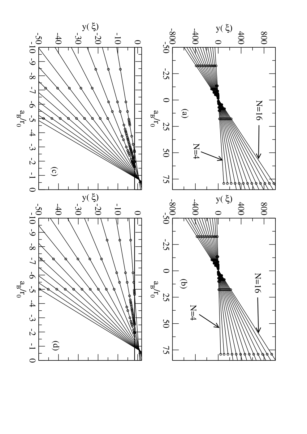
A remarkable characteristic of Fig. 2 is that the straight lines cross each other almost in one single point the position of which is slightly different for the ground and excited states. To study further this fact we extract the values of from the slopes of the straight lines. They coincide up to four significant figures with the values calculated at the unitary limit given by K. The results are given in Fig. 3 where we show: (a) the values of (circles) and (squares) as a function of and (b) the values of (circles) and (squares). The and form two almost parallel lines whereas and collapse in one line as increases. However, both and explicitly show a linear dependence with , which is illustrated in Fig. 4 where the best linear fits to the data are shown by the solid lines and the circles (squares) corresponds to (). Using this linear relation we extract the coordinates of the point at which the straight lines corresponding to the ground states, , and excited state, , cross each other. Defining , we obtain the relation between and :
| (10) |
From the analysis of Fig. 4 we get a.u. and for the ground states and a.u. and for the excited states. A consequence of the different location of these two points is that the line corresponding to the shallow state can cross the line of the ground state resulting in unbound excited state. This is shown in Fig. 5 where one can see that starting with the excited state is not bound anymore at the threshold.

Eq. (10) can be further simplified taking into account the linear relation between and . In fact, as has been inferred in Ref. [19], and from the analysis of Fig. 3, the relation can take the following form,
| (11) |
where we have used two points, corresponding to and to construct the line. However other choices to describe the straight line produces similar results. With the above relation, a global description of the th level of the -boson spectrum can be achieved with just four parameters.
The main result of this analysis is the following. In order to describe the th energy level of the -boson system, using short range interactions, two parameters are needed, and . This description is particularly accurate near the unitary limit. It deteriorates at positive values of as where the strength of the potential increases making the -body ground states deeper. In addition, as increases the finite character of the interaction allows new excited states to appear and the tree structure is lost. It was shown in Ref. [30] that starting with a second excited state appears at the unitary limit. However, the two-parameter description remains acceptable (of the order of a few percent or better) as the system approaches the -body continuum (negative values), which corresponds to the best realization of shallow states, well described by the present formalism. Approaching the threshold on the axis all the excited states disappear for , as has been discussed before. It should be noticed that in the case of a zero-range interaction there is only one parameter,, because , and, as the crossing point is the origin for the two -levels, the tree structure should remain valid with increasing .
In the case of finite-range interactions, using the relation given by Eq.(11), a global fit of the th level is possible for general values of with only four parameters: two values and the coordinates of the crossing point. However, this description is not as precise as the previous one and could introduce some errors. In the case of a zero-range interaction a global fit is possible with two parameters (two values of ) and, in this case the description should be exact. This is further analyzed in the next section.


V The DSI as a function of .
The DSI in the system can be seen from the constant values of the ratio between two different branches at fixed values of the angle . This property, in the zero-range theory, is encoded in Eq.(1) from which it is easy to see that, when is constant, then . Particular cases are the unitary limit corresponding to and the threshold at which the cluster disappear in the three-atom continuum corresponding to . However that property holds in all the range .
The extension of the zero-range theory to general is given in Eq.(2). This equation explicitly states the following property for the ratio between two different branches with general values of at fixed values of
| (12) |
Unlike in the case, no analytical expression for exists. It can be only determined from numerical analysis such as the one carried out in Ref. [11] for . However, we can show that depends linearly on by using Eq.(11) twice, for and . This results in formula (see also Ref. [19])
| (13) |
which in the zero-range limit reduces to when from Ref. [11] is used. Our numerical results using the TBG potential gives , showing some range corrections but not far from the zero-range limit. The square of Eq.(13) gives a quadratic dependence on of the -boson ground state energy expressed in terms of the three-boson ground state energy. A quadratic relation in terms of has been also obtained in Ref. [31].
Our results can be used to study different ratios that might display universal character. In Fig. 6 we show the ratios between ground states (circles), between the shallow state of the system and the ground state of the -body system, (triangles), and the ratio between the shallow states, (squares). At large the ratio tends to one suggesting that
| (14) |
This relation is a consequence of the almost constant behavior of the ratio (see Fig. 6) that allows Eq.(13) to be extended to shallow excited states of the tree structure for
| (15) |
which in the zero-range theory reduces to . The third general ratio can be obtained by observing that have a constant behavior. For the universal ratio of 1.002 can be used, which has been calculated in Ref. [11] in the zero-range theory making a detailed numerical analysis of the solution of the Faddeev-Yakubovsky equations (for comparison, our numerical results obtained with TBG potential give a value around ). This analysis complete the determination of the ratios given in Eq.(12).
Finally, Eq.(2) can be used to determine the relation between and at different thresholds at which the -body cluster disappears in the -body continuum. Using the notation for the corresponding value of , in the zero-range limit we have
| (16) |
This equation is an extension of the already known relation obtained in the zero-range case. In the case of finite-range interactions we use the working equation Eq.(6) and verify that the following modification of Eq.(16) is valid:
| (17) |
Here , with being the value at the threshold determined either from direct calculations or from a global linear fit. We evaluate using the calculated values for and . The results are given in Fig. 7 for both and . One can see that in both cases the quantity is close to the expected values of -2.33 () and -2.45 (). For is better represented by a constant supporting the global fit. For the quantity deviates from a constant within 10% (given by the shadowed area) since excited states’ binding energies have not completely converged. In particular the global fit for the excited states suffers from the fact that close to the threshold they are not bound any more for . We have to mention here that in Ref. [15] a different parametrization of exists that involves four parameters. Such a parametrization does not show universality.
In the case of positive values of , thresholds appear when the -body systems disappears into the continuum formed by the different clusterization of the -boson system. The first threshold appears at the -boson energy and it is formed by a cluster of bosons and one boson staying far apart. Other thresholds are formed by dimers (for even values of ) or by dimers plus a particle (for odd values of ). In the case of a detailed study of the behavior across the dimer-dimer and trimer-atom thresholds has been done in Ref. [23]. With increasing number of bosons the structure of the thresholds become more and more complicate. As discussed in the case, the validity of Eq.(2) for each system is limited by values of between and the appearance of the first threshold. An study of the behavior of the -boson system across these thresholds is at present underway.


VI Analysis of the results in different systems
Most of the studies of -boson systems with large two-body scattering lengths have been done either experimentally (real systems) or solving the Schrödinger equation using potential models for two-boson interaction. For example, here we have used a TBG potential, however, many other calculations with different model or realistic potentials can be found in the literature. In all these cases the deviations from the prediction of zero-range theory due to finite-range nature of two-body interactions cannot be ignored. The working equations, Eqs.(4) and (6), proposed here can be used to analyze results obtained elsewhere. In particular, the second line of these equations can be used to study the linear dependence between and (see Eq.(9)).
As a first example we analyze the binding energies of the system of three 7Li bosons measured in Ref. [32] for different values of the 7Li-7Li scattering length. From the values of the two- and three-body binding energies given in that reference we compute , the angle and the universal function . According to Eq.(9) the values of should depend linearly on . The results plotted in Fig. 8 do show the expected linear behavior thus providing a further confirmation of the finite-range theory given by Eq.(6). From the analysis of the straight line we extract the values and (see also Ref. [19]).
As a second example we analyze the results for boson clusters obtained at the unitary limit by J. von Stecher in Ref. [15] using gaussian potential models and including three-body forces. Empirically the results for in the region were parametrized in Ref. [15] as , where . In addition, the empirical relation has been deduced from the numerical result and the ratios have been calculated up to . The results from Ref. [15] cannot be plotted in the plane because the explicit values of and were not given. Instead we can plot them in the plane. The essential characteristics of this plot, given in the upper panel of Fig.9, remain the same with the slope, given by the ratio , and the shift related by the linear equation Eq.(10). The results lie on straight lines, as predicted by the finite-range theory proposed here. Moreover, the straight lines seem to cross each other in one single point and, accordingly can be described using a global fit with . This shift is negative and, in absolute value, it is slightly smaller than the value obtained here for in the global fit. In the lower panel of the figure the ratios are given as a function of . The diamonds are the results from Ref. [15]. At they follow a linear behavior presented by a dotted line fitted over this region. They lie below the universal line shown by the dashed line. On the other hand, our results, fitted by a solid line, are above the line of universality. The difference between our calculations and those from Ref. [15] is due to the absence of the repulsive three-body force in our case. With a two-body finite-range (gaussian) force only, the -boson clusters are more bound than in the zero-range case. Including three-body repulsive force reduces the strength of the linear dependence between and and eventually can reproduce the universal slope of 1.147. The particular three-body force, selected in Ref. [15] produces a ratio slightly lower than the universal one and, therefore, the slope of the straight dotted line in the bottom panel of Fig. 9 is smaller, which corresponds to less bound clusters. The calculations of Ref. [15] deviate from the linear behavior (dotted lines) for and practically follow the square root law. This is discussed below.
The lower panel of Fig.9 also presents the results for -boson clusters of polarized tritium obtained in Ref. [33] from a theoretical study within Diffusion Monte Carlo (DMC) method. In that work, the strength of the interaction has been varied to explore a wide range of the plane. The analysis of their results in the in the plane revealed that they lie on straight lines as predicted by the finite-range theory. Here we show the linear dependence of the energy wave numbers on at the unitary limit. This is illustrated by the squares whereas the dotted-dashed line represents a linear fit to the data.
Finally we analyze two calculations from literature performed for the ground state helium clusters with different numbers of using hard-core He-He potentials. From the published values of , it is possible to determine the angle and, from it, the values of the universal function . From the previous discussion we expect a linear relation between and , which means a quadratic dependence between and the ground state energy. To perform this analysis we use the results from by M. Lewerenz [34] and by Pandharipande et al. [35]. In the former, the ground states up to 10 atoms have been obtained within DMC with the TTY potential [36] as the He-He interaction. In the latter, the GFMC method has been used with the HFDHE2 interaction of Aziz et al. [37]. The extracted from these results are shown in Fig.10 where the black circles and stars correspond to the DMC calculations with TTY and the GFMC calculations with HFDHE2, respectively. We compare the hard-core results with those obtained with the soft-core TBG potentials in the present work, shown by squares. In addition, we show by triangles the results from Ref. [26] obtained with the TBG potential plus a hyperradial three-body force (H3B) the of which strength is fitted to reproduce the trimer energy given by the LM2M2 potential. It should be noticed that the TTY and the LM2M2 interactions produces very close results [39] for the helium dimer and trimer and, therefore, the results of the TBG+H3B interaction are almost on top of the results of the TTY potential. This support the equivalence between the soft and hard-core potentials for this kind of states, discussed for example in Ref. [38].
All above analyses show that the finite-range-corrected universality relations proposed in the present work can be used to analyze different types of measurements and theoretical descriptions of shallow states in bosonic systems. However, we notice that the results obtained with HFDHE2 and plotted in Fig.10 do not follow any more the linear behavior around . They tend to follow a square root behavior since at the ratio is almost constant indicating the well known linear dependence of the energy ground state with . It is interesting to notice that this analysis shows the transition between the quadratic and linear behavior of the ground state energy with . In the quadratic regime the bosons are well apart, the details of the interaction are not important and the system shows the universal behavior described by Eq.(6). As the number of bosons increases the system becomes more compact loosing the universal behavior. The strong short-range repulsion prevents the collapse of the system and is responsible for the linear regime. This explanation clarifies the behavior of the results from Ref. [15] for . In this case a very long-range repulsive three-body force has been included making the transition to the linear regime already at low values of . The observed transition from the quadratic to linear behavior for the case of realistic interaction with a (positive) large two-body scattering lengths is very interesting and in future should undergo a deeper analysis.


VII Conclusions
In the present work we have discussed DSI in shallow states of -boson systems. First of all, we have proposed an extension of universal relation, known from three-body zero-range theory, to using the results of Refs. [9, 10, 11, 16]. This is summarized in Eq.(2) which shows explicitly DSI and the two-level -body structure attached to each level of the three-boson system. Then we have extended Eq.(2) to include corrections due to the finite-range nature of the two-body interactions. These corrections are encoded in the shift which we introduce into Eq.(6) following Ref. [19]. At the origin of the extension of the universal equations to general is our finding that the universal function in the r.h.s. of Eq. (6) that governs the three-boson dynamics is the same as the one that governs the -boson dynamics. Such a conclusion has been made by analyzing the solutions of the Schrödinger equations obtained in Refs. [16, 19, 20, 21] with various model potentials. To our knowledge this remarkable fact was not anticipated before.
The second striking property of the universal equations (6) is the linear relation between , a particular form of the universal function, and (or in the zero-range theory). In the zero-range limit the straight lines go through the origin and, accordingly, the theory has only one parameter: the slope. In the case of finite-range interactions the linear relation between and still holds but the straight lines do not go through the origin and, therefore, the theory has two parameters: the slope and the distance along the axis to the origin given by the shift . This linear behavior follows from the linear dependence of the scale parameter and the finite-size scale parameter on . This property allows us to recover the universal -body relations in the zero-range limit.
We have checked if results available in the literature exhibit universal behavior given by Eq. (6). We have plotted in the plane the experimental data on the energies of the 7Li trimers, measured in Ref. [32] and proved that they show linear behavior. From the linear plot we extracted the values of and . At the unitary limit, we obtain , which can be checked either experimentally or theoretically. Furthermore, we have analyzed -body energies calculated in Refs. [15, 33] where a particular parametrization have been proposed. However, we have shown that in both cases the linear behavior in the plane persists thus restricting the number of parameters, needed to describe these systems, to two for each . Moreover those results show the expected linear dependence of the energy wave number on at the unitary limit. All these findings support both the zero-range and finite-range universal relations proposed here.
A further analysis shows that universal relations persist only for attractive two-body potentials. In real systems, a strong repulsion between atoms an short distances exists, which for fixed and (positive) finite values of leads to transition to the square root behavior of energy wave number with . For particular case of Ref. [35] this occurs around . At larger the wave numbers cannot be described by the zero-range theory which predicts a quadratic behavior of the ground state energy with . In this respect it would be interesting to study the boson clusters which have negative values of the two-body scattering length. In this case the shallow states are better realized and the transition between the quadratic and linear regime should occur at larger values on . In fact the results of Ref. [33] at the unitary limit show the transition at bigger values of than the results of Ref. [35] obtained at positive values of . We hope that these findings will stimulate new experimental and theoretical studies of -body shallow states.
References
- [1] E. Braaten and H. Hammer, Phys. Rep. 428, 259 (2006)
- [2] V. Efimov, Phys. Lett. B 33, 563 (1970)
- [3] V. Efimov, Sov.J.Nucl.Phys. 12, 589 (1971) [Yad.Fiz. 12, 1080 (1970)]
- [4] F. Ferlaino, and R. Grimm, Physics 3, 9 (2010)
- [5] M. Zaccanti et al., Nat. Phys. 5, 586 (2009); S. Roy et al., Phys. Rev Lett. 111, 053202 (2013)
- [6] F. Ferlaino et al., Few-Body Syst. 51, 113 (2011)
- [7] M. Berninger et al., Phys. Rev. Lett. 107, 120401 (2011)
- [8] L. Platter, H. W. Hammer and Ulf-G. Meissner, Phys. Rev. A 70, 052101 (2004)
- [9] H.-W. Hammer and L. Platter, Eur. Phys. J. A 32, 113 (2007)
- [10] J. von Stecher, J.P. D’Incao, and C.H. Greene, Nat. Phys. 5, 417 (2009)
- [11] A. Deltuva, R. Lazauskas and L. Platter, Few-Body Syst. 51, 235 (2011)
- [12] T. Frederico, L. Tomio, A. Delfino, M.R. Hadizadeh and M.T. Yamashita, Few-Body Syst. 51, 87 (2011)
- [13] L. Platter, Few-Body Syst. 43, 155 (2008)
- [14] M.R. Hadizadeh, M.T. amashita, L. Tomio, A. Delfino and T. Frederico, Phys. Rev. Lett. 107, 135304 (2011)
- [15] J. von Stecher, J. Phys. B: At. Mol. Opt. Phys. 43, 101002 (2010)
- [16] M. Gattobigio, A. Kievsky, A., and M. Viviani, Phys. Rev. A 86, 042513 (2012)
- [17] H.-W. Hammer and L. Platter, Ann. Rev. Nucl. Part. Sci. 60,207 (2010)
- [18] M. Gattobigio, A. Kievsky and M. Viviani, Few-Body Syst. 54, 1547 (2013)
- [19] M. Gattobigio and A. Kievsky, PRL submitted
- [20] A. Kievsky and M. Gattobigio, Phys. Rev. A 87, 052719 (2013)
- [21] E. Garrido, M. Gattobigio, and A. Kievsky, Phys. Rev. A 88, 032701 (2013)
- [22] H.E. Stanley, Rev. Mod. Phys. 71, S358 (1999)
- [23] A. Deltuva, Few-Body Syst. 54, 569 (2013)
- [24] R.A. Aziz, and M.J. Slaman, J. Chem. Phys. 94, 8047 (1991)
- [25] N.K. Timofeyuk, Phys. Rev. C 78, 054314 (2008)
- [26] M. Gattobigio, A. Kievsky, A., and M. Viviani, Phys. Rev. A 84, 052503 (2011)
- [27] N.K. Timofeyuk, Phys. Rev. A 86, 032507 (2012)
- [28] A. Gogolin, Ch. Mora, and R. Egger, Phys. Rev. Lett. 100, 140404 (2008)
- [29] S. Endo, P. Naidon, M. Ueda, Phys. Rev A 86, 062703 (2012)
- [30] A. Kievsky, M. Gattobigio and N.K. Timofeyuk, Few-Body Syst., in press
- [31] A. M. Nicholson, Phys. Rev. Lett. 109, 073003 (2012)
- [32] N. Gross et al., Comptes Rendus Physique 12, 4 (2011)
- [33] G.J. Hanna and D. Blume, Phys. Rev. A 74, 063604 (2006)
- [34] M. Lewerenz, J. Chem. Phys. 106, 4596 (1997)
- [35] V.R. Pandharipande, J.G. Zabolizky, S.C. Pieper, R.B. Wiringa, and U. Helmbrecht, Phys. Rev. Lett. 50, 1676 (1983)
- [36] K.T. Tang, J.P. Toennies and C.L. Yiu, Phys. Rev. Lett. 74, 1546 (1995)
- [37] R.A. Aziz, V.P.S. Nain, J.S. Carley, W.L. Taylor, and G.T. McConville, J. Chem. Phys. 70, 4330 (1979)
- [38] A. Kievsky, E. Garrido, C. Romero-Redondo and P. Barletta, Few-Body Syst. 51, 259 (2011)
- [39] P. Barletta and A. Kievsky, Phys. Rev. A 64, 042514 (2001)