On the rotation class of knotted Legendrian tori in $\mathbb{R}^{5}$Thanks: S. Baldridge was partially supported by NSF Grant DMS-0748636.

Compared to Legendrian knots in ${\mathbb{R}}^{3}$, little is known about knotted Legendrian submanifolds $L^{n}$ embedded in $\mathbb{R}^{2n+1}$. One reason is that in higher dimensions there are no standard representations of embedded Legendrian submanifolds that enable one to study with the same facility as front projections or Lagrangian projections of Legendrian knots in ${\mathbb{R}}^{3}$. For example, one may easily compute the classical invariants of Thurston-Bennequin and rotation numbers by looking at the front projection of a knot in $\mathbb{R}^{3}$. Moreover, the classical invariants are quite effective at distinguishing many knots up to Legendrian isotopy: torus knots, for example have been shown to be classified by their classical invariants (cf. [10]).

While the Thurston-Bennequin number may be generalized to higher dimensions, it is not always as useful as it is for knots in dimension $3$. In the case we study in this paper, knotted Legendrian tori $L\in\mathbb{R}^{5}$, the Thurston-Bennequin invariant is well defined (cf. [25]), but uninteresting since it is always equal to zero. In fact, the Thurston-Bennequin number in ${\mathbb{R}}^{2n+1}$ equals $\frac{1}{2}\chi(L)$ when $n$ is even. Furthermore, while topological knot type provides an additional invariant for Legendrian knots in ${\mathbb{R}}^{3}$, all knotted Legendrian surfaces in ${\mathbb{R}}^{5}$ are topologically equivalent provided they are of the same genus.

The rotation class is harder to generalize to higher dimensions. Unlike the Thurston-Bennequin number, which may be defined in terms of a linking number, the rotation number requires the computation of the homotopy class of a map from $L$ to the space of Lagrangians of ${\mathbb{R}}^{4}$ with symplectic structure induced by the contact form on ${\mathbb{R}}^{5}$. Since writing down this map is non-trivial this invariant is more difficult to compute in higher dimensions.

Lagrangian hypercube diagrams overcome the difficulties involved in studying knotted Legendrian tori in ${\mathbb{R}}^{5}$, by providing a way to construct explicit embeddings of Legendrian tori. Using the explicit map defined by a Lagrangian hypercube diagram we demonstrate that the rotation class may be calculated combinatorially as follows:

Recall that the Maslov index, as defined in [23] and [9], may be viewed as a map $\mu:H_{1}(L)\rightarrow{\mathbb{Z}}$.

The Maslov number of the torus $L$ is the smallest positive number that is the Maslov index of some nontrivial loop (cf. [9]). Thus Corollary 2 enables us to compute the Maslov number of $L$ as follows:

In [9], Ekholm, Etnyre, and Sullivan compute the classical invariants for Legendrian tori obtained by front-spinning, showing that, in particular, the rotation class of the surface so obtained, is determined by the rotation number of the front projection used in the construction. Thus, their construction leads to tori with rotation class of the form $(0,r)$. Not only are we able to construct Legendrian tori in which both factors of the torus are knotted, but we show that Legendrian tori constructed from hypercube diagrams realize every possible pair of integers under the isomorphism defined by $H\Gamma$. In particular, we get examples where the rotation class is $(0,r)$ in the following theorem by taking one of the knots to be a trivial knot with rotation number zero:

Theorem 4 is a statement about the existence of Lagrangian hypercube diagrams. The methods used in the proof to find Lagrangian hypercube diagrams lead in general to excessively large diagrams. In practice, however, Lagrangian hypercube diagrams are easy to build by hand. Knot theory benefited greatly because of the development of nice representations for the knots: braids, knot projections, grid diagrams, etc. Theorem 1 and 4 together can be viewed as our attempt to create similar useful representations of Legendrian tori in $\mathbb{R}^{5}$. In fact, computers can be used to easily generate and compute examples (see Theorem 8.4).

This paper stands alone as one of the first papers to explicitly compute classical Legendrian invariants for a large class of knotted Legendrian submanifolds in $\mathbb{R}^{2n+1}$ for $n\geq 2$ (cf. [9]). We see the potential for much more: this paper contains key elements in the computing the gradings and dimensions of the moduli spaces used in computing the differential in contact homology. Our future work will be on how to use the representations and the calculations in this paper to compute the contact homology algorithmically directly from Lagrangian hypercube diagrams.

In fact, we were particularly interested in studying the contact homology of embedded Legendrian tori in ${\mathbb{R}}^{5}$ (or $S^{5}$) because of their relationship to Special Lagrangian Cones used to study the String Theory Model in physics. Briefly, according to this model, our universe is a product of the standard Minkowsky space ${\mathbb{R}}^{4}$ with a Calabi-Yau $3$-fold $X$. Based upon physical grounds, the SYZ-conjecture of Strominger, Yau, and Zaslov (cf. [24]) expects that this Calabi-Yau 3-fold can be given a fibration by Special Lagrangian $3$-tori with possibly some singular fibers. To make this idea rigorous one needs control over the singularities, which are not understood well. One method used to study these singularities (cf. Haskins [12] and Joyce [13]) is to model them locally as special Lagrangian cones $C\subset{\mathbb{C}}^{3}$. A special Lagrangian cone can be characterized by its associated link $L=C\bigcap S^{5}$ (the link of the singularity), which turns out to be a minimal Legendrian surface. When the link type of $L$ is a sphere, then $C$ must be a special Lagrangian plane. The interesting tractable case appears to be when the link type is an embedded torus. Several authors (cf. Castro-Urbano [6], Haskins [12], Joyce [13]) have shown that there exist infinite families of nontrivial special Lagrangian cones arising from minimal embedded Legendrian tori. Some work is already being done by Aganagic, Ekholm, Ng, and Vafa [1] to understand the connection between contact homology and Lagrangian fillings. We see this paper as possibly laying groundwork for developing combinatorial tools to understand special Lagrangian cones through the lens of contact homology.

In Section 2 we present a definition for the rotation class in dimension $5$ and prove that it is characterized by a pair of integers. Section 3 discusses Lagrangian grid diagrams, which enable us to define a Lagrangian hypercube diagram in Section 4. In Section 5 we prove that a Lagrangian hypercube diagram represents an immersed Lagrangian torus in dimension 4. This torus is shown in Section 6 to lift to a Legendrian torus in ${\mathbb{R}}^{5}$ with the standard contact structure. We then prove Theorem 1 (Section 7) and close with a proof of Theorem 4 and further examples (Section 8).

In [9] the classical Legendrian invariants of Thurston-Bennequin number and rotation number are generalized for ${\mathbb{R}}^{2n+1}$. We recall the definition of rotation class for ${\mathbb{R}}^{5}$ here. Let $\mathbb{R}^{5}$ be parametrized using $wxyzt$-coordinates. Then $\alpha=dt-ydw-xdz$ is a contact $1$-form representing the standard contact structure on $\mathbb{R}^{5}$. The contact hyperplanes are given by:

Let $f:L\rightarrow({\mathbb{R}}^{5},\xi)$ be a Legendrian immersion. Then the image of $df_{x}:T_{x}L\rightarrow T_{f(x)}{\mathbb{R}}^{5}$ is a Lagrangian subspace of the contact hyperplane $\xi_{f(x)}$. Choose the complex structure $J:\xi_{(w,x,y,z,t)}\rightarrow\xi_{(w,x,y,z,t)}$ such that $J(\partial_{w}+y\partial_{t})=\partial_{y}$, $J(\partial_{y})=-(\partial_{w}+y\partial_{t})$, $J(\partial_{z}+x\partial_{t})=\partial_{x}$, and $J(\partial_{x})=-(\partial_{z}+x\partial_{t})$. Then the complexification $df_{\mathbb{C}}:TL\otimes{\mathbb{C}}\rightarrow\xi$ is a fiberwise bundle isomorphism. The homotopy class of $(f,df_{\mathbb{C}})$ is called the rotation class of $L$. Note that the Lagrangian projection $\pi_{t}:{\mathbb{R}}^{5}\rightarrow{\mathbb{C}}^{4}$ gives a complex isomorphism between $(\xi,J)$ and the trivial bundle with fiber ${\mathbb{C}}^{2}$. Composing $df_{\mathbb{C}}$ with $\pi_{t}$ we get a trivialization $TL\otimes{\mathbb{C}}\rightarrow{\mathbb{C}}^{2}$, which we identify with $df_{\mathbb{C}}$. Furthermore, we choose Hermitian metrics on $TL\otimes{\mathbb{C}}$ and ${\mathbb{C}}^{2}$ so that $df_{\mathbb{C}}$ is unitary. Thus $f$ gives rise to an element of $U(TL\otimes{\mathbb{C}},{\mathbb{C}}^{2})$. The group of continuous maps $C(L,U(2))$ acts freely and transitively on $U(TL\otimes{\mathbb{C}},{\mathbb{C}}^{2})$ and hence $\pi_{0}(U(TL\otimes{\mathbb{C}},{\mathbb{C}}^{2}))$ is in one to one correspondence with $[L,U(2)]$. From this point forward, we will consider $r(L)$ as an element $[L,U(2)]$.

In general, if $L$ is a genus $g$ Legendrian surface in ${\mathbb{R}}^{5}$, then the rotation class is an element of $[\Sigma_{g},U(2)]$. When $g=0$, $[S^{2},U(2)]\cong\pi_{2}(U(2))$, and hence, the rotation class is always trivial, and uninteresting (for spheres, neither classical invariant yields any useful information). However, when $g\geq 1$, the rotation class can be nontrivial. In fact,

The existence of the isomorphism in Theorem 2.1 is, by itself, not useful in general for calculations due to the fact that the isomorphism depends heavily upon the choice of loops on the torus used to define the map: a generic embedding $i:T^{2}\rightarrow\mathbb{R}^{5}$ does not have a preferred basis for homology (one can precompose with any element of $SL(2,\mathbb{Z})$ for example). However, Lagrangian hypercube diagrams do provide natural, albeit not canonical, choices for these loops as the torus is embedded in $\mathbb{R}^{5}$ (cf. $\tilde{\gamma}_{zx}$ and $\tilde{\gamma}_{wy}$ in Theorem 6.1). It is these choices together with Theorem 2.1 that allows us to write down our “preferred” calculations of rotation class and Maslov index for loops in the embedded Legendrian torus. The calculations are important to our future work in computing contact homology of knotted Legendrian tori algorithmically. While all of our calculations in computing the contact homology from a Lagrangian hypercube diagram will depend upon these choices, the contact homology calculation in the end will not.

Before moving on to the definition of a Lagrangian hypercube diagram, we begin with a discussion of Lagrangian grid diagrams.

Let $\mathbb{R}^{3}$ be given $wyt$-coordinates. Then $\alpha=dt-ydw$ is a contact $1$-form representing the standard contact structure on $\mathbb{R}^{3}$. The contact planes are given by:

A Legendrian knot in $({\mathbb{R}}^{3},\xi)$ is an embedding $L:S^{1}\rightarrow{\mathbb{R}}^{3}$ whose tangent vectors always lie in the contact planes determined by $\xi$. Let $\theta\mapsto(w(\theta),y(\theta),t(\theta))$ be a parametrization of $L$. There are two standard projections used to study Legendrian knots, the front projection:

and the Lagrangian projection:

In general, a given knot diagram will not represent the Lagrangian projection of a Legendrian knot. However, an immersion $\gamma:S^{1}\rightarrow{\mathbb{R}}^{2}:\theta\mapsto(w(\theta),y(\theta))$ will correspond to the Lagrangian projection of a Legendrian knot in $({\mathbb{R}}^{3},\xi)$ if the following hold:

We now translate 3.1 and 3.2 in the context of grid diagrams. Let $\hat{G}$ be a $wy$-oriented grid diagram (cf. [2]). Grid diagrams have been studied extensively in [8], [14], [15], [20], [22], and consists of an $n\times n$ grid together with a set of markings that, when connected by edges, represent a knot diagram. Typically one assigns the $y$-parallel segments in $\hat{G}$ to be the over-strands at any crossing. However, in the following definition we will ignore such crossing conditions, and think of $\hat{G}$ as an immersed $S^{1}$.

An immersed grid diagram $G$ may be thought of as a mapping $\gamma:S^{1}\rightarrow{\mathbb{R}}^{2}:\theta\mapsto(w(\theta),y(\theta))$. Since $w^{\prime}(\theta)$ is $0$ along any segment in $G$ parallel to the $y$-axis, and $y(\theta)$ is constant along any segment parallel to the $w$-axis, Condition 3.1 translates into

where $\{a_{i}\}$ is the collection of segments of $G$ parallel to the $w$-axis, $y_{i}$ is the $y$-coordinate of $a_{i}$, and $\sigma(a_{i})$ is $+1$ if $a_{i}$ is oriented left to right and $-1$ otherwise. Given a crossing in $G$ (i.e. given $\theta_{0}<\theta_{1}$ such that $\gamma(\theta_{0})=\gamma(\theta_{1})$), Condition 3.2 becomes:

where $\{c_{i}\}$ is the set of $w$-parallel segments in the loop beginning and ending at the given crossing and such that $\gamma(\theta)\neq\gamma(\theta_{0})$ for all $\theta\in(\theta_{0},\theta_{1})$. Condition 3.1 guarantees that choosing the other loop $(\theta_{1},\theta_{0})\in{\mathbb{R}}/{2\pi{\mathbb{Z}}}$ will give the same integral up to sign as the one chosen. Therefore any immersed grid diagram $G$ satisfying Conditions (1) and (2) lifts to a piecewise linear Legendrian knot in $({\mathbb{R}}^{3},\xi)$ as follows: choose some $\theta_{0}\in S^{1}$ and define the $t$-coordinate $t_{0}$ of $\gamma(\theta_{0})$ to be $0$. Then define

Condition 3.1 guarantees that in defining the $t$-coordinate this way, the lift will be a closed loop. Condition 3.2 guarantees that the vertical and horizontal segments at a crossing will have different $t$-coordinates.

Given a Lagrangian projection of a Legendrian knot $L$, one may compute the rotation number as follows. Use the vector field $w=\frac{\partial}{\partial y}$ to trivialize $\xi|_{L}$. Then the rotation number may be calculated to be the winding number of the tangent vector to $L$ with respect to this trivialization:

For a Lagrangian grid, this is simply a signed count of the corners of $G$. Let $B$ be the collection of corners in $G$. Then for a corner $b\in B$ let $\eta(b)$ be a function that assigns a value of $+1$ to any corner of type $W:{NE}$, $Y:{NW}$, $W:{SW}$, and $Y:{SE}$ (i.e. a counterclockwise oriented corner), and a value of $-1$ to any corner of type $W:{NW}$, $Y:{NE}$, $W:{SE}$, and $Y:{SW}$ (i.e. a clockwise oriented corner) following the same notation as in [22] and [21]. Figure 2 illustrates the types of corners. Thus we observe that:

The Legendrian knots produced using the above method will be piecewise linear, not smooth. However, we can produce smoothly embedded knots as follows. Choose $0<\epsilon<<1$. Delete an $\epsilon$ neighborhood of each vertex of $G$ and replace it with a smooth curve (cf. Figure 4). Such a smoothing may be accomplished so as to guarantee that the diagram is smooth at the boundary of the $\epsilon$ neighborhood as well. For example, the image of the map

allows one to replace a $W:{SE}$ corner with a smooth arc, but the resulting rounded corner will only be $C^{1}$ at the boundary of the $\epsilon$ neighborhood. Note that the smoothing may be done so that the resulting curve is symmetric about the line of slope $\pm 1$ through the vertex of the bend. Furthermore, given a choice of a smoothing at a corner such that the area enclosed by the smooth curve and the original bend is $A$, one may obtain a different smoothing so that the area enclosed is $rA$ where $r\in{\mathbb{R}}$ such that $0<r\leq 1$.

Note if $A_{i,j}=A$ for all $i,j$, the above sum evaluates to $4Ar(G)$. Thus, if the rotation number is $0$ then the same smoothing may be used for all vertices of $G$.

Proposition 3.5 and Corollary 3.6 show that a Lagrangian grid diagram corresponds to a smoothly embedded Legendrian knot that does not depend on the choice of epsilon used in the smoothing. Hence we may refer to the Legendrian knot corresponding to a Lagrangian grid diagram.

The Legendrian lift of the smoothed Lagrangian grid diagram is unique up to Legendrian isotopy (Proposition 3.5). By Corollary 3.6 we can do integer calculations directly from the Lagrangian grid diagram instead of the smooth $\gamma_{\epsilon}$ loop, without worrying about changing the crossing information of the lift of the Lagrangian grid diagram. In particular, there is a correspondence of horizontal edges with opposite orientation in each column that allows one to re-interpret the Lagrangian grid conditions as a signed area sum. That is:

In practice, the area calculation described in the previous example may be carried out by simply decomposing the grid into polygonal regions where the top-most horizontal edges are all oriented left (resp. right) and the bottom-most horizontal edges are all oriented right (resp. left). Then, the signed area of these polygonal regions will correspond to the integrals defined in Conditions 3.1 and 3.2. For convenience, in the proofs that follow, we will use this signed area calculation to compute the integrals defined in Conditions 3.1 and 3.2.

Before proving the theorem, we introduce some definitions and lemmas that we will use only for the proofs in this paper.

Let the $t$-coordinate of $\gamma(0)$ be $0$. Then define,

Thus the last condition of Definition 3.12 guarantees that an almost Lagrangian grid diagram gives rise to an embedded Legendrian arc. Since the endpoints of this arc project to the top right corner marking and differ only in their $t$-coordinates, an almost Lagrangian grid diagram still gives rise to a knot in ${\mathbb{R}}^{3}$ by attaching the endpoints by a segment parallel to the $t$-axis.

We now proceed with the proof of Theorem 3.11.

The definition of a Lagrangian hypercube diagram codifies a data structure that mimics that of hypercube diagrams, cube diagrams and grid diagrams. While the definition appears similar to that of $4$-dimensional hypercube diagrams as defined in [2], they are not equivalent. Let $n$ be a positive integer and let the hypercube $C=[0,n]\times[0,n]\times[0,n]\times[0,n]\subset\mathbb{R}^{4}$ be thought of as a $4$-dimensional Cartesian grid, i.e., a grid with integer valued vertices with axes $w$, $x$, $y$, and $z$. Orient $\mathbb{R}^{4}$ with the orientation $w\wedge x\wedge y\wedge z$.

A flat is any right rectangular $4$-dimensional prism with integer valued vertices in the hypercube such that there are two orthogonal edges at a vertex of length $n$ and the remaining two orthogonal edges are of length $1$. Name flats by the axes parallel to the two orthogonal edges of length $n$. For example, a $yz$-flat is a flat that has a face that is an $n\times n$ square that is parallel to the $yz$-plane.

Similarly, a cube is any right rectangular $4$-dimensional prism with integer vertices in the hypercube such that there are three orthogonal edges of length $n$ at a vertex with the remaining orthogonal edge of length $1$. Name cubes by the three edges of the cube of length $n$. See Figure 9 for examples.

A marking is a labeled point in $\mathbb{R}^{4}$ with half-integer coordinates. Mark unit hypercubes in the $4$-dimensional Cartesian grid with either a $W$, $X$, $Y$, or $Z$ such that the following marking conditions hold:

• •

  each cube has exactly one $W$, one $X$, one $Y$, and one $Z$ marking;
  

• •

  each cube has exactly two flats containing exactly 3 markings in each;
  

• •

  for each flat containing exactly 3 markings, the markings in that flat form a right angle such that each ray is parallel to a coordinate axis;
  

• •

  for each flat containing exactly 3 markings, the marking that is the vertex of the right angle is $W$ if and only if the flat is a $zw$-flat, $X$ if and only if the flat is a $wx$-flat, $Y$ if and only if the flat is a $xy$-flat, and $Z$ if and only if the flat is a $yz$-flat.

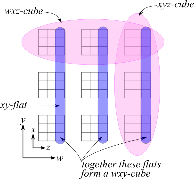
The 4th condition rules out the possibility of either $wy$-flats or a $zx$-flats with three markings. As with oriented grid diagrams and cube diagrams, we obtain an oriented link from the markings by connecting each $W$ marking to an $X$ marking by a segment parallel to the $w$-axis, each $X$ marking to a $W$ marking by a segment parallel to the $x$-axis, and so on.

Let $\pi_{xz},\pi_{wy}:{\mathbb{R}}^{4}\rightarrow{\mathbb{R}}^{2}$ be the natural projections. Define $G_{wy}:=\pi_{xz}(C)$ and $G_{zx}:=\pi_{wy}(C)$ which are immersed grid diagrams. Let $\{c_{i}\}$ be the crossings in $G_{zx}$, and $\{c_{i}^{\prime}\}$ be the crossings in $G_{wy}$. Then we say that the Lagrangian crossing conditions hold for the pair $G_{zx}$ and $G_{wy}$ if $|\Delta t(c_{i})|\neq|\Delta t(c_{i}^{\prime})|$ $\forall i,j$ where $\Delta t$ is the difference in the $t$-coordinates at each crossing determined by Equation 3.2.

A hypercube schematic (cf. Figure 10) conveniently displays the markings of a Lagrangian hypercube diagram so that the Lagrangian grid diagrams $G_{zx}$ and $G_{wy}$ may be read off of the diagrams directly. To see $G_{wy}$ treat each $n\times n$ $zx$-flat as a cell of $G_{wy}$ (i.e. consider the projection $\pi_{x}\circ\pi_{z}$). Each $zx$-flat containing a $W$ and $Z$ marking will project to a cell of $G_{wy}$ containing a $W$ marking and each $zx$-flat containing an $X$ and $Y$ marking will project to a cell of $G_{wy}$ containing a $Y$ marking. In Figure 10, the blue shading indicates the diagram associated to $G_{wy}$. To see $G_{zx}$ in the schematic, note that each pair of markings in a $zx$-flat on the schematic corresponds to an edge of the Lagrangian grid diagram $G_{zx}$. Placing these segments on a single $n\times n$ grid will produce a copy of $G_{zx}$.

To produce an immersed torus from the Lagrangian hypercube diagram, place a copy of the immersed grid $G_{zx}$ at each $zx$-flat on the schematic that contains a pair of markings (shown in red on Figure 10). Doing so produces a schematic with two copies of $G_{zx}$ with the same $y$-coordinates and two with the same $w$-coordinates. For each pair of copies sharing the same $w$-coordiantes, we may translate one parallel to the $w$-axis toward the other. Doing so traces out an immersed tube connecting these two copies of $G_{zx}$. Similarly, we may translate parallel to the $y$-axis to produce an immersed tube connecting two copies of $G_{zx}$ with the same $y$-coordinates. Since we are connecting copies of $G_{zx}$ in flats corresponding to the markings of $G_{wy}$, the tube will close to produce an immersed torus. Thus we obtain:

Since the torus is formed by the translation of $x$ and $z$-parallel segments to the $w$ and $y$ axes, we see that only $wx$, $wz$, $yz$, and $xy$ rectangles are used in the construction of the torus. Since $wy$ and $zx$ rectangles are never used in the construction of the torus, it is Lagrangian with respect to the symplectic form $dw\wedge dy+dz\wedge dx$. Furthermore, just as in the case of Lagrangian grid diagrams, we obtained a smooth embedding by carefully smoothing corners, we may obtain a smooth embedding of the torus in ${\mathbb{R}}^{5}$ by first smoothing $G_{zx}$ and $G_{wy}$ as in Lemma 3.5.

Furthermore, the torus has only two types of singularities: double point circles and intersections of double point circles. Each crossing of $G_{zx}$ generates a double point circle as shown by the yellow dots in Figure 10. Similarly each crossing of $G_{wy}$ generates a double point circle, which is visible in the schematic as the $zx$-flat where a $w$-parallel tube passes through a $y$-parallel tube. In Figure 10 this is shown by the yellow diagram. The green dot in Figure 10 corresponds to an intersection of two double point circles.

Let $i:T\rightarrow\mathbb{R}^{4}$ be the immersed torus obtained from a Lagrangian hypercube diagram as given by Theorem 5.1. Note that, $d\alpha|_{wxyz-hyperplane}=\omega=dw\wedge dy+dz\wedge dx$ is a symplectic form on $\mathbb{R}^{5}$. We will show that $H\Gamma$ represents the Lagrangian projection of a Legendrian surface in $\mathbb{R}^{5}$ with respect to the standard contact structure $\xi$.

In order to lift $i(T)$ we begin by choosing some point $p\in i(T)$ to have $t$ coordinate equal to some $t_{0}\in{\mathbb{R}}$. If we attempt to lift $i(T)$ to a Legendrian surface with respect to $\alpha$ we should choose to define the $t$-coordinate of $p^{\prime}\neq p$ to be:

where $\gamma$ is a path from $p$ to $p^{\prime}$. This integral will be independent of path precisely when the $1$-form $i^{*}(ydw+xdz)$ is $0$ on $H_{1}(T)$. Recall that $H_{1}(T)$ is generated by $\gamma_{zx}$ and $\gamma_{wy}$.

In order check for path-independence of the integral in Equation 6.1, we evaluate the following:

Since $G_{zx}$ and $G_{wy}$ are Lagrangian grid diagrams, these integrals will both evaluate to $0$ and we get a well-defined lift to a Legendrian torus in $\mathbb{R}^{5}$ using Equation 6.1. Furthermore, the Lagrangian crossing conditions guarantee that the lift will be embedded. Let $L$ be the lift of $i(T)$ obtained from Equation 6.1. Define $\pi_{t}:\mathbb{R}^{5}\rightarrow\mathbb{R}^{4}$ to be the projection $(w,x,y,z,t)\mapsto(w,x,y,z)$. Then $\pi_{t}(L)=i(T)$, i.e. the torus determined by $H\Gamma$ is the Lagrangian projection of the Legendrian torus $L$. Thus we obtain the following:

With the rotation class understood to be an element of $[T,U(2)]$ we see from Theorem 2.1 that the class may be identified with a pair of integers corresponding to the elements of $\pi_{1}(U(2))$ determined by a meridian and longitude of the torus. Before proving Theorem 1 we identify an explicit generator of $\pi_{1}(U(2))$. Recall that $U(2)$ parametrizes framed Lagrangians of $({\mathbb{R}}^{2},\omega)$. Identify the $yx$, $xy$, $yz$, and $zy$ planes with the following matrices:

Note that $U_{xy}$, $U_{xy}$, $U_{yz}$, and $U_{zy}$ correspond to unitary Lagrangian frames (cf. [18]):

Note that as maps from ${\mathbb{R}}^{2}\rightarrow{\mathbb{R}}^{4}$ these frames produce $xy$, $(-x)y$, $(-z)y$, and $zy$-planes respectively. Geometrically, this matches up with the fact that the Lagrangian planes along an $xz$-slice of the hypercube will be given by a positively or negatively oriented $\partial_{x}$ or $\partial_{z}$ vector paired with a positively oriented $\partial_{y}$-vector.

Choose $U_{xy}$ to be the basepoint. We define a loop $\gamma:[0,1]\rightarrow U(2)$ that begins at $U_{xy}$ and rotates through $U_{yz}$, $U_{yx}$ and $U_{zy}$. We will define $\gamma$ in $4$ pieces. First, define a map $\hat{\gamma}:[0,1]\rightarrow U(2)$ as follows:

Then, define $\gamma_{1}(t)=\hat{\gamma}(t)U_{xy}$, $\gamma_{2}(t)=\hat{\gamma}(t)U_{yz}$, $\gamma_{3}(t)=\hat{\gamma}(t)U_{yx}$, and $\gamma_{4}(t)=\hat{\gamma}(t)U_{zy}$. Finally, define $\gamma(t)=\gamma_{1}\star\gamma_{2}\star\gamma_{3}\star\gamma_{4}$. Thus $\gamma$ corresponds to a rotation of Lagrangian planes, beginning at an $xy$-plane, and rotating through $yz$, $yx$, and $zy$-planes.

The same argument will show that there is a generator for $\pi_{1}(U(2))$ given by acting on matrices $U_{xy}$, $\hat{U}_{yx}$, $U_{xw}$, and $U_{wx}$ on the left by:

Note that $U_{yx}\neq\hat{U}_{yx}$ as matrices in $U(2)$ but they give rise to the same Lagrangian planes, with the same orientation. While $U_{yx}$ corresponds to a unitary Lagrangian frame giving rise to the Lagrangian plane $\{-\partial_{x},\partial_{y}\}$, $\hat{U}_{yx}$ gives rise to the Lagrangian plane $\{\partial_{x},-\partial_{y}\}$.

References

- [1] M. Aganagic, T. Ekholm, L. Ng, C. Vafa. Topological Strings, D-Model, and Knot Contact Homology. arXiv:1304.5778 (2013).
- [2] S. Baldridge. Embedded and Lagrangian Tori in and Hypercube Homology. arXiv:1010.3742.
- [3] S. Baldridge, A. Lowrance. Cube diagrams and 3-dimensional Reidemeister-like Moves for Knots. Journal of Knot Theory and its Ramifications. DOI No: 10.1142/S0218216511009832.
- [4] S. Baldridge, B. McCarty. Small Examples of Cube Diagrams of Knots.Topology Proceedings. 36 (2010) pp. 213-228.
- [5] S. Baldridge, A. Lowrance. Cube Knot Calculator, http://cubeknots.googlecode.com.
- [6] I. Castro, F. Urbano. New examples of minimal Lagrangian tori in the complex projective plane. Manuscipta Math. 85 (1994) 265-281.
- [7] I. Castor, F. Urbano. On a minimal Lagrangian submanifold of foliated by spheres. Michigan Mathematical Journal. 46 (1999) 71-82.
- [8] P. Cromwell. Embedding knots and links in an open book. I. Basic properties. Topology Appl., 64 (1995), no. 1, pp. 37-58.
- [9] T. Ekholm, J. Etnyre, and M. Sullivan. Non-isotopic Legendrian submanifolds in . Journal of Differential Geometry. Volume 71, Number 1 (2005), 85-128.
- [10] J. B. Etnyre, K. Honda. Knots and Contact Geometry I: Torus knots and the Figure Eight Knot. Journal of Symplectic Geometry. Volume 1, Number 1, (2001), pp. 63-120.
- [11] J. B. Etnyre. Legendrian and Transversal Knots. In the Handbook of Knot Theory (Elsevier B. V., Amsterdam), (2005), 105-185.
- [12] M. Haskins. Special Lagrangian cones. American Journal of Mathematics. Volume 126, No. 4, August 2004, 845-871.
- [13] D. Joyce. Special Lagrangian -folds in with symmetries. Duke Mathematical Journal. Volume 115, No. 1 (1992).
- [14] C. Manolescu, P. Ozsvath, S. Sarkar. A combinatorial description of knot Floer homology. arXiv:math/0607691v2.
- [15] C. Manolescu, P. Ozsvath, Z. Szabo, D. Thurston. On combinatorial link Floer homology. arXiv:math/0610559v2.
- [16] B. McCarty. Cube number can detect chirality and Legendrian type of knots. Journal of Knot Theory and its Ramifications. DOI No: 10.1142/S0218216511009662.
- [17] B. McCarty. An infinite family of Legendrian torus knots distinguished by cube number. Topology and its Applications. DOI No: 10.1016/j.topol.2011.08.022.
- [18] D. McDuff, D. Salamon. Introduction to Symplectic Topology. Oxford University Press. 2nd Edition. (1999).
- [19] L. Ng. Computable Legendrian Invariants. Topology. Vol. 42, Issue 1, January 2003, pp. 55-82.
- [20] L. Ng. On arc index and maximal Thurston-Bennequin number. arXiv:math/0612356v3.
- [21] L. Ng, D. Thurston. Grid Diagrams, Braids, and Contact Geometry. Proceedings of the 13th Goköva Geometric-Topology Conference. pp. 1-17. (2008).
- [22] P. Ozvath, Z. Szabo, D. Thurston. Legendrian knots, transverse knots and combinatorial Floer homology. arXiv:math/0611841v2.
- [23] J. Robbin, D. Salamon. The Maslov Index for Paths. Topology 32 (1993), no. 4, 827 - 844.
- [24] A. Strominger, S.T. Yau, and E. Zaslow. Mirror symmetry and T-duality. Nuclear Physics B. 479 (1996) 243-259.
- [25] S. Tabachnikov. An invariant of a submanifold that is transversal to a distribution, (Russian). Uspekhi Mat. Nauk. Volume 43, Number 3(261), (1988), 193�194. Translation in Russian Math. Surveys 43 (1988), no. 3, 225�226.
- [26] G. W. Whitehead. On mappings into group-like spaces. Commentarii Mathematici Helvetici. Volume 28, Number 1, 320-328, 1954.